Realistic Representation of Grain Shapes in CFD–DEM Simulations of Sediment Transport: A Bonded-Sphere Approach

Abstract

Development of algorithms and growth of computational resources in the past decades have enabled simulations of sediment transport processes with unprecedented fidelities. The Computational Fluid Dynamics–Discrete Element Method (CFD–DEM) is one of the high-fidelity approaches, where the motions of and collisions among the sediment grains as well as their interactions with surrounding fluids are resolved. In most DEM solvers the particles are modeled as soft spheres due to computational efficiency and implementation complexity considerations, although natural sediments are usually mixture of non-spherical (e.g., disk-, blade-, and rod-shaped) particles. Previous attempts to extend sphere-based DEM to treat irregular particles neglected fluid-induced torques on particles, and the method lacked flexibility to handle sediments with an arbitrary mixture of particle shapes. In this contribution we proposed a simple, efficient approach to represent common sediment grain shapes with bonded spheres, where the fluid forces are computed and applied on each sphere. The proposed approach overcomes the aforementioned limitations of existing methods and has improved efficiency and flexibility over existing approaches. We use numerical simulations to demonstrate the merits and capability of the proposed method in predicting the falling characteristics, terminal velocity, threshold of incipient motion, and transport rate of natural sediments. The simulations show that the proposed method is a promising approach for faithful representation of natural sediment, which leads to accurate simulations of their transport dynamics. While this work focuses on non-cohesive sediments, the proposed method also opens the possibility for first-principle-based simulations of the flocculation and sedimentation dynamics of cohesive sediments. Elucidation of these physical mechanisms can provide much needed improvement on the prediction capability and physical understanding of muddy coast dynamics.

1 Introduction

Computational Fluid Dynamics–Discrete Element Method (CFD–DEM) has been increasingly used in the study of sediment transport (Schmeeckle, 2014; Sun and Xiao, 2016a). In this method, individual particles are tracked in a Lagrangian framework, which offers more insight compared to continuum-based descriptions of the particle phase. In most standard DEM solvers the particles are represented as soft spheres, i.e., a particle is characterized by a few geometric and mechanical constants (e.g., diameter, Young’s modulus, and restitution coefficient, and friction coefficient) (Plimpton, 1995). Representing particles as spheres immensely simplifies the kinematic description and the contact detection, which are needed for the calculation of particle–particle interaction forces. Specifically, the kinematic state of a spherical particle can be uniquely determined by its center location as well as its translational and angular velocities, while its orientation does not need to be described. The contact and overlap between two particles can be straightforwardly computed from the difference between their center separation distance and the sum of their radii. The simple kinematic description and contact detection offered by the spherical particle models enable modern DEM solvers to simulate systems up to $10^{7}$ particles on computers with a few hundred cores (Guo et al., 2012; Sun and Xiao, 2016b). Despite the success of the sphere-based representations in particle-laden flows in a wide range of applications, researchers have recognized its limitations in scenarios where irregular particle shapes do play a role. In the past decade, researchers have pursued realistic representation of particle geometry and contact force modeling. However, most of the efforts so far have focused on DEM of dry granular flows, and the literature on using irregular particles in CFD–DEM simulations is relatively sparse. In this section we review the literature in both fields and propose a bonded-sphere representation for representing irregular particles for CFD–DEM simulations with particular emphasis on sediment transport applications.

1.1 Irregular Particles in DEM Simulations of Dry Granular Flows

A number of studies have used DEM with non-spherical particles to study dry granular flows. For example, DEM based on general polygons was used in geotechnical engineering to study rock fraction and sand production (O’Connor et al., 1997). It can be expected that such a generic description of particle shape is challenging to implement, particularly for three-dimensional simulations. Moreover, it is computationally expensive for contact detection, particularly for systems with a large number of particles. The computational cost was not likely a major concern for rock mechanics applications, since the system dynamics is often dominated by a small number of large particles. However, this is not the case in sediment transport applications, where the number of particles is much larger, and polygon-based representation of particles is likely to be infeasible in DEM simulations of sediment transport. Recently, DEM solvers based on non-spherical particle models such as disks, cylinders (rods), and ellipsoids, or superellipsoids have been developed and used to study the macro- and micro-mechanical behaviors of the dry assemblies of these particles (Kodam et al., 2010a, b; Guo et al., 2012, 2013). For example, Guo et al. (2012) studied the dry assembly of rod-like particles in simple shear flows. Their simulation results suggest that the particle shape has dramatic influences on the normalized shear stress, collision rate, and particle orientations (Guo et al., 2012). Since natural sediment particles are rarely spherical, we need to reexamine the soft sphere particle models that are commonly used in current CFD–DEM solvers for sediment transport simulations. However, using a specific non-spherical particle shape (disk or rod) in a DEM simulation may not be sufficient for a realistic presentation of natural sediments, which are rarely monodispersed but are often a mixture of a wide range of shapes. For example, the calcareous sediment sample collected on the beach of Oahu, Hawaii, and used in the study of Smith and Cheung (2003, 2004) consists of 43% disk-shaped, 9% blade-shaped, 14% rod-like, and 34% equant (equidimensional) particles based on the Zingg classification (Zingg, 1935; Krumbein, 1941). Mixing the elementary shapes (disks, rods, and spheres) would make the contact detection even more difficult than a homogeneous system (e.g., with rods only or disks only).

One alternative to represent irregular, non-spherical particles is by using several bonded spheres, possibly with overlapping. The spheres that are bonded to form the irregular particles are referred to as component spheres (Favier et al., 1999; Price et al., 2007). In contrast, hereafter we will use particles to refer to the composite particle consisting of one or more component spheres. Previous studies suggest that increasing the number of component spheres used to represent each irregular particle improves geometric accuracy of the representation but can cause the force modeling accuracy to deteriorate. Kruggel-Emden et al. (2008) examined the validity of the bonded-spheres approach in DEM simulations of dry granular flows by studying the trajectories of a spherical particle during collisions with wall and with other particles. The results obtained with a single sphere representation and those with many bonded spheres were compared. They concluded that the bonded-sphere representation is an advancement compared to the spherical bodies but also pointed out the approximation nature of the representation. However, further studies are needed to make more general conclusions on the validity of the bonded-sphere representation in the context of large particle assembly, which is likely to be challenging. Guo et al. (2012) used bonded-spheres to represent cylindrical particles and examined the shear stresses and collision rate in a dry granular flow subject to simple shearing flow (Couette type flow). The results from the bonded-sphere representation with those from actual cylinders were compared. They found that the two representations are almost identical in dilute flows with volume fractions $\varepsilon_{s}<0.1$, which are dominated by particle movement. In dense flows with $\varepsilon_{s}>0.2$, the two representations lead to different results, likely caused by the bumpy surface bonded-spheres, particularly when the friction is not considered.

The studies reviewed above focused on the geometric accuracy of the bonded-sphere representation, which improves as more component spheres are used to represent a particle, albeit at increased computational costs. Overlapping several particle can improve geometric representation of irregular particles (e.g., Guo et al., 2012) by reducing the surface bumpiness. On the other hand, Kodam et al. (2009) demonstrated that the accuracy of force modeling also needs to be accounted for when using the sphere derived forces in describing the collisions among irregular particles. They concluded that the inaccuracy in force modeling can be reduced by using fewer component spheres in representing a composite particle. This requirement, however, conflicts with geometrical accuracy of the bonded-sphere representation, which favors using more component spheres.

1.2 Irregular Particles in CFD–DEM Simulations of Particle-Laden Flows

Despite the large volume of literature of representing irregular particles with bonded spheres in DEM simulations of dry assembly, using irregular particles in CFD–DEM simulations of particle-laden flows is relatively rare. An notable example is the work of Calantoni et al. (2004), who used such a representation in sediment transport simulations. One of challenges for using irregular particles in CFD–DEM simulations is that one needs to consider not only the accuracy of geometry and force modeling, but also the accuracy in fluid–particle interactions forces. It has been mentioned above that in dry DEM simulations the geometry and force modeling accuracy already pose conflicting requirements by preferring larger and smaller number of component spheres, respectively. The consideration of fluid–particle interaction further complicates the picture.

In the work of Calantoni et al. (2004), they bonded two spheres of different yet specified diameters to represent a dumb-bell shaped irregular particle that is representative of natural sediments. Hence, the particles in their simulations are irregular but monodispersed, consisting of particle with the same dumb-bell shape. The center of mass (CM) and the momentum of inertia are calculated analytically in advance and are subsequently used in the DEM simulations. The fluid forces on the irregular particles are calculated based on a spherical particle of the same mass, and the fluid forces are applied at the center of mass of the irregular particle. Therefore, the torques exerted by the fluid on the irregular particles are not considered. In flows with strong velocity gradients (e.g., in boundary layers), which are typical in sediment transport, different parts (i.e., component spheres) of the particle may be surrounded by fluids of different velocities, and thus the torque exerted by the shearing of the flow can play a significant role. This effect is particularly pronounced for particles of large aspect ratios, e.g., rods and blades. Noted that neglecting the fluid torque on the particle in Calantoni et al. (2004) is consistent with the overall resolution of the CFD–DEM coupling. Specifically, the spatially averaged Navier–Stokes equations as a basis of CFD–DEM rely on the assumption that the representative volume and the CFD mesh cells are much larger than the particle diameters. Consequently, it is unlikely that different parts of a particle would experience different fluid velocities. In other words, the spatial variation $\Delta u=d_{p}\frac{\partial U_{f}}{\partial x}$ of fluid velocity $U_{f}$, or equivalently the mean shear rate experienced by the particle over the length scale of a particle diameter $d_{p}$, is negligible. However, recent development in CFD–DEM has partly alleviated the CFD cell size constraints. By applying a diffusion kernel in the averaging of particle data to Eulerian fields (Capecelatro and Desjardins, 2013; Sun and Xiao, 2015b), it is now possible to use CFD mesh with cells sizes much smaller than particle diameter while still yielding mesh-independent results. Consequently, the diffusion-based coarse-graining procedure makes it possible to have particles span over several CFD cells and to experience significant mean flow shearing, which is depicted in Fig. 1. Consistent with the development of this new flexible averaging procedure, it is preferred to develop a bonded-sphere approach where both particle contact forces and fluid–particle interactions forces are computed based on individual component spheres.

Figure 1: Illustration of a rod-shaped particle consisting of three bonded component particles experiencing shear flow at the boundary layer. The red arrows indicate the magnitude and direction of the fluid force exerted on the each sphere particle; the blue arrow indicates the direction of the torque exerted on the bonded particle by the fluid force. A typical mesh used in CFD–DEM simulations is plotted using solid lines.

1.3 Overview and Merits of the Proposed Method

In this work we propose a method to represent sediment particles of arbitrary shapes in CFD–DEM simulations by using bonded spheres. The representation attempts to strike a balance among conflicting requirements of accurate representing particle geometry (i.e., aspect ratio, particle mass, volume, and momentum of inertia), collision forces, and fluid–particle interactions. To this end, the fluid–particle interaction forces are computed and applied to individual component spheres and not on the center of mass of the composite particle as in Calantoni et al. (2004). The sphere-based computation of fluid–particle interaction forces offers better flexibility, the ability to compute particle-level torque, and potentially better accuracy. In particular, it avoids using ad hoc correction methods to estimate the forces on the entire particle. Moreover, we require all component spheres have a wetted surface, since it is difficult to justify the use of sphere-based fluid–particle interaction forces. Finally, particle overlapping is avoided as it would cause difficulties in computing fluid–particle interactions forces.

The objective of this work is to demonstrate that the proposed method is capable of simulating the most important qualitative features and quantitative integral quantities that are critical for sediment transport, including falling trajectory characteristics, terminal velocity, incipient motion, and transport rate. The work of Calantoni et al. (2004) has shown that, by representing an irregular shaped natural sediment particle with bonded-spheres, DEM simulations are able to reproduce the experimentally observed repose angle of dry sand. Compared to the approach of Calantoni et al. (2004) and other existing approaches for representing irregular particles (Kodam et al., 2010a, b; Guo et al., 2012, 2013), the advantages of the proposed method are detailed below.

1. By applying fluid particle forces to individual particles, the current method enables a better representation of fluid exerted torque on the composite particles.

2. The proposed method can utilize the widely validated empirical formulas for fluid forces (e.g., drag laws (Wen and Yu, 1966; Syamlal et al., 1993; Di Felice, 1994)) on spherical particles, since only the fluid forces on spherical particles are need. In contrast, when representing particles with cylinder or ellipsoids, one must rely on empirical corrections to account for the shapes, which are often based on shape factors. Studies of drag laws for non-spherical particles are relatively sparse in the literature, and no consensus exists so far. Using these empirical corrections can lead to large uncertainties. The lack of experience for empirical correlations is even more acute for other forces (e.g., lift).

3. The generic, simplified representation of particles of arbitrary shapes allows the flexibility of treating sediments consisting of particles with different shapes and sizes, which is typical of natural sediments. Specifically, analytical calculations of center of mass and moment of inertia as performed by Calantoni et al. (2004) are not needed. Furthermore, detection of particle collisions is simplified with the bonded-sphere, since we only need to detect collisions and computing forces among spheres, which is much simpler than those for other irregular shapes (e.g., Kodam et al., 2010a; Guo et al., 2012). Consequently, even though the bonded-sphere representation may lead to larger number of particles, the overall efficiently is like to be higher than the representation with non-spherical shapes.

4. The proposed method enables efficient treatment of breakup and agglomeration of particles assembly. This capability paves way for the CFD–DEM simulation of cohesive sediments and would enable the CFD–DEM as a powerful tool for the study of the flocculation dynamics in sedimentation and transport of cohesive sediments.

The rest of the paper is organized as follows. The methodology of the present model is introduced in Section 2, including the mathematical formulation of fluid equations, the particle motion equations, the fluid–particle interactions, and the geometry and dynamics of irregular particles. In Section 3, the a priori test of the properties of irregular particle is detailed. In Section 4, the results obtained in the validation tests are discussed to demonstrate the present approach is capable of modeling the rolling, the incipient motion, and sediment transport of irregular particles. Finally, Section 5 concludes the paper.

2 CFD–DEM of Flows Laden with Irregular Particles

In traditional CFD–DEM the particles are modeled as soft spheres. The velocity and location of each particle are resolved, from which the interparticle contact and the deformation of each particle are derived (Cundall and Strack, 1979). The interaction forces between a particle and the fluid are modeled based on empirical correlations (Tsuji et al., 1993). The fluid flows are described by using a locally averaged Navier–Stokes equation with the spatially averaged effects of the particles accounted for. In this work we extend the traditional CFD–DEM to simulate fluid flows laden with irregular particles. Each particle consists of one or more component spheres bonded together. The contact forces between component spheres and the interactions between the spheres and the fluid are computed in the same way as in traditional CFD–DEM, but the component spheres forming a particle are moved in such a way that the particle move in a rigid body motion. That is, their relative positions do not change. In this section, equations describing the fluid flows and the particle motions are first presented and the models for the fluid–particle interaction forces are then introduced. Finally, the algorithm to represent sediment particles of arbitrary shape is presented.

2.1 Locally-Averaged Navier–Stokes Equations for Fluid Flows

The fluid phase is described by the locally-averaged incompressible Navier–Stokes equations. Assuming constant fluid density $\rho_{f}$, the governing equations for the fluid are (Anderson and Jackson, 1967; Kafui et al., 2002):

$$\nabla\cdot\left(\varepsilon_{s}\mathbf{U}_{s}+{\varepsilon_{f}\mathbf{U}_{f}}\right) =0,$$ (1a)

$$\frac{\partial\left(\varepsilon_{f}\mathbf{U}_{f}\right)}{\partial t}+\nabla\cdot\left(\varepsilon_{f}\mathbf{U}_{f}\mathbf{U}_{f}\right) =\frac{1}{\rho_{f}}\left(-\nabla p+\varepsilon_{f}\nabla\cdot\boldsymbol{\mathcal{R}}+\varepsilon_{f}\rho_{f}\mathbf{g}+\mathbf{F}^{fp}\right),$$ (1b)

where $\varepsilon_{s}$ is the solid volume fraction; $\varepsilon_{f}=1-\varepsilon_{s}$ is the fluid volume fraction; $\mathbf{U}_{f}$ is the fluid velocity. The terms on the right hand side of the momentum equation are: pressure ($p$) gradient, divergence of the stress tensor $\boldsymbol{\mathcal{R}}$ (including viscous and Reynolds stresses), gravity, and fluid–particle interactions forces, respectively. In the present study, we used large-eddy simulation to resolve the flow turbulence in the computational domain. We applied the one-equation eddy viscosity model proposed by Yoshizawa and Horiuti (1985) as the sub-grid scale (SGS) model. The Eulerian fields $\varepsilon_{s}$, $\mathbf{U}_{s}$, and $\mathbf{F}^{fp}$ in Eq. (1) are obtained by averaging the information of Lagrangian particles.

2.2 Discrete Element Method for Particles

As in the CFD–DEM approach, the translational and rotational motion of each component sphere is calculated based on Newton’s second law as the following equations (Cundall and Strack, 1979; Ball and Melrose, 1997):

$$m\frac{d\mathbf{u}}{dt} =\mathbf{f}^{pp}+\mathbf{f}^{fp}+m\mathbf{g},$$ (2a)

$$I\frac{d\boldsymbol{\Psi}}{dt} =\mathbf{T}^{pp}+\mathbf{T}^{fp},$$ (2b)

where the superscript $f$ indicates fluid phase and $p$ indicates the component spheres within the composite particles; $\mathbf{u}$ is the velocity of the particle; $t$ is time; $m$ is particle mass; $\mathbf{f}^{pp}$ represents the contact forces due to interparticle collisions and the bonding between component spheres; $\mathbf{f}^{fp}$ denotes fluid–particle interaction forces (e.g., drag, lift force and buoyancy); $\mathbf{g}$ denotes body force. Similarly, $I$ and $\boldsymbol{\Psi}$ are angular moment of inertia and angular velocity, respectively, of the particle; $\mathbf{T}^{pp}$ and $\mathbf{T}^{fp}$ are the torques due to particle–particle collisions or bonding and fluid–particle interactions, respectively. To compute the collision forces and torques, the component particles are modeled as soft spheres with inter-particle contact represented by an elastic spring and a viscous dashpot. Further details can be found in Tsuji et al. (1993).

2.3 Fluid–Particle Coupling

The fluid–particle interaction force $\mathbf{F}^{fp}$ consists of buoyancy $\mathbf{F}^{buoy}$, drag $\mathbf{F}^{drag}$, and lift force $\mathbf{F}^{lift}$. The drag on an individual component sphere $i$ is formulated as:

$$\mathbf{f}^{drag}_{i}=\frac{V_{p,i}}{\varepsilon_{f,i}\varepsilon_{s,i}}\beta_{i}\left(\mathbf{u}_{p,i}-\mathbf{U}_{f,i}\right),$$ (3)

where $V_{p,i}$ and $\mathbf{u}_{p,i}$ are the volume and the velocity of particle $i$, respectively; $\mathbf{U}_{f,i}$ is the fluid velocity interpolated to the center of particle $i$; $\beta_{i}$ is the drag correlation coefficient which accounts for the presence of other particles. The $\beta_{i}$ value in the present study is based on Syamlal et al. (1993):

$$\beta_{i}=\frac{3}{4}\frac{C_{d}}{V^{2}_{r}}\frac{\rho_{f}|\boldsymbol{u_{p,i}}-\boldsymbol{U_{f,i}}|}{d_{p,i}}\mathrm{,\quad with\quad}C_{d}=\left(0.63+0.48\sqrt{V_{r}/\mathrm{Re_{p}}}\right),$$ (4)

where the particle Reynolds number $Re_{p}$ is defined as:

$$\mathrm{Re_{p}}=\rho_{i}d_{p,i}|\boldsymbol{u_{p,i}}-\boldsymbol{U_{f,i}}|;$$ (5)

the $V_{r}$ is the correlation term:

$$V_{r}=0.5\left(A_{1}-0.06\mathrm{Re_{p}}+\sqrt{(0.06\mathrm{Re_{p}})^{2}+0.12\mathrm{Re_{p}}(2A_{2}-A_{1})+A_{1}^{2}}\right),$$ (6)

with

$$A_{1}=\varepsilon_{f}^{4.14},\quad A_{2}=\begin{cases}0.8\varepsilon_{f}^{1.28}&\quad\text{if }\varepsilon_{f}\leq 0.85,\\ \varepsilon_{f}^{2.65}&\quad\text{if }\varepsilon_{f}>0.85.\\ \end{cases}$$ (7)

In addition to drag, the lift force on a spherical component particle is modeled as (Saffman, 1965; van Rijn, 1984):

$$\mathbf{f}_{i}^{lift}=C_{l}\rho_{f}\nu^{0.5}d_{p,i}^{2}\left(\mathbf{u}_{p,i}-\mathbf{U}_{f,i}\right)\boldsymbol{\times}\nabla\mathbf{U}_{f,i},$$ (8)

where $\boldsymbol{\times}$ indicates the cross product between vectors and tensors, and $C_{l}=1.6$ is the lift coefficient.

2.4 Geometry and Dynamics of Irregular Particles

As described above, each particle is represented with a number of component spheres, and the motion of each component sphere and the fluid forces exerted thereon are computed individually. Each component sphere may experience deformation through contacts with component spheres representing other particles. However, the component spheres forming the same particle preserve their relative positions in the entire simulation. This is ensured by the following procedure for each particle at every integration time step:

1. Compute the total forces and torques on the irregular particle by summing up the forces and torques exerted by other particles on each component spheres forming the particle,

2. Compute the position and orientation of the irregular particle, whose center of mass and momentum of inertia are computed beforehand (straightforward for non-overlapping spheres), and

3. Update the position and orientation of all component spheres in the particle.

With this procedure, the particles experience only rigid-body translations and rotations. For accuracy considerations in computing the fluid–particle interaction forces, the component spheres in the same particle do not overlap initially or throughout the simulation, since their relative positions do not change. Consequently, there are no contact forces among these spheres. However, even if they are allowed to overlap, it would not affect the computation of particle motions described above.

We chose to use as few component spheres as possible to represent the irregular particles. A notable difference in CFD–DEM simulations of sediment transport compared to the dry granular flow and particle-laden flows in industrial processes is that the particle shapes are not well characterized and highly heterogeneous. Often, only a few parameters such as the sieving diameter and nonuniform coefficient are available. This is different from the tablet modeling in pharmaceutical industry, where the shape of the tablet is known precisely (Song et al., 2006; Kodam et al., 2012). Therefore, it is not essential to represent the detailed particle geometry, since there exists large natural variations and the uncertainties in the characterization.

It is a daunting task even to characterize a generic irregular particle with a few parameters. The following parameters are frequently included: sphericity, Corey shape factor, and Zingg’s classification. The sphericity is defined as the ratio between the sphere having the same volume as the particle and the actual surface area of the particle. The Corey shape factor (and many other shape factors) and the Zingg’s classification are based on the ratios among the long, intermediate, and short axes ($D_{l}$, $D_{i}$, and $D_{s}$, respectively) in Smith (2003). However, any finite set of these parameters is not able to provide a complete description of particle shape. Fortunately, most natural sediment grains do exhibit relatively simple shapes as they have been worked for many years. As a result, the ratios $D_{i}/D_{l}$ and $D_{s}/D_{i}$ provide a rather good description of most sediment particles. Based on the Zingg’s diagram in Fig. 2, they can be classified to disk-, blade-, rod-, and equant shaped particles. In the proposed work we take a simplistic approach to use spheres to represent each of the four classes of particles as described below.

Figure 2: Particle shape classification by $D_{i}/D_{l}$ and $D_{s}/D_{i}$ based on the Zingg’s diagram

• Disk-shaped particles are those whose long and intermediate axes are of similar dimension ($\frac{2}{3}D_{l}<D_{i}<D_{l}$), and the short axis is much shorter, i.e., $D_{s}<\frac{2}{3}D_{i}$. Component spheres of diameters $d_{p}=D_{s}$ are used to represent the disk-shaped particles. The component spheres are arranged in a hexagonal lattice with $n_{l}=[D_{l}/d_{p}]$ spheres in the longitudinal direction and $n_{i}=[D_{i}/d_{p}]$ spheres in the transverse direction, where $[\cdot]$ indicates rounding to the nearest integer. This is illustrated in Fig. 3(a).

• Blade-shaped particle are those whose intermediate axis is much shorter than the long axis ($D_{i}<\frac{2}{3}D_{l}$) and short axis much shorter than the intermediate axis ($D_{s}<\frac{2}{3}D_{i}$). The component sphere-based representation of blade-shaped particles is similar to that of the disks with lattice size $n_{l}$ and $n_{i}$ in the longitudinal and transverse directions, respectively, as shown in Fig. 3(b).

• Rod-shaped particles are those whose short and intermediate axes are similar length ($\frac{2}{3}D_{i}<D_{s}<D_{i}$) but the long axis is much longer ($D_{i}<\frac{2}{3}D_{l}$). Component spheres of diameter $d_{p}=\sqrt{D_{s}D_{i}}$ are used to represent these particles, with $n_{l}=[D_{l}/d_{p}]$ particles in the longitudinal direction. This is illustrated in Fig. 3(c).

• Equant particles are those whose long, intermediate, and short axes are of similar length, i.e., $\frac{2}{3}D_{l}<D_{i}<D_{l}$ and $\frac{2}{3}D_{i}<D_{s}<D_{i}$. Note that in the algorithm described above for constructing bonded-sphere representation of disk-, blade-, and rod-shaped particles, component spheres in the same composite particle have a uniform diameter $d_{p}$. This simplification is adopted to reduce the number of particles and to avoid overly complicated shapes. However, restricting component spheres to one size is not practical for representing equant particles unless each equant particle is represented with a single particle of diameter $d_{p}=(D_{l}\,D_{i}\,D_{s})^{1/3}$. However, this simplification would ignore the nonspherical characteristics of the particle, which can be significant when $D_{i}\approx\frac{2}{3}D_{l}$ and/or $D_{s}\approx\frac{2}{3}D_{i}$. In the proposed method, we still attempt to use the smallest number of component spheres to represent each particle and maximize the wetted surface for each component sphere. To this end, the equant particles are further classified to four subtypes, each represented with one main sphere and zero to three auxiliary spheres depending on the particle geometry. The discription of the representation of each subtype of equant particles is detailed in the Appendix.

We emphasize that the bonded-sphere representation is a drastic simplification compared to those employed in dry DEM of industrial processes. We only attempt to preserve the ratios of the three axes and not the exact shape, since the information on the latter is rarely available for natural sediments. We will use numerical simulations to show that by preserving the axis aspect ratios, the mass, moment of inertia, fall velocity, incipient motion, and transport rate can be reproduced.

Figure 3: Configuration of the “discretization” of irregular particles. The pictures of the irregular sediment particles are from the Ph.D. thesis of Demir (2000) downloaded from the Internet resource of the Department of Geological Sciences of University of Saskatchewan.

2.5 Implementation and Numerical Methods

The numerical simulations are performed by using the hybrid CFD–DEM solver SediFoam which is a particle-laden flow solver with emphasis on sediment transport. The solver has been validated by the authors extensively for sediment transport applications (Sun and Xiao, 2016a, b). SediFoam is developed based on two state-of-the-art open-source codes: A CFD platform OpenFOAM (Open Field Operation and Manipulation) developed by OpenCFD (2016) is employed to solve the fluid flow, and a molecular dynamics simulator LAMMPS (Large-scale Atomic/Molecular Massively Parallel Simulator) developed at the Sandia National Laboratories (Plimpton, 1995) is employed to predict the motion of sediment particles. The interface of OpenFOAM and LAMMPS is implemented for the communication of shared information in parallel. The code is publicly available at https://github.com/xiaoh/sediFoam under GPL license. Detailed introduction of the implementations are discussed in our previous work (Sun and Xiao, 2016b).

The solution algorithm of the fluid solver is partly based on the work of Rusche (2003) on bubbly two-phase flows. PISO (Pressure Implicit Splitting Operation) algorithm is used to prevent velocity–pressure decoupling on a co-located grid (Issa, 1986). A second-order implicit scheme is used for time integrations. A second-order central scheme is used for the spatial discretization of convection terms and diffusion terms. An averaging algorithm based on diffusion is implemented to obtain smooth $\varepsilon_{s}$, $\mathbf{U}_{s}$ and $\mathbf{F}^{fp}$ fields from discrete sediment particles (Sun and Xiao, 2015a, b). To resolve the collision between the sediment particles, the contact force between sediment particles is computed with a linear spring-dashpot model (Cundall and Strack, 1979). The time step to resolve the particle collision is less than 1/50 the contact time to avoid particle inter-penetration (Sun et al., 2007). The algorithm in Fig. 3 is used to construct irregular particles before numerical simulation. The translation and rotation of the irregular particles are solved by the rigid body dynamics solver in LAMMPS (Miller III et al., 2002; Ikeguchi, 2004).

3 A Priori Tests of Properties and Sedimentation Characteristics of Single Particles

The first objective of the a priori test is to show that the proposed algorithm lead to particles with approximately the same mass and moment of inertia as the irregular particle that we aim to represent. However, since only the lengths $D_{l}$, $D_{i}$, and $D_{s}$ of the three axes are used to construct the bonded-sphere representation, the exact mass and moment of inertia of irregular particle are unknown. Therefore, we generated 100 constructed particles over a wide range of values of $D_{l}$, $D_{i}$, and $D_{s}$, and compared them with two representative particle shapes: (1) an ellipsoid of three axes of length $D_{l}$, $D_{i}$, and $D_{s}$, respectively, and (2) a cylinder of length $D_{l}$ whose cross-section is an ellipse of axis $D_{i}$ and $D_{s}$. Both $D_{s}/D_{i}$ and $D_{l}/D_{i}$ of the constructed particles are selected randomly. It can be seen in Fig. 4 that the proportion of the each type of irregular particle in the a priori test is consistent with the measurement by Smith (2003). The long axes $D_{l}$ of the irregular particles range from 0.2 mm to 2 mm according to size of calcareous Sand in experimental measurement (Smith and Cheung, 2003). The comparison between the constructed particles and the ellipsoidal reference particles with the same axes in mass and moment of inertia are shown in Fig. 5. Each point in the scatter plot represents an irregular particle with a different combination of $D_{l}$, $D_{i}$, and $D_{s}$ values. The solid line plotted in the figure indicates perfect agreement; two dash lines of slope 0.80 and 1.25 indicate under-prediction and over-prediction by 25%, respectively. It should be noted that the two dashed lines are parallel with the solid line when plotted using logarithmic scale. It can be seen in Fig. 5 that the difference in mass and moment of inertia between the constructed particles and the ellipsoidal reference particles is within 25%. The comparisons of the mass and moment of inertia between the reconstructed particle and the cylindrical reference particles are shown in Fig. 6. It is evident from the figure that the mass and the moment of inertia of the cylindrical reference particles are larger than those of the constructed particles. This is because a cylindrical reference particle has the maximum mass and moment of inertia of a particle for given $D_{l}$, $D_{i}$, and $D_{s}$ values. The over-prediction of the moment of inertia for some rod-shaped particles shown in Fig. 6(b) is due to the rounding of $D_{l}/D_{i}$ to the nearest integer. In summary, the mass and moment of inertia of the constructed irregular particles are in good agreement with the irregular particles that we aim to represent.

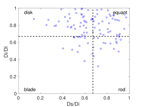
Figure 4: Classification of the shapes of the irregular particles in the a priori test.

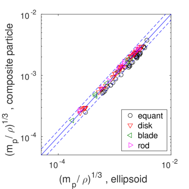
(a) mass

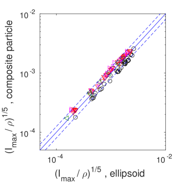
(b) moment of inertia

Figure 5: The mass and moment of inertia of composite irregular particles compared with ellipsoidal particles.

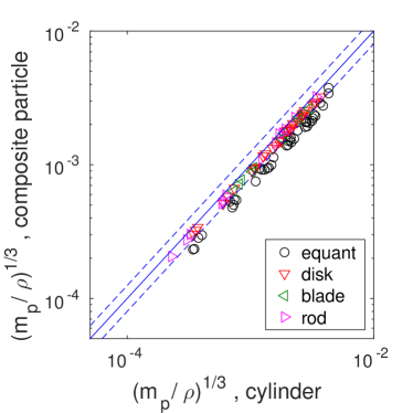
(a) mass

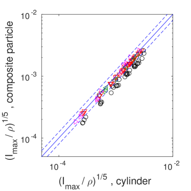
(b) moment of inertia

Figure 6: The mass and moment of inertia of composite irregular particles compared with cylindrical particles.

Another objective of the a priori test is to examine the sedimentation characteristics of the composite particles. To this end, the constructed particles of two representative irregular particles are released in quiescent water at various random initial angles, and their trajectory and change of orientation are observed. It is found that regardless of the initial orientation of the particles when released, they adjust to an orientation where the maximum projection is normal to the fall velocity direction. This is consistent with the experimental observations reported in the literature (Tran-Cong et al., 2004). However, previous authors have also reported the spiral motions and the randomness of particle trajectory (Tran-Cong et al., 2004), which are not observed in our simulations. This is attributed to the fact that the instantaneous shear instability and vortex shedding that lead to spiral motion is not represented in CFD–DEM. Specifically, since the fluid–particle interface is not explicitly resolved in CFD–DEM, only the mean effect of the particle on the flow is represented by applying forces at the cell centers surrounding the particle. However, as with many other dense-phase particle-laden flows, the dynamics of sediment transport is dominated by a number of competing mechanisms such as particle collisions and the associated granular flow dynamics, boundary layer turbulence, and fluid–particle interactions. Therefore, it is not essential or feasible to represent each mechanism exactly. In fact, this compromise is what allows CFD–DEM to handle a much larger number of particle than interface-resolved methods  (Kempe et al., 2014).

Figure 7: The orientation and trajectory of rod- and disk-shaped particles in sedimentation. The red lines are the traces of the center of the composite particle. The particles are enlarged for visualization.

4 Test in Sediment Transport Simulations

Four numerical tests are performed to demonstrate that the proposed method for representing irregular shaped particles is capable of predicting integral quantities in sediment transport applications. The applications include the sedimentation of a single particle in quiescent fluid, the rotation of the irregular particle in boundary layer, the incipient motion of particles, and the sediment transport in a periodic channel. The setup of the numerical tests are based on previous experimental studies (Smith, 2003; Smith and Cheung, 2004, 2005).

The geometry of the simulation is shown in Fig. 8. The dimensions of the domain, the mesh resolutions, and the fluid and particle properties used are detailed in Table 1. Periodic boundary condition is applied in both $x$- and $z$-directions. For the pressure field, zero-gradient boundary condition is applied in $y$-direction; for the velocity field, no-slip wall condition is applied at the bottom in $y$-direction, and slip wall condition is applied on the top. In the sedimentation test, the initial flow is quiescent, and a uniform grid mesh is used. In the rotation test, the fluid flow is driven by a pressure gradient to maintain a constant flow rate $q_{f}$. In addition, different mesh resolutions and boundary conditions are used in the two cases of the rotation test. In the first rotation case, simulations are performed using two meshes: (1) a coarse uniform grid mesh, and (2) a fine mesh refined in the vertical ($y$-) direction towards its bottom boundary. No fixed particles are used at the bottom wall. In the second rotation case, the CFD mesh is refined at the bottom, and three layers of fixed particles are arranged hexagonally to provide a rough bottom boundary condition to the moving particles, as is shown in Fig. 8(b). In the incipient motion test and sediment transport test, the CFD mesh is refined at the bottom, the flow rate is driven by a pressure gradient, and the rough bottom wall is applied. Since detailed size distribution of the irregular particle is not known, the size of irregular particles used in the two tests is uniform. Four example types of bonded particles, shown in Fig. 8(c), represent each type of natural sediment particle, and the proportion of each type is consistent with the measurement by Smith (2003).

(a) sedimentation test

(b) rotation test

(c) incipient motion test and sediment transport test

Figure 8: Layout of the numerical simulations of sediment transport cases: (a) sedimentation test of the terminal velocity, (b) rotation test in boundary layer test, and (c) incipient motion test and sediment transport test. The brown particles are moving irregular particles; the gray particles are fixed particles to provide rough wall boundary conditions. Note that the first case in rotation test are performed without using the rough bottom wall but are not plotted. The particle sizes are not to scale.

Table 1: Parameters of the numerical simulations. The nominal diameter $D_{n}=(D_{l}D_{i}D_{s})^{1/3}$ is used to normalize the dimensions of the computational domain.

	sedimentation test	rotation test	incipient motion test	sediment transport test
domain dimensions
width $(L_{x}/D_{n}$)	10	24	144	144
height $(L_{y}/D_{n}$)	100	20	160	160
transverse thickness $(L_{z}/D_{n}$)	10	12	72	72
mesh resolutions
width $(N_{x})$	10	12	120	120
height $(N_{y})$	100	12 or 30	100	100
transverse thickness $(N_{z})$	10	6	60	60
particle properties
total number of irregular particle	1	1	$6.4\times 10^{4}$	$6.4\times 10^{4}$
nominal diameter $D_{n}$ [mm]	0.7–5.5	0.5	0.2–0.8	0.2–0.8
density $\rho_{s}$ [$\times 10^{3}~{}\mathrm{kg/m^{3}}$]	2650
particle stiffness coefficient [N/m]	20
normal restitution coefficient	0.01
coefficient of friction	0.4
fluid properties
viscosity $\nu$ [$\times 10^{-6}~{}\mathrm{m^{2}/s}$]	1.0	10	1.0	1.0
density $\rho_{f}$ [$\times 10^{3}~{}\mathrm{kg/m^{3}}$]	1.0

4.1 Sedimentation of a Single Particle in Quiescent Flow

The sedimentation test of the constructed particles is performed to show the terminal velocity and drag coefficient of the constructed particles are consistent with the experimental results. The simulations of the sedimentation of 21 irregular particles of various shapes are performed. The nominal diameter $D_{n}=(D_{l}D_{i}D_{s})^{1/3}$ of the constructed particles ranges from 0.7 mm to 5.5 mm according to the experiments conducted by Smith and Cheung (2003). Figure 9 shows the terminal velocity and drag coefficient of constructed particles of different shape factors $S$. The regression curves proposed by Haider and Levenspiel (1989) are used to compare with the results. The shape factor is defined as $S=S_{irregular}/S_{sph}$, where $S_{irregular}$ refers to the surface area of the irregular particle; $S_{sph}$ is the surface area of a spherical particle with the same volume as the irregular particle. Non-dimensional terminal velocity $u^{*}$ is defined as:

$$u^{*}=u_{t}\left(\frac{\rho_{f}^{2}}{g\mu(\rho_{s}-\rho_{f})}\right)^{1/3},$$ (9)

where $u_{t}$ is the terminal velocity of the sediment particles. The non-dimensional particle diameter $d^{*}$ is defined as:

$$d^{*}=D_{n}\left(\frac{g\rho_{f}(\rho_{s}-\rho_{f})}{\mu^{2}}\right)^{1/3},$$ (10)

where the nominal diameter $D_{n}$ is the diameter of the equivalent sphere particle having the same volume. It can be seen in Fig. 9 that the agreement of the terminal velocities and drag coefficients between the numerical simulations and the experimental measurements is good for particles at different shape factors. This indicates the proposed approach of representing irregular particles can capture the decrease of terminal velocity and the increase of drag coefficient compared with spherical particles. In addition, Fig. 9 shows that the scattering of the terminal velocity and drag coefficient is non-negligible for sediment particles at similar size and shape factor. This is because the shape factor is inadequate to describe the settling characteristics of different types of irregular particles. For example, the terminal velocity of rod- and disk-shaped particles of same shape factor can differ significantly. This scattering in terminal velocity and drag coefficient of irregular particles is also observed in previous experimental measurements (Haider and Levenspiel, 1989; Smith and Cheung, 2003).

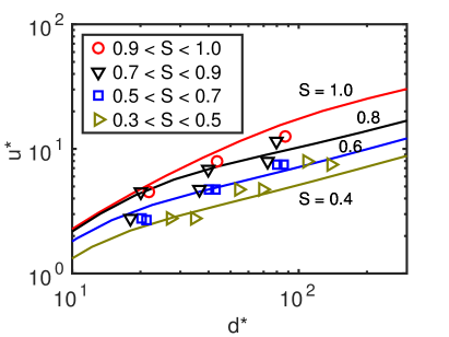
(a) terminal velocity

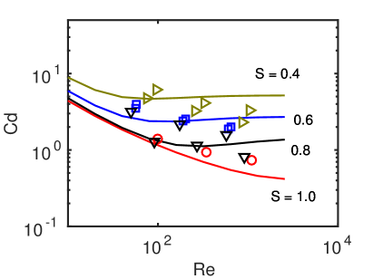
(b) drag coefficient

Figure 9: The terminal velocity and drag coefficient of composite irregular particles of various sizes and shapes: (a) non-dimensional terminal velocity $u^{*}$ plotted as a function of non-dimensional particle diameter $d^{*}$; (b) drag coefficient $C_{d}$ plotted as a function of Reynolds number.

4.2 Translation and Rotation of Particles in Boundary Layer

The motion of irregular particle in the boundary layer is investigated to demonstrate that the proposed approach to represent irregular particle can capture the rotation of sediment particles due to irregularity. Two numerical tests are performed to (1) show the flow velocity gradient is critical to the rotation of irregular particle, and to (2) compare the rotations of different types of irregular particles. In addition, the factors that can influence irregular particle rotation are investigated quantitatively. In the tests, the flow in the periodic channel is laminar at $Re=2000$.

To demonstrate the influence of flow velocity gradient is significant to the rotation of irregular particle, simulations on different mesh resolutions are performed. In the fine mesh test, the flow velocity gradient at the length scale of the composite particle diameter $D_{n}$ is resolved, and the CFD mesh is refined in the vertical direction at the bottom. In the coarse mesh test, the cell size is comparable to the composite particle diameter $D_{n}$, and thus the velocity gradient of the flow at the scale of the particle diameter is not resolved. The predictions of the motion of a disk-shaped particle on meshes of different resolutions are shown in Fig. 10. It can be seen in Fig. 10(a) that the rotation of disk-shaped particle is captured when using fine mesh; whereas Fig. 10(b) shows that the particle is sliding on the bed when coarse mesh is used. The difference in the motion of sediment particles is due to difference of the flow velocity variation $\Delta u=D_{n}\frac{\partial U_{f}}{\partial x}$. When the gradient of flow velocity is resolved using fine mesh, shown in Fig. 10(c), the drag force on the top part of the irregular particle is large and rotates the particle about its center of mass. In contrast, when using coarse mesh, although the flow velocity is large enough to move the sediment particle via the drag forces, the torque excerted on the particle by the flow, as represented by the coarse mesh, is not enough to cause appreciable rotates. This test demonstrates that the proposed method of representing irregular particles can capture the dominant mechanism casuing the particle rotation in the boundary layer.

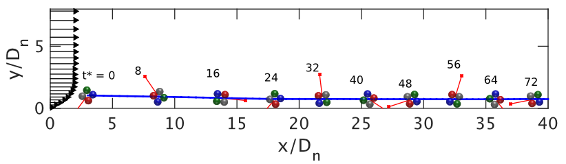
(a) fine mesh

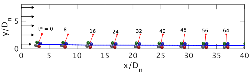
(b) coarse mesh

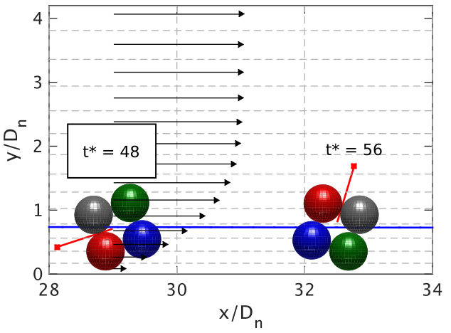
(c) zoom-in view of fine mesh

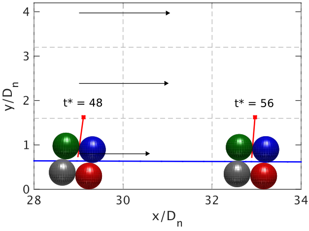
(d) zoom-in view of coarse mesh

Figure 10: The motion of a disk-shaped particle on a smooth bed obtained by using different meshes in laminar flow: (a) fine mesh; (b) coarse mesh; (c) zoom-in view of fine mesh; (d) zoom-in view of coarse mesh. The non-dimensional time is defined as $t^{*}=(t-t_{0})U_{b}/D_{n}$, where $t_{0}$ is the time to start plotting. The arrows indicates the magnitude and direction of the fluid flow. The red flags illustrate the rotation of the disk-shaped particle. The CFD mesh used in the simulations are represented using dashed lines.

In addition, numerical tests are performed on all four types of irregular particles using fine mesh. The purpose of this test is to demonstrate the influence of the particle type to its rotation. The rough wall boundary condition composed of three layers of fixed particles is applied, which is to show the proposed approach can also capture the particle rotation on a rough wall. In this test, the nominal diameters $D_{n}$ of four irregular particles are the same. The snapshots of the rotation of irregular particles are shown in Fig. 11. It can be seen in the figure that the rotation of different types of irregular particles relative to their centers of mass can be captured. From the comparison between Fig. 11(a), (b) and (c) that the rotation velocity of the rod-shaped particle is smaller than that of the disk- and blade-shaped particles. This is because the moment of inertia of rod-shaped particle is relatively larger and thus less likely to rotate compared with disk- and blade-shaped particle. Moreover, it is shown in Fig. 11(d) that the rotation velocity of the equant particle is very small at non-dimensional time $t^{*}=(t-t_{0})U_{b}/D_{n}\in[48,88]$, where $t_{0}$ it the time to start plotting. This can be explained by the fact that the irregularity of the equant particle is relatively small, and thus the torque obtained in boundary flow to drive the rotation of equant particle is also small. Therefore, the rotation velocity of the equant particle is smaller than those of other types with larger irregularity. In addition, it can be seen in Fig. 11 that the velocities of the streamwise transition of different types of particles are not the same. The equant particle, which has the largest shape factor, moves more slowly than other types of irregular particles. This is attributed to the fact that when the irregularity (shape factor $S$) increases, the terminal velocity of the irregular particle increases and the particle is likely to move slower in fluid flow.

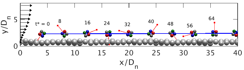
(a) disk-shaped particle

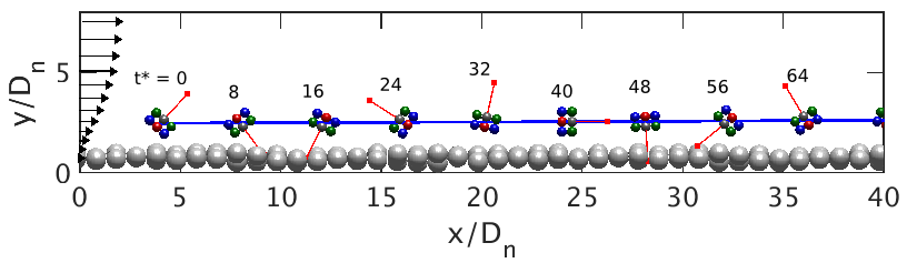
(b) blade-shaped particle

(c) rod-shaped particle

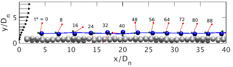
(d) equant particle

Figure 11: The motion of the irregular particle on the rough bottom: (a) composite disk-shaped particle; (b) composite rod-shaped particle; (c) composite blade-shaped particle; (d) composite equant particle. The non-dimensional time is defined as $t^{*}=(t-t_{0})U_{b}/D_{n}$, where $t_{0}$ is the start time to plot. The rought bottom consists of three layers of fixed particles, but only the top layer is plotted.

The numbers of revolutions of the disk-shaped particle plotted as a function of the transitional displacement in streamwise direction are shown in Fig. 12. This aims to investigate the contribution to the particle angular velocity of different factors. The results shown in the figure are obtained in the previous tests: (1) smooth wall and coarse mesh, (2) smooth wall and fine mesh, and (3) rough wall and fine mesh. In all three cases, the particle rotates slowly before it hits the bottom. However, when the disk-shaped particle hits the bottom at $x/D_{n}=40$, the angular velocities of the particles increase significantly. This is because the velocities gradient to drive the particle rotation at the bottom is larger than that in the center of the channel. It can be also seen in the figure that the angular velocity of particle obtained by using fine mesh is much larger than that using coarse mesh. This is attributed to the fact that the contribution of the flow velocity gradient is captured. In addition, the angular velocity of the particle obtained using fine mesh on a rough wall is smaller than that on a smooth wall. This is because the rough wall boundary condition provides more friction than the smooth wall, and thus the angular velocity of the particle is smaller.

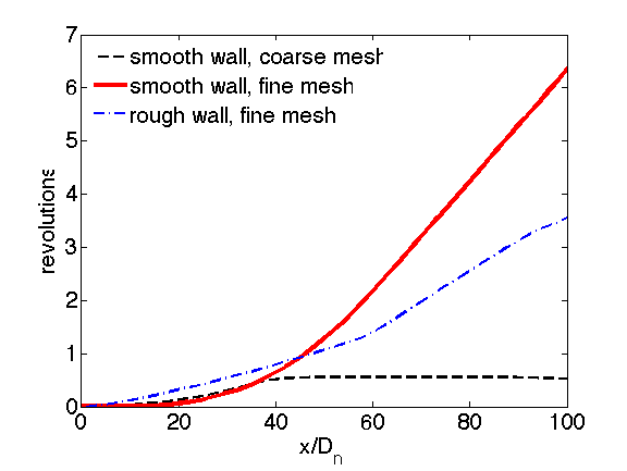
Figure 12: Angle of rotation of the irregular disk-shaped particle in the boundary layer plotted as a function of the non-dimensional transitional displacement in the streamwise direction.

4.3 Incipient Motion

The incipient motion test of the constructed particles is performed to demonstrate that proposed approach to represent irregular particles can capture the initiation of motion of them at critical Shields stress. Three nominal diameters of the irregular particles used in the test are 0.2 mm, 0.5 mm and 0.8 mm, which is according to the particle diameters selected in Smith and Cheung (2004). For each particle diameter, the sediment transport rates obtained at five different velocities (ranging from 0.2 m/s to 0.4 m/s) are plotted as a function of the Shields parameter. To determine the critical Shields parameter in the incipient motion of irregular particles, the threshold transport rate is take as $q*=10^{-4}$ according to Smith and Cheung (2004).

The sediment transport rate plotted as a function of the Shields parameter is shown in Fig. 13(a). It can be seen in the figure that transport rate increases with the Shields parameter for irregular particles at different diameters. The sediment transport rates of small particles are larger than those of larger particles, which is consistent with trend of the experimental data obtained by Smith and Cheung (2004). The critical Shields parameters obtained in the simulations are shown in Fig. 13(b). From the comparison with the experimental measurements (Smith and Cheung, 2004), it can be seen that the proposed approach captures decrease of the critical Shields stress due to the increase of the particle diameter. Moreover, the results obtained in the CFD–DEM simulations are in the range of those obtained by experimental measurements using carbonate sands (Prager et al., 1996). The decrease of the critical Shields parameter in the rough turbulent flow regime ($D_{n}$ = 0.8 mm, $Re_{p}$ = 80) reported by Smith and Cheung (2004) is captured in the simulation. The present approach can capture the decrease of critical Shields parameter because it can predict the increase of the particle drag and the rotation due to particle irregularity, both of which contribute significantly to increase the chance of the incipient motion. On the other hand, the current simulations slightly under-predict the Shields parameter in hydraulic smooth flow regime ($D_{n}$ = 0.2 mm, $Re_{p}$ = 10). From Smith and Cheung (2004), the Shields parameter of irregular particles in this flow regime should be slightly larger than that of spherical particles, which is because the particle irregularity hinders the incipient motion. We argue that the present approach only uses a few spherical particles to represent the irregular particle in consideration of computational cost, and thus the geometric accuracy is not adequate to capture the increase in critical Shields parameter. However, since the under-prediction of the proposed approach is very small, the overall agreement of the Shields parameters reported by the present approach is satisfactory.

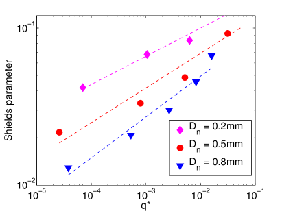
(a) sediment transport rate

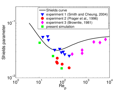
(b) critical Shields parameter

Figure 13: Critical Shields parameters obtained in present simulations. The non-dimensional sediment transport rate is plotted as a function of Shields parameter in Panel (a). The critical Shields parameter plotted as a function of particle Reynolds number $Re_{p}$ in Panel (b).

4.4 Sediment Transport in a Periodic Channel

To test the capability of the proposed approach in the prediction of the sediment transport rate, numerical simulations of sediment transport in a periodic channel are performed. Three nominal diameters of the irregular particles used are 0.2 mm, 0.5 mm and 0.8 mm, which is consistent with the incipient motion test in Section 4.3. The flow velocities in the channel are higher than those in the incipient motion test at 0.4 m/s, 0.5 m/s, and 0.6 m/s. This is because the flow velocities in the sediment transport experiments are higher than those used in incipient motion experiments (Smith and Cheung, 2004, 2005). The proportion of different types of irregular particles is also according to the measurement in Smith (2003). To demonstrate the influence of the particle irregularity to sediment transport, simulations of spherical particle of 0.5 mm are also performed at the same velocities.

Although the setup of the numerical simulations is according to the experimental measurements, the predictions obtained by the numerical approach cannot compare directly to the experimental results. This is because the detailed setup of the experiments in each run is unknown. Therefore, the results from both numerical simulations and experimental measurements are plotted in comparison with the empirical formula proposed by Ackers and White (1973) for validation. The formula proposed by Ackers and White (1973) makes use of the grain-size parameter:

$$D_{*}=D\left[\frac{(s-1)g}{\nu^{2}}\right]^{1/3},$$ (11)

where $D=D_{n}$ is the characteristic grain-size parameter. The sediment transport rate $q$ is defined as:

$$q=B\left(\frac{F}{A}-1\right)^{M}D\bar{u}s\left(\frac{\bar{u}}{u_{*}}\right)^{n},$$ (12)

where $u_{*}$ is the friction velocity; $n$ is the transition parameter given by $n=1-0.56\log(D_{*})$; $\bar{u}$ is depth-averaged flow velocity; $s=\rho_{s}/\rho_{f}$ is the sand specific gravity. The coefficient $F$ denotes the sediment mobility given by:

$$F=\frac{u_{*}^{n}\bar{u}^{1-n}}{\sqrt{gD(s-1)}[\sqrt{32}\log(10d/D)]^{1-n}}.$$ (13)

The initiation of motion is considered in coefficient $A$:

$$A=\frac{0.23}{\sqrt{D_{*}}}+0.14.$$ (14)

The expressions for $B$ and $M$ are updated in Ackers and White (1993):

$$\log(B) =-3.46+2.79\log(D_{*})-0.98\left(\log(D_{*})\right)^{2},$$ (15a)

$$M =\frac{6.83}{D_{*}}+1.67.$$ (15b)

The comparison between sediment transport rates obtained in the simulations and the predictions from the empirical formula in Eq. (12) is shown in Fig. 14. The solid line plotted in the figure indicates perfect agreement; two dash lines of slope 0.5 and 2 indicate under-prediction and over-prediction by a factor of two, respectively. It can be seen in the figure that the results obtained by using spherical particles are consistent with the predictions by the empirical formula. This shows the present CFD–DEM solver can capture the averaged rate of spherical sediment transport in a periodic channel. In addition, most results obtained by using bonded particles are above the solid line, which is consistent with the experimental measurements. This shows that the sediment transport rates of irregular sediment particles are smaller than spherical particles. Comparing the results obtained using both spherical and irregular particles, the present modeling approach captures the influence of particle irregularity which blocks the motion of the irregular particle. Therefore, the proposed algorithm to model irregular sediment particles is capable of predicting bed load sediment transport of irregular particles.

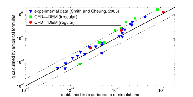
Figure 14: Comparison between the sediment transport rates obtained by using the regression formula in Eq. (12) and those obtained in experimental measurements and numerical simulations.

5 Conclusion

In this work we proposed a simple, efficient approach to represent common sediment grain shapes with composite particles consisting of bonded spheres. The fluid forces are computed and applied on each sphere, which is in contrast to previous works that applied the forces to the center of mass of the composite particle. The proposed approach better represents the fluid-exerted torque on the composite particles, which are important for some forms of sediment transport mode (e.g., saltation) in the bottom boundary layer. Moreover, this method is much simpler and computationally more efficient than representing irregular shaped with non-spherical shapes such as cylinders, ellipsoids, and polygons as pursed in previous works. The simplicity and efficiency are critical for simulating large systems with many particles and offer the flexibility of modeling natural sediments consisting of an arbitrary mixture of particle shapes. Numerical simulations were performed to demonstrate the merits and capability of the proposed method. Specifically, comparison of simulation results with experiments showed that the current method is able to accurately predict the falling characteristics, terminal velocity, threshold of incipient motion, and transport rate of natural sediments. Therefore, the proposed method is a promising approach for faithful representation of natural sediment, which leads to accurate simulations of their transport dynamics.

While this work has focused on non-cohesive sediments, the proposed method also opens the possibility for first-principle-based simulation of the flocculation and sedimentation dynamics of cohesive sediments. Elucidation of these physical mechanisms can provide much needed improvement on the prediction capability and physical understanding of the muddy coasts evolution, which occupy a large portion of the world’s coastlines including tidal flats, slat marshes, lagoons, and estuaries. The method will be applied to the settling and transport of cohesive sediments in future work.

Reference

Appendix A Appendix

Appendix B Representation of Equant Particles

The long, intermediate, and short axes of equant particles have similar length ($\frac{2}{3}D_{l}<D_{i}<D_{l}$ and $\frac{2}{3}D_{i}<D_{s}<D_{i}$). In the proposed method, we attempt to use the smallest number of component spheres to represent each particle and maximize the wetted surface for each component sphere. To this end, the equant particles are further classified to four subtypes, each represented with one main sphere and zero to three auxiliary spheres depending on the particle geometry:

1. Loosely written as $D_{s}\approx D_{i}\approx D_{l}$, the three axes have almost equal lengths as defined by $(1-\varepsilon)D_{l}<D_{i}<D_{l}$ and $(1-\varepsilon)D_{i}<D_{s}<D_{i}$ with $\varepsilon=0.1$, and thus the particle can be considered close to spherical. A single component sphere with diameter $d_{p}=(D_{l}\,D_{i}\,D_{s})^{1/3}$ is used to represent the particle. See Fig. 3(d.1).

2. Loosely written as $D_{s}\approx D_{i}<D_{l}$, the short and intermediate axes have almost equal lengths ($(1-\varepsilon)D_{i}<D_{s}<D_{i}$) but the longer axis is much longer than the intermediate axis ($\frac{2}{3}D_{l}<D_{i}<(1-\varepsilon)D_{l}$). A larger main component sphere of diameter $d_{p,main}=\sqrt{D_{s}D_{i}}$ and a smaller auxiliary component sphere of diameter $d_{p,auxi}=D_{l}-d_{p,main}$ are used to represent the particle. See Fig. 3(d.2).

3. Loosely written as $D_{s}<D_{i}\approx D_{l}$, the long and intermediate axes have almost equal lengths ($(1-\varepsilon)D_{l}<D_{i}<D_{l}$) but the short axis is shorter than the intermediate axis ($\frac{2}{3}D_{i}<D_{s}<(1-\varepsilon)D_{i}$). A larger main component sphere with $d_{p,main}=D_{s}$ and two small auxiliary component spheres with $d_{p,auxi}=D_{l}-D_{s}$ are used to represent the particle. The angle between the auxiliary particles is $\theta_{e}=2\sin^{-1}((D_{i}+D_{s}-D_{l})/D_{l})$. See Fig. 3(d.3).

4. Loosely written as $D_{s}<D_{i}<D_{l}$, neither long and intermediate axes nor intermediate and short axes have almost equal lengths, i.e., ($\frac{2}{3}D_{l}<D_{i}<(1-\varepsilon)D_{l}$) and axis ($\frac{2}{3}D_{i}<D_{s}<(1-\varepsilon)D_{i}$). A larger main component sphere with $d_{p,main}=D_{s}$ and three small auxiliary component spheres with $d_{p,auxi}=0.5(D_{l}-D_{s})$ are used to represent the particle. The arrangement of the sediment particles is shown in Fig. 3(d.4). The main component is aligned with two auxiliary components on both sizes, while angle between the third auxiliary components and the first one is $\theta_{e}=2\sin^{-1}((2D_{i}+D_{s}-D_{l})/(D_{l}+D_{s}))$.

References

- Ackers and White (1973) Ackers, P., White, W. R., 1973. Sediment transport: New approach and analysis. Journal of the Hydraulics Division 99 (11), 2041–2060.
- Ackers and White (1993) Ackers, P., White, W. R., 1993. Sediment transport in open channels: Ackers and White update. Proceedings of the Institution of Civil Engineers, Water, Maritime and Energy 101 (4), 247–249.
- Anderson and Jackson (1967) Anderson, T., Jackson, R., 1967. A fluid mechanical description of fluidized beds: Equations of motion. Industrial and Chemistry Engineering Fundamentals 6, 527–534.
- Ball and Melrose (1997) Ball, R. C., Melrose, J. R., 1997. A simulation technique for many spheres in quasi-static motion under frame-invariant pair drag and Brownian forces. Physica A: Statistical Mechanics and its Applications 247 (1), 444–472.
- Calantoni et al. (2004) Calantoni, J., Holland, K. T., Drake, T. G., 2004. Modelling sheet-flow sediment transport in wave-bottom boundary layers using discrete-element modelling. Philosophical Transactions-Royal Society Of London Series A: Mathematical Physical And Engineering Sciences 362, 1987–2002.
- Capecelatro and Desjardins (2013) Capecelatro, J., Desjardins, O., 2013. An Euler–Lagrange strategy for simulating particle-laden flows. Journal of Computational Physics 238, 1–31.
- Cundall and Strack (1979) Cundall, P., Strack, D., 1979. A discrete numerical model for granular assemblies. Géotechnique 29, 47–65.
- Demir (2000) Demir, T., 2000. The influence of particle shape on bedload transport in coarse-bed river channels. Ph.D. thesis, Durham University.
- Di Felice (1994) Di Felice, R., 1994. The voidage function for fluid-particle interaction systems. International Journal of Multiphase Flow 20 (1), 153–159.
- Favier et al. (1999) Favier, J. F., Abbaspour-Fard, M. H., Kremmer, M., Raji, A. O., 1999. Shape representation of axi-symmetrical, non-spherical particles in discrete element simulation using multi-element model particles. Engineering Computations 16 (4), 467–480.
- Guo et al. (2013) Guo, Y., Wassgren, C., Hancock, B., Ketterhagen, W., Curtis, J., 2013. Granular shear flows of flat disks and elongated rods without and with friction. Physics of Fluids (1994-present) 25 (6), 063304.
- Guo et al. (2012) Guo, Y., Wassgren, C., Ketterhagen, W., Hancock, B., James, B., Curtis, J., 2012. A numerical study of granular shear flows of rod-like particles using the discrete element method. Journal of Fluid Mechanics 713, 1–26.
- Haider and Levenspiel (1989) Haider, A., Levenspiel, O., 1989. Drag coefficient and terminal velocity of spherical and nonspherical particles. Powder technology 58 (1), 63–70.
- Ikeguchi (2004) Ikeguchi, M., 2004. Partial rigid-body dynamics in NPT, NPAT and NPT ensembles for proteins and membranes. Journal of computational chemistry 25 (4), 529–541.
- Issa (1986) Issa, R. I., 1986. Solution of the implicitly discretised fluid flow equations by operator-splitting. Journal of Computational Physics 62 (1), 40–65.
- Kafui et al. (2002) Kafui, K., Thornton, C., Adams, M., 2002. Discrete particle–continuum fluid modelling of gas–solid fluidised beds. Chemical Engineering Science 57 (13).
- Kempe et al. (2014) Kempe, T., Vowinckel, B., Fröhlich, J., 2014. On the relevance of collision modeling for interface-resolving simulations of sediment transport in open channel flow. International Journal of Multiphase Flow 58, 214–235.
- Kodam et al. (2009) Kodam, M., Bharadwaj, R., Curtis, J., Hancock, B., Wassgren, C., 2009. Force model considerations for glued-sphere discrete element method simulations. Chemical Engineering Science 64 (15), 3466–3475.
- Kodam et al. (2010a) Kodam, M., Bharadwaj, R., Curtis, J., Hancock, B., Wassgren, C., 2010a. Cylindrical object contact detection for use in discrete element method simulations. Part I–contact detection algorithms. Chemical Engineering Science 65 (22), 5852–5862.
- Kodam et al. (2010b) Kodam, M., Bharadwaj, R., Curtis, J., Hancock, B., Wassgren, C., 2010b. Cylindrical object contact detection for use in discrete element method simulations, Part II–experimental validation. Chemical Engineering Science 65 (22), 5863–5871.
- Kodam et al. (2012) Kodam, M., Curtis, J., Hancock, B., Wassgren, C., 2012. Discrete element method modeling of bi-convex pharmaceutical tablets: Contact detection algorithms and validation. Chemical Engineering Science 69 (1), 587–601.
- Kruggel-Emden et al. (2008) Kruggel-Emden, H., Rickelt, S., Wirtz, S., Scherer, V., 2008. A study on the validity of the multi-sphere discrete element method. Powder Technology 188 (2), 153–165.
- Krumbein (1941) Krumbein, W. C., 1941. Measurement and geological significance of shape and roundness of sedimentary particles. Journal of Sedimentary Research 11 (2).
- Miller III et al. (2002) Miller III, T., Eleftheriou, M., Pattnaik, P., Ndirango, A., Newns, D., Martyna, G., 2002. Symplectic quaternion scheme for biophysical molecular dynamics. The Journal of chemical physics 116 (20), 8649–8659.
- O’Connor et al. (1997) O’Connor, R., Torczynski, J., Preece, D., Klosek, J., Williams, J., 1997. Discrete element modeling of sand production. International Journal of Rock Mechanics and Mining Sciences 34 (3-4), 1–15.
- OpenCFD (2016) OpenCFD, 2016. OpenFOAM User Guide. See also http://www.opencfd.co.uk/openfoam.
- Plimpton (1995) Plimpton, J., 1995. Fast parallel algorithms for short-range molecular dynamics. Journal of Computational Physics 117, 1–19, see also http://lammps.sandia.gov/index.html.
- Prager et al. (1996) Prager, E. J., Southard, J. B., Vivoni-Gallart, E. R., 1996. Experiments on the entrainment threshold of well-sorted and poorly sorted carbonate sands. Sedimentology 43 (1), 33–40.
- Price et al. (2007) Price, M., Murariu, V., Morrison, G., 2007. Sphere clump generation and trajectory comparison for real particles. In: Proceedings of Fifth International Conference on Discrete Element Methods. August 27–29, Brisbane, Australia.
- Rusche (2003) Rusche, H., 2003. Computational fluid dynamics of dispersed two-phase flows at high phase fractions. Ph.D. thesis, Imperial College London (University of London).
- Saffman (1965) Saffman, P., 1965. The lift on a small sphere in a slow shear flow. Journal of fluid mechanics 22 (02), 385–400.
- Schmeeckle (2014) Schmeeckle, M. W., 2014. Numerical simulation of turbulence and sediment transport of medium sand. Journal of Geophysical Research: Earth Surface 119, 1240–1262.
- Smith (2003) Smith, D. A., 2003. Effect of particle shape on grain size, hydraulic, and transport characteristics of calcareous sand. Ph.D. thesis, University of Hawaii at Manoa.
- Smith and Cheung (2003) Smith, D. A., Cheung, K. F., 2003. Settling characteristics of calcareous sand. Journal of Hydraulic Engineering 129 (6), 479–483.
- Smith and Cheung (2004) Smith, D. A., Cheung, K. F., 2004. Initiation of motion of calcareous sand. Journal of Hydraulic Engineering 130 (5), 467–472.
- Smith and Cheung (2005) Smith, D. A., Cheung, K. F., 2005. Transport rate of calcareous sand in unidirectional flow. Sedimentology 52 (5), 1009–1020.
- Song et al. (2006) Song, Y., Turton, R., Kayihan, F., 2006. Contact detection algorithms for DEM simulations of tablet-shaped particles. Powder Technology 161 (1), 32–40.
- Sun et al. (2007) Sun, J., Battaglia, F., Subramaniam, S., 2007. Hybrid two-fluid DEM simulation of gas-solid fluidized beds. Journal of Fluids Engineering 129 (11), 1394–1403.
- Sun and Xiao (2015a) Sun, R., Xiao, H., 2015a. Diffusion-based coarse graining in hybrid continuum–discrete solvers: Applications in CFD–DEM. International Journal of Multiphase Flow 72, 233–247.
- Sun and Xiao (2015b) Sun, R., Xiao, H., 2015b. Diffusion-based coarse graining in hybrid continuum–discrete solvers: Theoretical formulation and a priori tests. International Journal of Multiphase Flow 77, 142 – 157.
- Sun and Xiao (2016a) Sun, R., Xiao, H., 2016a. CFD–DEM simulations of current-induced dune formation and morphological evolution. Advances in Water Resources 92, 228 – 239.
- Sun and Xiao (2016b) Sun, R., Xiao, H., 2016b. SediFoam: A general-purpose, open-source CFD-DEM solver for particle-laden flow with emphasis on sediment transport. Computers and Geosciences 89, 207–b219.
- Syamlal et al. (1993) Syamlal, M., Rogers, W., O’Brien, T., 1993. MFIX documentation: Theory guide. Tech. rep., National Energy Technology Laboratory, Department of Energy, see also URL http://www.mfix.org.
- Tran-Cong et al. (2004) Tran-Cong, S., Gay, M., Michaelides, E. E., 2004. Drag coefficients of irregularly shaped particles. Powder Technology 139 (1), 21–32.
- Tsuji et al. (1993) Tsuji, Y., Kawaguchi, T., Tanaka, T., 1993. Discrete particle simulation of two-dimensional fluidized bed. Powder Technolgy 77 (79-87).
- van Rijn (1984) van Rijn, L., 1984. Sediment transport, part I: Bed load transport. Journal of hydraulic engineering 110 (10), 1431–1456.
- Wen and Yu (1966) Wen, C., Yu, Y., 1966. Mechanics of fluidization. The Chemical Engineering Progress Symposium Series 162, 100–111.
- Yoshizawa and Horiuti (1985) Yoshizawa, A., Horiuti, K., 1985. A statistically-derived subgrid-scale kinetic energy model for the large-eddy simulation of turbulent flows. Journal of the Physical Society of Japan 54 (8), 2834–2839.
- Zingg (1935) Zingg, T., 1935. Beitrag zur schotteranalyse. Ph.D. thesis, Diss. Naturwiss. ETH Zürich, Nr. 849.