Wavenumber-explicit analysis for the Helmholtz $h$-BEM: error estimates and iteration counts for the Dirichlet problem

Abstract

We consider solving the exterior Dirichlet problem for the Helmholtz equation with the $h$-version of the boundary element method (BEM) using the standard second-kind combined-field integral equations. We prove a new, sharp bound on how the number of GMRES iterations must grow with the wavenumber $k$ to have the error in the iterative solution bounded independently of $k$ as $k\rightarrow\infty$ when the boundary of the obstacle is analytic and has strictly positive curvature. To our knowledge, this result is the first-ever sharp bound on how the number of GMRES iterations depends on the wavenumber for an integral equation used to solve a scattering problem. We also prove new bounds on how $h$ must decrease with $k$ to maintain $k$-independent quasi-optimality of the Galerkin solutions as $k\rightarrow\infty$ when the obstacle is nontrapping.

Keywords: Helmholtz equation, high frequency, boundary integral equation, boundary element method, GMRES, pollution effect, semiclassical

AMS Subject Classifications: 35J05, 35J25, 65N22, 65N38, 65R20

1 Introduction

This paper is concerned with the wavenumber-explicit numerical analysis of boundary integral equations (BIEs) for the Helmholtz equation

$$\Delta u+k^{2}u=0,$$ (1.1)

where $k>0$ is the wavenumber, posed in the exterior of a 2- or 3-dimensional bounded obstacle ${\Omega}$ with Dirichlet boundary conditions on $\Gamma:=\partial{\Omega}$.

We consider the standard second-kind combined-field integral equation formulations of this problem: the so-called “direct” formulation (arising from Green’s integral representation)

$$A^{\prime}_{k,\eta}v=f_{k,\eta}$$ (1.2)

and the so-called “indirect” formulation (arising from an ansatz of layer potentials not related to Green’s integral representation)

$$A_{k,\eta}\phi=g_{k},$$ (1.3)

where

$$A^{\prime}_{k,\eta}:=\frac{1}{2}I+D^{\prime}_{k}-{\rm i}\eta S_{k},\qquad A_{k,\eta}:=\frac{1}{2}I+D_{k}-{\rm i}\eta S_{k},$$ (1.4)

$\eta\in\mathbb{R}\setminus\{0\}$ is an arbitrary coupling parameter, $S_{k}$ is the single-layer operator, $D_{k}$ is the double-layer operator, and $D^{\prime}_{k}$ is the adjoint double-layer operator (1.7), (1.8).

For simplicity of exposition, we focus on the direct equation (1.2), but the main results also hold for the indirect equation (1.3) (see Remark 1.20 below). The contribution to Equation (1.2) from the Dirichlet boundary conditions is contained in the right-hand side $f_{k,\eta}$; our results are independent of the particular form of $f_{k,\eta}$, and so we can simplify the presentation by restricting attention to the particular exterior Dirichlet problem corresponding to scattering by a point source or plane wave, i.e. the sound-soft scattering problem (Definition 1.7 below).

We consider solving the equation (1.2) in ${L^{2}({\partial{\Omega}})}$ using the Galerkin method; this method seeks an approximation $v_{N}$ to the solution $v$ from a finite-dimensional approximation space ${\cal V}_{N}$ (where $N$ is the dimension, i.e. the total number of degrees of freedom). In the majority of the paper $\partial\Omega$ is $C^{2}$, in which case ${\cal V}_{N}$ will be the space of piecewise polynomials of degree $p$, for some fixed $p\geq 0$, on shape-regular meshes of diameter $h$, with $h$ decreasing to zero; this is the so-called $h$–version of the Galerkin method, and we denote ${\cal V}_{N}$ and $v_{N}$ by ${\cal V}_{h}$ and $v_{h}$, respectively, and note that $N\sim h^{-(d-1)}$, where $d$ is the dimension. To find the Galerkin solution $v_{h}$, one must solve a linear system of dimension $N$; in practice this is usually done using Krylov-subspace iterative methods such as the generalized minimal residual method (GMRES).

For the numerical analysis of this situation when $k$ is large, there are now, roughly speaking, two main questions:

1. How must $h$ decrease with $k$ in order to maintain accuracy of the Galerkin solution as $k\rightarrow\infty$?

2. How does the number of GMRES iterations required to achieve a prescribed accuracy grow with $k$?

The goal of this paper is to prove rigorous results about these two questions, and then compare them with the results of numerical experiments.

We now give short summaries of the main results. These results depend on the choice of the coupling parameter $\eta$; for the results on Q1 we need $|\eta|\sim k$ and for the results on Q2 we need $\eta\sim k$, where we use the notation $a\sim b$ to mean that there exists $C_{1},C_{2}>0$, independent of $h$ and $k$, such that $C_{1}b\leq a\leq C_{2}b$. We also use the notation $a\lesssim b$ to mean that there exists $C>0$, independent of $h$ and $k$, such that $a\leq Cb$.

Summary of main results regarding Q1 and their context.

Numerical experiments indicate that, in many cases, the condition $hk\lesssim 1$ is sufficient for the Galerkin method to be quasi-optimal (with the constant of quasi-optimality independent of $k$; i.e., (1.14) below holds); see [44, §5]. This feature can be described by saying that the $h$-BEM does not suffer from the pollution effect (in constrast to the $h$-FEM; see, e.g., [7], [52, Chapter 4]). The best existing result in the literature is that $k$-independent quasi-optimality of the Galerkin method applied to the integral equation (1.2) holds when $hk^{(d+1)/2}\lesssim 1$ for 2- and 3-d $C^{2,\alpha}$ obstacles that are star-shaped with respect to a ball [44, Theorem 1.4]. In this paper we improve this result by showing that the $k$-independent quasioptimality holds for 2-d nontrapping obstacles when $hk^{3/2}\lesssim 1$, for 3-d nontrapping obstacles when $hk^{3/2}\log k\lesssim 1$, and for 2- and 3-d smooth (i.e. $C^{\infty}$) convex obstacles with strictly positive curvature when $hk^{4/3}\lesssim 1$ (see Theorem 1.10 below).

The ideas behind the proofs of these results are summarised in Remark 1.13 below, but we highlight here that all the integral-operator bounds used in these arguments are sharp up to a factor of $\log k$. Therefore, to lower these thresholds on $h$ for which quasi-optimality is proved, one would need to use different arguments than in the present paper. We also highlight that recent experiments by Baydoun and Marburg [60, 10, 61, 11] give examples of Helmholtz problems where the $h$-BEM suffers from a pollution effect, and therefore determining the sharp threshold on $h$ for $k$-independent quasi-optimality to hold in general is an exciting open question.

Summary of main results regarding Q2 and their context.

There has been a large amount of research effort expended on understanding empirically how iteration counts for integral-equation formulations of scattering problems involving the Helmholtz or Maxwell equations depend on $k$; see, e.g, [1, 4, 15, 16, 81], and the references therein.

To our knowledge, however, there are no sharp $k$-explicit bounds in the literature, for any integral-equation formulation of a Helmholtz or Maxwell scattering problem, on the number of iterations GMRES requires to achieve a prescribed accuracy. The main reason, in this current setting of the Helmholtz exterior Dirichlet problem, is that the operator $A^{\prime}_{k,\eta}$ is non-normal for all obstacles other than the circle and sphere [14, 13]. Therefore, for sufficiently-accurate discretisations, the Galerkin matrix of $A^{\prime}_{k,\eta}$ is also non-normal, and one cannot use the well-known bounds on GMRES iterations in terms of the condition number (see, e.g., the review in [71, §6]).

In this paper, we prove that, for 2- and 3-d analytic obstacles with strictly positive curvature, the number of GMRES iterations growing like $k^{1/3}$ is sufficient to have the error in the iterative solution bounded independently of $k$ (see Theorem 1.16 below). Numerical experiments in §5 show that the numbers of GMRES iterations for the sphere and an ellipsoid grow slightly less than $k^{1/3}$ ($k^{0.29}$ for the sphere and $k^{0.28}$ for an ellipsoid), and thus our bound is effectively sharp.

The ideas behind the proof are summarised in Remark 1.18 below. The focus of this paper is in proving results for the operator $A^{\prime}_{k,\eta}$, i.e. the operator in the standard second-kind integral formulation, but we highlight in Remark 4.5 below how a bound on the number of GMRES iterations of $k^{1/2}$ when $d=2$ and $k^{1/2}\log k$ when $d=3$ can be obtained for a modification of $A^{\prime}_{k,\eta}$, the so-called star-combined integral equation introduced in [74]. Moreover, whereas our bound on the number of iterations of $k^{1/3}$ for $A^{\prime}_{k,\eta}$ holds for analytic obstacles with strictly positive curvature, the bounds for the star-combined operator hold for a much wider class of obstacles, namely piecewise-smooth Lipschitz obstacles that are star-shaped with respect to a ball.

Discussion of these results in the context of using semiclassical analysis in the numerical analysis of the Helmholtz equation.

In the last 10 years, there has been growing interest in using results about the $k$-explicit analysis of the Helmholtz equation from semiclassical analysis (a branch of microlocal analysis) to design and analyse numerical methods for the Helmholtz equation. The activity has occurred in, broadly speaking, four different directions:

1. The use of the results of Melrose and Taylor [64] – on the rigorous $k\rightarrow\infty$ asymptotics of the solution of the Helmholtz equation in the exterior of a smooth convex obstacle with strictly positive curvature – to design and analyse $k$-dependent approximation spaces for integral-equation formulations [29, 41, 5, 31, 32, 30],

2. The use of the results of Melrose and Taylor [64], along with the work of Ikawa [53] on scattering from several convex obstacles, to analyse algorithms for multiple scattering problems [33, 2].

3. The use of bounds on the Helmholtz solution operator (also known as resolvent estimates) due to Vainberg [80] (using the propagation of singularities results of Melrose and Sjöstrand [63]) and Morawetz [66] to prove bounds on both $\|(A^{\prime}_{k,\eta})^{-1}\|_{{{L^{2}({\partial{\Omega}})}\rightarrow{L^{2}({\partial{\Omega}})}}}$ and the inf-sup constant of the domain-based variational formulation [22, 73, 9, 24], and also to analyse preconditioning strategies [40].

4. The use of identities originally due to Morawetz [66] to prove coercivity of $A^{\prime}_{k,\eta}$ [75] and to introduce new coercive formulations of Helmholtz problems [74, 65, 42, 43, 28].

The results of the present paper arise from a fifth direction, namely using estimates on the restriction of quasimodes of the Laplacian to hypersurfaces from [79, 17, 77, 48, 26, 78] to prove sharp $k$-explicit bounds on $S_{k},D_{k}$ and $D^{\prime}_{k}$ as operators from ${L^{2}({\partial{\Omega}})}$ to $H^{1}({\partial{\Omega}})$. We state these sharp $k$-explicit bounds in §2 below, and they are proved in the companion paper [39]. In the present paper, we use these new results, in conjunction with the results in Points 3 and 4 above, to obtain answers to Q1 and Q2.

1.1 Formulation of the problem

1.1.1 Geometric definitions.

Let ${\Omega}\subset\mathbb{R}^{d},$ $d=2$ or $3,$ be a bounded Lipschitz open set, such that the open complement ${\Omega_{+}}:=\mathbb{R}^{d}\setminus\overline{{\Omega}}$ is connected. Let $H^{1}_{\text{loc}}(\Omega_{+})$ denote the set of functions $v$ such that $\chi v\in H^{1}(\Omega_{+})$ for every $\chi\in C^{\infty}_{\rm comp}(\overline{\Omega_{+}}):=\{\chi|_{\Omega_{+}}:\,\chi\in C^{\infty}(\mathbb{R}^{d})\text{ is compactly supported}\}$. Let $\gamma^{+}$ denote the trace operator from $\Omega_{+}$ to ${\partial{\Omega}}$. Let $\mathbf{n}$ be the outward-pointing unit normal vector to ${\Omega}$ (i.e. $\mathbf{n}$ points out of ${\Omega}$ and in to ${\Omega_{+}}$), and let $\partial_{n}^{+}$ denote the normal derivative trace operator from ${\Omega_{+}}$ to ${\partial{\Omega}}$ that satisfies $\partial_{n}^{+}u=\mathbf{n}\cdot\gamma^{+}(\nabla u)$ when $u\in H^{2}_{\text{loc}}({\Omega_{+}})$. (We also call $\gamma^{+}u$ the Dirichlet trace of $u$ and $\partial_{n}^{+}u$ the Neumann trace.)

Definition 1.1 (Star-shaped, and star-shaped with respect to a ball)

(i) ${\Omega}$ is star-shaped with respect to the point $\mathbf{x}_{0}\in{\Omega}$ if, whenever $\mathbf{x}\in{\Omega}$, the segment $[\mathbf{x}_{0},\mathbf{x}]\subset{\Omega}$.

(ii) ${\Omega}$ is star-shaped with respect to the ball $B_{a}(\mathbf{x}_{0})$ if it is star-shaped with respect to every point in $B_{a}(\mathbf{x}_{0})$.

(iii) ${\Omega}$ is star-shaped with respect to a ball if there exists $a>0$ and $\mathbf{x}_{0}\in{\Omega}$ such that ${\Omega}$ is star-shaped with respect to the ball $B_{a}(\mathbf{x}_{0})$.

Definition 1.2 (Nontrapping)

We say that ${\Omega}\subset\mathbb{R}^{d},\,d=2,3$ is nontrapping if ${\partial{\Omega}}$ is smooth ($C^{\infty}$) and, given $R$ such that $\overline{{\Omega}}\subset B_{R}(\mathbf{0})$, there exists a $T(R)<\infty$ such that all the billiard trajectories (in the sense of Melrose–Sjöstrand [63, Definition 7.20]) that start in ${\Omega_{+}}\cap B_{R}(\mathbf{0})$ at time zero leave ${\Omega_{+}}\cap B_{R}(\mathbf{0})$ by time $T(R)$.

Definition 1.3 (Smooth hypersurface)

We say that $\Gamma\subset\mathbb{R}^{d}$ is a smooth hypersurface if there exists $\widetilde{\Gamma}$ a compact embedded smooth $d-1$ dimensional submanifold of $\mathbb{R}^{d}$, possibly with boundary, such that $\Gamma$ is an open subset of $\widetilde{\Gamma}$, with $\Gamma$ strictly away from $\partial\widetilde{\Gamma}$, and the boundary of $\Gamma$ can be written as a disjoint union

$$\partial\Gamma=\left(\bigcup_{\ell=1}^{n}Y_{\ell}\right)\cup\Sigma,$$

where each $Y_{\ell}$ is an open, relatively compact, smooth embedded manifold of dimension $d-2$ in $\widetilde{\Gamma}$, $\Gamma$ lies locally on one side of $Y_{\ell}$, and $\Sigma$ is closed set with $d-2$ measure $0$ and $\Sigma\subset\overline{\bigcup_{l=1}^{n}Y_{l}}$. We then refer to the manifold $\widetilde{\Gamma}$ as an extension of $\Gamma$.

For example, when $d=3$, the interior of a 2-d polygon is a smooth hypersurface, with $Y_{i}$ the edges and $\Sigma$ the set of corner points.

Definition 1.4 (Curved)

We say a smooth hypersurface is curved if there is a choice of normal so that the second fundamental form of the hypersurface is everywhere positive definite.

Recall that the principal curvatures are the eigenvalues of the matrix of the second fundamental form in an orthonormal basis of the tangent space, and thus “curved” is equivalent to the principal curvatures being everywhere strictly positive (or everywhere strictly negative, depending on the choice of the normal).

Definition 1.5 (Piecewise smooth)

We say that a hypersurface $\Gamma$ is piecewise smooth if $\Gamma=\cup_{i=1}^{N}\overline{\Gamma}_{i}$ where $\Gamma_{i}$ are smooth hypersurfaces and $\Gamma_{i}\cap\Gamma_{j}=\emptyset.$

Definition 1.6 (Piecewise curved)

We say that a piecewise-smooth hypersurface $\Gamma$ is piecewise curved if $\Gamma$ is as in Definition 1.5 and each $\Gamma_{j}$ is curved.

1.1.2 The boundary value problem and integral equation formulation

Definition 1.7 (Sound-soft scattering problem)

Given $k>0$ and an incident plane wave $u^{I}(\mathbf{x})=\exp({\rm i}k\mathbf{x}\cdot\mathbf{a})$ for some $\mathbf{a}\in\mathbb{R}^{d}$ with $|\mathbf{a}|=1$, find $u^{S}\in C^{2}(\Omega_{+})\cap H^{1}_{\text{\emph{loc}}}(\Omega_{+})$ such that the total field $u:=u^{I}+u^{S}$ satisfies the Helmholtz equation (1.1) in ${\Omega_{+}}$, $\gamma^{+}u=0$ on ${\partial{\Omega}}$, and $u^{S}$ satisfies the Sommerfeld radiation condition

$$\frac{\partial u^{S}}{\partial r}(\mathbf{x})-{\rm i}k\,u^{S}(\mathbf{x})=o\bigg{(}\frac{1}{r^{(d-1)/2}}\bigg{)}$$

as $r:=|\mathbf{x}|\rightarrow\infty$, uniformly in $\mathbf{x}/r$.

The incident field in the sound-soft scattering problem of Definition 1.7 is a plane wave, but this could be replaced by a point source or, more generally, a solution of the Helmholtz equation in a neighbourhood of $\Omega$; see [19, Definition 2.11].

Obtaining the direct integral equation (1.2).

If $u$ satisfies the sound-soft scattering problem of Definition 1.7 then Green’s integral representation implies that

$$u(\mathbf{x})=u^{I}(\mathbf{x})-\int_{\partial{\Omega}}\Phi_{k}(\mathbf{x},\mathbf{y})\partial_{n}^{+}u(\mathbf{y})\,{\rm d}s(\mathbf{y}),\quad\mathbf{x}\in{\Omega_{+}},$$ (1.5)

(see, e.g., [19, Theorem 2.43]), where $\Phi_{k}(\mathbf{x},\mathbf{y})$ is the fundamental solution of the Helmholtz equation given by

$$\Phi_{k}(\mathbf{x},\mathbf{y})=\displaystyle\frac{{\rm i}}{4}H_{0}^{(1)}\big{(}k|\mathbf{x}-\mathbf{y}|\big{)},\,\,d=2,\quad\quad\Phi_{k}(\mathbf{x},\mathbf{y})=\frac{{\rm e}^{{\rm i}k|\mathbf{x}-\mathbf{y}|}}{4\pi|\mathbf{x}-\mathbf{y}|},\,\,d=3$$

(note that we have chosen the sign of $\Phi_{k}(\mathbf{x},\mathbf{y})$ so that $-(\Delta+k^{2})\Phi_{k}(\mathbf{x},\mathbf{y})=\delta(\mathbf{x}-\mathbf{y})$). Taking the exterior Dirichlet and Neumann traces of (1.5) on ${\partial{\Omega}}$ and using the jump relations for the single- and double-layer potentials (see, e.g., [19, Equation 2.41]) we obtain the integral equations

$$S_{k}\partial_{n}^{+}u=\gamma^{+}u^{I}\quad\text{ and }\quad\left(\frac{1}{2}I+D_{k}^{\prime}\right)\partial_{n}^{+}u=\partial_{n}^{+}u^{I},$$ (1.6)

where $S_{k}$ and $D^{\prime}_{k}$ are the single- and adjoint-double-layer operators defined by

$$S_{k}\phi(\mathbf{x}):= \int_{\partial{\Omega}}\Phi_{k}(\mathbf{x},\mathbf{y})\phi(\mathbf{y})\,{\rm d}s(\mathbf{y}),\quad D^{\prime}_{k}\phi(\mathbf{x}):=\int_{\partial{\Omega}}\frac{\partial\Phi_{k}(\mathbf{x},\mathbf{y})}{\partial n(\mathbf{x})}\phi(\mathbf{y})\,{\rm d}s(\mathbf{y}),$$ (1.7)

for $\phi\in{L^{2}({\partial{\Omega}})}$ and $x\in{\partial{\Omega}}$. Later we will also need the definition of the double-layer potential,

$$D_{k}\phi(\mathbf{x}):=\int_{\partial{\Omega}}\frac{\partial\Phi_{k}(\mathbf{x},\mathbf{y})}{\partial n(\mathbf{y})}\phi(\mathbf{y})\,{\rm d}s(\mathbf{y})\quad\text{ for }\phi\in{L^{2}({\partial{\Omega}})}\,\text{ and }\,\mathbf{x}\in{\partial{\Omega}}.$$ (1.8)

The first equation in (1.6) is not uniquely solvable when $-k^{2}$ is a Dirichlet eigenvalue of the Laplacian in ${\Omega}$, and the second equation in (1.6) is not uniquely solvable when $-k^{2}$ is a Neumann eigenvalue of the Laplacian in ${\Omega}$ (see, e.g., [19, Theorem 2.25]). The standard way to resolve this difficulty is to take a linear combination of the two equations, which yields the integral equation (1.2) where $A^{\prime}_{k,\eta}$ is defined by (1.4),

$$f_{k,\eta}:=\partial_{n}^{+}u^{I}-{\rm i}\eta\,\gamma^{+}u^{I},$$ (1.9)

and we use the notation that $v:=\partial_{n}^{+}u$ (this makes denoting the Galerkin solution below easier, since we then have $v_{h}$ instead of $(\partial_{n}^{+}u)_{h}$).

The space ${L^{2}({\partial{\Omega}})}$ is a natural space for the practical solution of second-kind integral equations since it is self-dual, and, for $\eta\in\mathbb{R}\setminus\{0\}$, $A^{\prime}_{k,\eta}$ is a bounded invertible operator from ${L^{2}({\partial{\Omega}})}$ to itself [19, Theorem 2.27]. Furthermore the right-hand side $f_{k,\eta}$ is in ${L^{2}({\partial{\Omega}})}$ (since $u^{I}\in C^{\infty}(\overline{{\Omega_{+}}})$) and thus we consider the equation (1.2) as an equation in ${L^{2}({\partial{\Omega}})}$.

The Galerkin method.

Given a finite-dimensional approximation space ${\cal V}_{N}\subset{L^{2}({\partial{\Omega}})}$, the Galerkin method for the integral equation (1.2) is

$$\text{find }v_{N}\in{\cal V}_{N}\text{ such that }\,\big{(}A^{\prime}_{k,\eta}v_{N},w_{N}\big{)}_{{L^{2}({\partial{\Omega}})}}=\big{(}f_{k,\eta},w_{N}\big{)}_{{L^{2}({\partial{\Omega}})}}\,\text{ for all }w_{N}\in{\cal V}_{N}.$$ (1.10)

Let ${\cal V}_{N}=\mathop{{\rm span}}\{\phi_{i}:i=1,\ldots,N\}$, let $v_{N}\in{\cal V}_{N}$ be equal to $\sum_{j=1}^{N}V_{j}\phi_{j}$, and define $\mathbf{v}\in\mathbb{C}^{N}$ by $\mathbf{v}:=(V_{j})_{j=1}^{N}$. Then, with $\mathbf{A}_{ij}:=(A^{\prime}_{k,\eta}\phi_{j},\phi_{i})_{{L^{2}({\partial{\Omega}})}}$ and $\mathbf{f}_{i}:=(f_{k,\eta},\phi_{i})_{{L^{2}({\partial{\Omega}})}}$, the Galerkin method (1.10) is equivalent to solving the linear system $\mathbf{A}\mathbf{v}=\mathbf{f}$.

We consider the $h$–version of the Galerkin method, and we then denote ${\cal V}_{N}$ and $v_{N}$ by ${\cal V}_{h}$ and $v_{h}$ respectively. The main results for Q1 and Q2 will be stated under the following assumption on ${\cal V}_{h}$.

Assumption 1.8 (Assumptions on ${\cal V}_{h}$)

${\cal V}_{h}$ is a space of piecewise polynomials of degree $p$ for some fixed $p\geq 0$ on shape-regular meshes of diameter $h$, with $h$ decreasing to zero (see, e.g., [70, Chapter 4] for specific realisations). Furthermore

(a) if $w\in H^{1}({\partial{\Omega}})$ then

$$\min_{w_{h}\in{\cal V}_{h}}\left\|w-w_{h}\right\|_{{L^{2}({\partial{\Omega}})}}\lesssim h\left\|w\right\|_{H^{1}({\partial{\Omega}})},$$ (1.11)

(b)

$$\left\|w_{h}\right\|^{2}_{{L^{2}({\partial{\Omega}})}}\sim h^{d-1}\left\|\mathbf{w}\right\|_{2}^{2},$$ (1.12)

where $\|\cdot\|_{2}$ denotes the $l_{2}$ (i.e. euclidean) vector norm.

Remark 1.9 (For what situations is Assumption 1.8 proved?)

Part (a) is proved for subspaces consisting of piecewise-constant basis functions in [70, Theorem 4.3.19] when ${\partial{\Omega}}$ is a polyhedron or curved (in the sense of Assumptions 4.3.17 and 4.3.18, respectively, in [70]) and in [76, Theorem 10.4] when ${\Omega}$ is a piecewise-smooth Lipschitz domain. Part (a) is proved for subspaces consisting of continuous piecewise-polynomials of degree $p\geq 1$ (in the sense of [70, Definition 4.1.36]) in [70, Theorem 4.3.28].

Part (b) is proved for subspaces consisting of piecewise-linear basis function in [76, Lemma 10.5] when ${\partial{\Omega}}$ is piecewise-smooth and Lipschitz, and for more general subspaces in [70, Theorem 4.4.7].

1.2 Statement of the main results and discussion

The results concerning Q1 are stated in §1.2.1, and the results concerning Q2 are stated in §1.2.2.

1.2.1 Results concerning Q1

Theorem 1.10 (Sufficient conditions for the Galerkin method to be quasi-optimal)

Let $u$ be the solution of the sound-soft scattering problem of Definition 1.7 and let $v:=\partial_{n}^{+}u$. Let $|\eta|\sim k$, and let ${\cal V}_{h}$ satisfy Part (a) of Assumption 1.8.

(a) If either (i) ${\Omega}$ is nontrapping, or (ii) ${\Omega}$ is star-shaped with respect to a ball and ${\partial{\Omega}}$ is $C^{2,\alpha}$ and piecewise smooth, then given $k_{0}>0$, there exists a $C>0$ (independent of $k$ and $h$) such that if

$$hk^{3/2}\leq C,\quad d=2,\quad hk^{3/2}\log k\leq C,\quad d=3,$$ (1.13)

then the Galerkin equations (1.10) have a unique solution which satisfies

$$\left\|v-v_{h}\right\|_{{L^{2}({\partial{\Omega}})}}\lesssim\min_{w_{h}\in{\cal V}_{h}}\left\|v-w_{h}\right\|_{{L^{2}({\partial{\Omega}})}}$$ (1.14)

for all $k\geq k_{0}$.

(b) In case (ii) above, if additionally ${\partial{\Omega}}$ is piecewise curved, then given $k_{0}>0$, there exists a $C>0$ (independent of $k$ and $h$) such that if

$$hk^{4/3}\log k\leq C,\quad d=2,3$$ (1.15)

then (1.14) holds.

(c) If ${\Omega}$ is convex and ${\partial{\Omega}}$ is $C^{\infty}$ and curved then given $k_{0}>0$, there exists a $C>0$ (independent of $k$ and $h$) such that if

$$hk^{4/3}\leq C,\quad d=2,3$$ (1.16)

then (1.14) holds.

Having established quasi-optimality, it is then natural to ask how the best approximation error $\min_{w_{h}\in{\cal V}_{h}}\left\|v-w_{h}\right\|_{{L^{2}({\partial{\Omega}})}}$ depends on $k$, $h$, and $\|v\|_{L^{2}({\partial{\Omega}})}$.

Theorem 1.11 (Bounds on the best approximation error)

Let $u$ be the solution of the sound-soft scattering problem of Definition 1.7 and let $v:=\partial_{n}^{+}u$. Let ${\cal V}_{h}$ satisfy Assumption 1.8.

(a) If ${\partial{\Omega}}$ is $C^{2,\alpha}$ and piecewise smooth, then, given $k_{0}>0$,

$$\min_{w_{h}\in{\cal V}_{h}}\left\|v-w_{h}\right\|_{{L^{2}({\partial{\Omega}})}}\lesssim hA(k)\left\|v\right\|_{{L^{2}({\partial{\Omega}})}}$$ (1.17)

with $A(k)=k^{5/4}\log k$, for all $k\geq k_{0}$.

(b) If ${\partial{\Omega}}$ is piecewise curved, then, given $k_{0}>0$, (1.17) holds with $A(k)=k^{7/6}\log k$, for all $k\geq k_{0}$.

(c) If ${\Omega}$ is convex and ${\partial{\Omega}}$ is $C^{\infty}$ and curved, then, given $k_{0}>0$, (1.17) holds with $A(k)=k$, for all $k\geq k_{0}$.

Combining Theorems 1.10 and 1.11 we can obtain bounds on the relative error of the Galerkin method. For brevity, we only state the ones corresponding to cases (a) and (c) in Theorems 1.10 and 1.11.

Corollary 1.12 (Bound on the relative errors in the Galerkin method)

Let $u$ be the solution to the sound-soft scattering problem, let $|\eta|\sim k$, and let ${\cal V}_{h}$ satisfy Part (a) of Assumption 1.8.

(a) If either (i) ${\Omega}$ is nontrapping, or (ii) ${\Omega}$ is star-shaped with respect to a ball and ${\partial{\Omega}}$ is $C^{2,\alpha}$ and piecewise smooth, then given $k_{0}>0$, there exists a $C>0$ (independent of $k$ and $h$) such that if $h$ and $k$ satisfy (1.13) then the Galerkin equations (1.10) have a unique solution which satisfies

$$\frac{\left\|v-v_{h}\right\|_{{L^{2}({\partial{\Omega}})}}}{\left\|v\right\|_{{L^{2}({\partial{\Omega}})}}}\lesssim\begin{cases}k^{-1/4}\log k,&d=2,\\ k^{-1/4},&d=3,\end{cases}$$

for all $k\geq k_{0}$.

(b) If ${\Omega}$ is convex and ${\partial{\Omega}}$ is $C^{\infty}$ and curved, then given $k_{0}>0$, there exists a $C>0$ (independent of $k$ and $h$) such that if $hk^{4/3}\leq C$ the Galerkin equations (1.10) have a unique solution which satisfies

$$\frac{\left\|v-v_{h}\right\|_{{L^{2}({\partial{\Omega}})}}}{\left\|v\right\|_{{L^{2}({\partial{\Omega}})}}}\lesssim\frac{1}{k^{1/3}}$$

for all $k\geq k_{0}$.

Remark 1.13 (The main ideas behind the proofs of Theorems 1.10 and 1.11)

The proof of Theorem 1.10 uses the classic projection-method analysis of second-kind integral equations (see, e.g., [6, Chapter 3]), with $A^{\prime}_{k,\eta}$ treated as a compact perturbation of $\frac{1}{2}I$. In [44], this argument was used to reduce the question of finding $k$-explicit bounds on the mesh threshold $h$ for $k$-independent quasi-optimality to hold to finding $k$-explicit bounds on

$$\|S_{k}\|_{{L^{2}({\partial{\Omega}})}\rightarrow H^{1}({\partial{\Omega}})},\quad\|D^{\prime}_{k}\|_{{L^{2}({\partial{\Omega}})}\rightarrow H^{1}({\partial{\Omega}})},\quad\text{ and }\quad\|(A^{\prime}_{k,\eta})^{-1}\|_{{{L^{2}({\partial{\Omega}})}\rightarrow{L^{2}({\partial{\Omega}})}}}.$$

We use the new, sharp bounds on the first two of these norms from [39], quoted here as Theorem 2.1, and the sharp bounds on the third of these norms from [9, Theorem 1.13] (for nontrapping obstacles) and [22, Theorem 4.3] (for obstacles that are star-shaped with respect to a ball).

The bounds of Theorem 1.11 are proved by showing that

$$\left\|v\right\|_{H^{1}({\partial{\Omega}})}\lesssim A(k)\left\|v\right\|_{{L^{2}({\partial{\Omega}})}},$$ (1.18)

and then using the approximation theory result (1.11). The bound (1.18) is obtained from the integral equation (1.2) using the second-kind-structure of the equation and the ${L^{2}({\partial{\Omega}})}\rightarrow H^{1}({\partial{\Omega}})$ bounds on $S_{k}$ and $D^{\prime}_{k}$ from Theorem 2.1.

Remark 1.14 (Comparison to previous results)

Theorems 1.10 and 1.11 and Corollary 1.12 sharpen previous results in [44]: the mesh thresholds for quasi-optimality in Theorem 1.10 are sharper than the corresponding ones in [44], and the results are valid for a wider class of obstacles.

This sharpening is due to the new, sharp bounds on ${L^{2}({\partial{\Omega}})}\rightarrow H^{1}({\partial{\Omega}})$ norms of $S_{k}$, $D_{k}$, and $D^{\prime}_{k}$ from [39], and the widening of the class of obstacles is due to the bound on $\|(A^{\prime}_{k,\eta})^{-1}\|_{{{L^{2}({\partial{\Omega}})}\rightarrow{L^{2}({\partial{\Omega}})}}}$ for nontrapping obstacles from [9, Theorem 1.13]. In more detail: Theorem 1.4 of [44] is the analogue of our Theorem 1.10 except that the former is only valid when ${\Omega}$ is star-shaped with respect to a ball and $C^{2,\alpha}$ and the mesh threshold is $hk^{(d+1)/2}\leq C$. Comparing this result to Theorem 1.10 we see that we’ve sharpened the threshold in the $d=3$ case, expanded the class of obstacles to nontrapping ones, and added the additional results (b) and (c). Theorem 1.11 on the best approximation error is again proved using the ${L^{2}({\partial{\Omega}})}\rightarrow H^{1}({\partial{\Omega}})$-bounds from [39] and thus we see similar improvements over the corresponding theorem in [44] ([44, Theorem 1.3]).

As discussed in Remark 1.13, both the present paper and [44] use the classic projection-method argument to obtain $k$-explicit results about quasi-optimality of the $h$-BEM. There are two other sets of results about quasi-optimality of the $h$-BEM in the literature:

1. results that use coercivity [29, 74, 75], and

2. results that give sufficient conditions for quasi-optimality to hold in terms of how well the spaces ${\cal V}_{h}$ approximate the solution of certain adjoint problems [8, 57, 62].

These two sets of results are discussed in detail in [44, pages 181–182] and [44, §4.2] respectively, and neither give results as strong as those in Theorem 1.10.

Finally, in this paper we have only considered the $h$-BEM; a thorough $k$-explicit analysis of the $hp$-BEM for the exterior Dirichlet problem was conducted in [57] and [62]. In particular, this analysis, combined with the bound on $\|(A^{\prime}_{k,\eta})^{-1}\|_{{{L^{2}({\partial{\Omega}})}\rightarrow{L^{2}({\partial{\Omega}})}}}$ for nontrapping obstacles from [9, Theorem 1.13], proves that $k$-independent quasi-optimality can be obtained for nontrapping obstacles through a choice of $h$ and $p$ that keeps the total number of degrees of freedom proportional to $k^{d-1}$ [57, Corollaries 3.18 and 3.19].

Remark 1.15 (How sharp are the quasioptimality results?)

Numerical experiments in [44, §5] show that for a wide variety of obstacles (including certain mildly-trapping obstacles) the $h$-BEM is quasi-optimal with constant independent of $k$ (i.e. (1.14) holds), when $hk\sim 1$. The closest we can get to proving this is the result for strictly convex obstacles in Theorem 1.10 part (c), with the threshold being $hk^{4/3}\leq C$. The recent results of Baydoun and Marburg [60, 10, 61, 11], however, give examples of cases where $hk\sim 1$ is not sufficient to keep the error bounded as $k\rightarrow\infty$.

1.2.2 Result concerning Q2

We now consider solving the linear system $\mathbf{A}\mathbf{v}=\mathbf{f}$ with the generalised minimum residual method (GMRES) introduced by Saad and Schultz in [69]; for details of the implementation of this algorithm, see, e.g., [68, 45].

Theorem 1.16 (A bound on the number of GMRES iterations)

Let ${\Omega}$ be a 2- or 3-d convex obstacle whose boundary ${\partial{\Omega}}$ is analytic and curved. Let ${\cal V}_{h}$ satisfy Part (b) of Assumption 1.8, let the Galerkin matrix corresponding to (1.10) be denoted by $\mathbf{A}$, and consider GMRES applied to $\mathbf{A}\mathbf{v}=\mathbf{f}$

There exist constants $\eta_{0}>0$ and $k_{0}>0$ (with $\eta_{0}=1$ if $\Omega$ is a ball) such that if $k\geq k_{0}$ and $\eta_{0}k\leq\eta\lesssim k$, then, given $0<\varepsilon<1$, there exists a $C$ (independent of $k$, $\eta$, and $\varepsilon$) such that if

$$m\geq Ck^{1/3}\log\left(\frac{12}{\varepsilon}\right),$$ (1.19)

then the $m$th GMRES residual $\mathbf{r}_{m}:=\mathbf{A}\mathbf{v}_{m}-\mathbf{f}$ satisfies

$$\frac{\left\|\mathbf{r}_{m}\right\|_{2}}{\left\|\mathbf{r}_{0}\right\|_{2}}\leq\varepsilon,$$

where $\|\cdot\|_{2}$ denotes the $l_{2}$ (i.e. euclidean) vector norm.

In other words, Theorem 1.16 states that, for convex, analytic, curved $\Omega$, the number of iterations growing like $k^{1/3}$ is a sufficient condition for GMRES to maintain accuracy as $k\rightarrow\infty$.

Remark 1.17 (How sharp is the result of Theorem 1.16?)

Numerical experiments in §5 show that for the sphere the number of GMRES iterations grows like $k^{0.29}$, and for an ellipsoid they grow like $k^{0.28}$. The bound in Theorem 1.16 is therefore effectively sharp (at least for the range of $k$ considered in the experiments).

Remark 1.18 (The main ideas behind the proof of Theorem 1.16)

The two ideas behind Theorem 1.16 are that:

(a) A sufficient (but not necessary) condition for iterative methods to be well behaved is that the numerical range (also known as the field of values) of the matrix is bounded away from zero, and in this case the Elman estimate [35, 34] and its refinement due to Beckermann, Goreinov, and Tyrtyshnikov [12] can be used to bound the number of GMRES iterations in terms of (i) the distance of the numerical range to the origin, and (ii) the norm of the matrix.

(b) When ${\Omega}$ is convex, $C^{3}$, piecewise analytic, and ${\partial{\Omega}}$ is curved, [75] proved that $A^{\prime}_{k,\eta}$ is coercive for sufficiently large $k$ (with $\eta\sim k$). The $k$-dependence of the coercivity constant, along with the $k$-dependence of $\|A^{\prime}_{k,\eta}\|_{{L^{2}({\partial{\Omega}})}\rightarrow{L^{2}({\partial{\Omega}})}}$ then give the information needed about the numerical range of the Galerkin matrix $\mathbf{A}$ required in (a).

Remark 1.19 (Comparison to previous results)

The bound $m\gtrsim k^{2/3}$ when ${\partial{\Omega}}$ is a sphere was stated in [75, §1.3]; this bound was obtained using the original Elman estimate (see Remark 4.4 below), and the fact that the sharp bound $\|A^{\prime}_{k,\eta}\|_{{{L^{2}({\partial{\Omega}})}\rightarrow{L^{2}({\partial{\Omega}})}}}\lesssim k^{1/3}$ was known for the circle and sphere; see [19, §5.4]. To our knowledge, there are no other $k$-explicit bounds in the literature on the number of GMRES iterations required to achieve a prescribed accuracy for a Helmholtz BIE. The closest related work is [23], which uses a second-kind integral equation to solve the Helmholtz equation in a half-plane with an impedance boundary condition. The special structure of this integral equation allows a two-grid iterative method to be used, and [23] proves that there exists $C>0$ such that if $kh\leq C$, then, after seven iterations, the difference between the solution and the Galerkin solution computed via the iterative method is bounded independently of $k$ and $h$.

Remark 1.20 (Translating the results to the indirect equation (1.3))

Instead of using Green’s integral representation (1.5) to formulate the sound-soft scattering problem as the integral equation (1.2), one can pose the ansatz that the scattered field satisfies

$$u^{S}(\mathbf{x})=\int_{\partial{\Omega}}\frac{\partial\Phi_{k}(\mathbf{x},\mathbf{y})}{\partial n(\mathbf{y})}\phi(\mathbf{y})\,{\rm d}s(\mathbf{y})-{\rm i}\eta\int_{\partial{\Omega}}\Phi_{k}(\mathbf{x},\mathbf{y})\phi(\mathbf{y})\,{\rm d}s(\mathbf{y})$$

for $\mathbf{x}\in{\Omega_{+}}$, $\phi\in{L^{2}({\partial{\Omega}})}$, and $\eta\in\mathbb{R}\setminus\{0\}$. Imposing the boundary condition $\gamma^{+}u^{S}=-\gamma^{+}u^{I}$ on ${\partial{\Omega}}$ and using the jump relations for the single- and double-layer potentials leads to the integral equation (1.3) where $A_{k,\eta}$ is defined by (1.4) and $g=-\gamma^{+}u^{I}$. One can show that $A_{k,\eta}$ and $A^{\prime}_{k,\eta}$ are adjoint with respect to the real-valued ${L^{2}({\partial{\Omega}})}$ inner product (see, e.g., [19, Equation 2.37, Remark 2.24, §2.6]), and so their norms are equal, the norms of their inverses are equal, and if one is coercive then so is the other (with the same coercivity constant). These facts imply that the results of Theorems 1.10 and Theorem 1.16 hold for the indirect equation (1.3).

The bounds on the best approximation error in Theorem 1.11 hold for the indirect equation (1.3) with (a) $A(k)=k^{3/2}$ for $d=2$, $A(k)=k^{3/2}\log k$ for $d=3$, (b) $A(k)=k^{4/3}\log k$, and (c) $A(k)=k^{4/3}$. These powers of $k$ are all slightly higher than those for the direct equation; the reason for this is that we have more information about the unknown in the direct equation (since it is $\partial_{n}^{+}u$) than about the unknown $\phi$ in the indirect equation. Indeed, one can express $\phi$ in terms of the difference of solutions to interior and exterior boundary value problems – see [19, Page 132] – but it is harder to make use of this fact than for the direct equation.

Remark 1.21 (Translating the results to the general exterior Dirichlet problem)

The results of Theorems 1.10 and 1.16 are independent of the right-hand side of the integral equation (1.2), and therefore hold for the general Dirichlet problem with Dirichlet data in $H^{1}({\partial{\Omega}})$ (this assumption is needed so that $A^{\prime}_{k,\eta}$ can still be considered as an operator on ${L^{2}({\partial{\Omega}})}$; see, e.g., [19, §2.6]). The results of Theorem 1.11 and Corollary 1.12, however, do not immediately hold for the general Dirichlet problem, since they use the particular form of the right-hand side in (1.9).

Outline of the paper

In §2 we recap the sharp ${L^{2}({\partial{\Omega}})}\rightarrow H^{1}({\partial{\Omega}})$ bounds from the companion paper [39]. In §3 we prove Theorems 1.10 and 1.11 (the results concerning Q1). In §4 we prove Theorem 1.16 (the result concerning Q2), and then in §5 we give numerical experiments showing that Theorem 1.16 is effectively sharp in its $k$-dependence.

2 Recap of the ${L^{2}({\partial{\Omega}})}\rightarrow H^{1}({\partial{\Omega}})$ bounds from [39]

The following result was proved in [39, Theorem 2.10]. In stating this result, we use the weighted $H^{1}({\partial{\Omega}})$ norm

$$\left\|w\right\|_{H^{1}_{k}({\partial{\Omega}})}^{2}:=k^{-2}\left\|\nabla_{{\partial{\Omega}}}w\right\|_{{L^{2}({\partial{\Omega}})}}^{2}+\left\|w\right\|_{{L^{2}({\partial{\Omega}})}}^{2},$$ (2.1)

in contrast to the usual $H^{1}({\partial{\Omega}})$ norm

$$\left\|w\right\|_{H^{1}({\partial{\Omega}})}^{2}:=\left\|\nabla_{{\partial{\Omega}}}w\right\|_{{L^{2}({\partial{\Omega}})}}^{2}+\left\|w\right\|_{{L^{2}({\partial{\Omega}})}}^{2},$$

where $\nabla_{{\partial{\Omega}}}$ is the surface gradient operator on ${\partial{\Omega}}$ (see, e.g., [19, Page 276]); we note that the use of such weighted norms is standard in both the semiclassical and numerical analysis of the Helmholtz equation, and reflects the fact that we expect to incur a power of $k$ every time we take a derivative of a Helmholtz solution; see, e.g., [65, Remark 3.8].

Theorem 2.1 (Bounds on $\|S_{k}\|_{{L^{2}({\partial{\Omega}})}\rightarrow H^{1}_{k}({\partial{\Omega}})}$, $\|D_{k}\|_{{L^{2}({\partial{\Omega}})}\rightarrow H^{1}_{k}({\partial{\Omega}})}$, $\|D^{\prime}_{k}\|_{{L^{2}({\partial{\Omega}})}\rightarrow H^{1}_{k}({\partial{\Omega}})}$)

Let $\Omega$ be a bounded Lipschitz open set such that the open complement ${\Omega_{+}}:=\mathbb{R}^{d}\setminus\overline{\Omega}$ is connected.

(a) If ${\partial{\Omega}}$ is a piecewise-smooth hypersurface (in the sense of Definition 1.5), then, given $k_{0}>1$, there exists $C>0$ (independent of $k$) such that

$$\|S_{k}\|_{L^{2}({\partial{\Omega}})\to H_{k}^{1}({\partial{\Omega}})}\leq C\,k^{-1/2}\,\log k.$$ (2.2)

for all $k\geq k_{0}$. Moreover, if ${\partial{\Omega}}$ is piecewise curved (in the sense of Definition 1.6), then, given $k_{0}>1$, the following stronger estimate holds for all $k\geq k_{0}$

$$\left\|S_{k}\right\|_{{L^{2}({\partial{\Omega}})}\rightarrow{H}_{k}^{1}({\partial{\Omega}})}\leq Ck^{-2/3}\log k.$$ (2.3)

(b) If ${\partial{\Omega}}$ is a piecewise smooth, $C^{2,\alpha}$ hypersurface, for some $\alpha>0$, then, given $k_{0}>1$, there exists $C>0$ (independent of $k$) such that

$$\left\|D_{k}\right\|_{{L^{2}({\partial{\Omega}})}\rightarrow{H}_{k}^{1}({\partial{\Omega}})}+\left\|D^{\prime}_{k}\right\|_{{L^{2}({\partial{\Omega}})}\rightarrow{H}_{k}^{1}({\partial{\Omega}})}\leq Ck^{1/4}\log k.$$

Moreover, if ${\partial{\Omega}}$ is piecewise curved, then, given $k_{0}>1$, there exists $C>0$ (independent of $k$) such that the following stronger estimates hold for all $k\geq k_{0}$

$$\left\|D_{k}\right\|_{{L^{2}({\partial{\Omega}})}\rightarrow H^{1}_{k}({\partial{\Omega}})}+\left\|D^{\prime}_{k}\right\|_{{L^{2}({\partial{\Omega}})}\rightarrow H^{1}_{k}({\partial{\Omega}})}\lesssim k^{1/6}\log k.$$

(c) If ${\Omega}$ is convex and ${\partial{\Omega}}$ is $C^{\infty}$ and curved (in the sense of Definition 1.4) then, given $k_{0}>1$, there exists $C$ such that, for $k\geq k_{0}$,

$$\qquad\qquad\left\|S_{k}\right\|_{{L^{2}({\partial{\Omega}})}\rightarrow H_{k}^{1}({\partial{\Omega}})}\leq Ck^{-2/3},$$

$$\left\|D_{k}\right\|_{{L^{2}({\partial{\Omega}})}\rightarrow H_{k}^{1}({\partial{\Omega}})}+\left\|D^{\prime}_{k}\right\|_{{L^{2}({\partial{\Omega}})}\rightarrow H_{k}^{1}({\partial{\Omega}})}\leq C.$$

The requirement in Part (b) of Theorem 2.1 that ${\partial{\Omega}}$ is $C^{2,\alpha}$ arises since this is the regularity required of ${\partial{\Omega}}$ for $D_{k}$ and $D^{\prime}_{k}$ to map ${L^{2}({\partial{\Omega}})}$ to $H^{1}({\partial{\Omega}})$; see [54, Theorem 4.2], [27, Theorem 3.6].

The bounds in Theorem 2.1 contain $k$-explicit ${L^{2}({\partial{\Omega}})}\rightarrow{L^{2}({\partial{\Omega}})}$ bounds on $S_{k},D_{k}$ and $D^{\prime}_{k}$. These ${L^{2}({\partial{\Omega}})}\rightarrow{L^{2}({\partial{\Omega}})}$ bounds were originally proved in [47, Appendix A] and [36] (and the realisation that these ${L^{2}({\partial{\Omega}})}\rightarrow{L^{2}({\partial{\Omega}})}$ bounds could be extended to ${L^{2}({\partial{\Omega}})}\rightarrow H^{1}({\partial{\Omega}})$ bounds was the motivation for [39]).

Remark 2.2 (Sharpness of the bounds in Theorem 2.1)

In [39, §3] it is shown that, modulo the factor $\log k$, all of the bounds in Theorem 2.1 are sharp (i.e. the powers of $k$ in the bounds are optimal). The sharpness (modulo the factor $\log k$) of the ${L^{2}({\partial{\Omega}})}\rightarrow{L^{2}({\partial{\Omega}})}$ bounds contained in Theorem 2.1 was proved in [47, §A.2-A.3]. Earlier work in [18, §4] proved the sharpness of some of the ${L^{2}({\partial{\Omega}})}\rightarrow{L^{2}({\partial{\Omega}})}$ bounds in 2-d; we highlight that [39, §3] and [47, §A.2-A.3] contain the appropriate generalisations to multidimensions of some of the arguments of [18, §4] (in particular [18, Theorems 4.2 and 4.4]).

Remark 2.3 (Sharp bounds on $S_{k}$ when $d=2$)

When $d=2$ and ${\partial{\Omega}}$ is Lipschitz, the sharp bound

$$\|S_{k}\|_{{{L^{2}({\partial{\Omega}})}\rightarrow{L^{2}({\partial{\Omega}})}}}\lesssim k^{-1/2}$$ (2.4)

was proved using the Riesz–Thorin interpolation theorem in [18, Theorem 3.3] and by the Schur test in [38, Theorem 6]. Similarly, the sharp bound

$$\left\|S_{k}\right\|_{{{L^{2}({\partial{\Omega}})}\rightarrow H^{1}({\partial{\Omega}})}}\lesssim k^{1/2}$$ (2.5)

was proved using the Riesz–Thorin interpolation theorem in [44, Theorem 1.6].

3 Proofs of Theorems 1.10, 1.11 (the results concerning Q1)

3.1 Proof of Theorem 1.10

The heart of the proof of Theorem 1.10 is the following lemma.

Lemma 3.1

There exists a $\tilde{C}>0$ such that under the condition

$$h\left\|D_{k}^{\prime}-{\rm i}\eta S_{k}\right\|_{{L^{2}({\partial{\Omega}})}\rightarrow H^{1}({\partial{\Omega}})}\|(A^{\prime}_{k,\eta})^{-1}\|_{{{L^{2}({\partial{\Omega}})}\rightarrow{L^{2}({\partial{\Omega}})}}}\leq\widetilde{C}$$ (3.1)

the Galerkin equations (1.10) have a unique solution satisfying (1.14).

The presence of $\|(A^{\prime}_{k,\eta})^{-1}\|_{{{L^{2}({\partial{\Omega}})}\rightarrow{L^{2}({\partial{\Omega}})}}}$ in (3.1) means that before proving Theorem 1.10 using Lemma 3.1 we need to recall the following bounds on $\|(A^{\prime}_{k,\eta})^{-1}\|_{{{L^{2}({\partial{\Omega}})}\rightarrow{L^{2}({\partial{\Omega}})}}}$.

Theorem 3.2

([22, Theorem 4.3], [9, Theorem 1.13]) If $|\eta|\sim k$ and either ${\Omega}$ is star-shaped with respect to a ball and $C^{2}$ in a neighbourhood of almost every point on $\Gamma$ or ${\Omega}$ is nontrapping, then, given $k_{0}>0$, $\|(A^{\prime}_{k,\eta})^{-1}\|_{{L^{2}({\partial{\Omega}})}\rightarrow{L^{2}({\partial{\Omega}})}}\lesssim 1$ for all $k\geq k_{0}$.

Proof of Theorem 1.10 using Lemma 3.1. Using the triangle inequality, a sufficient condition for (3.1) to hold is

$$h\left(\left\|D_{k}^{\prime}\right\|_{{L^{2}({\partial{\Omega}})}\rightarrow H^{1}({\partial{\Omega}})}+|\eta|\left\|S_{k}\right\|_{{L^{2}({\partial{\Omega}})}\rightarrow H^{1}({\partial{\Omega}})}\right)\|(A^{\prime}_{k,\eta})^{-1}\|_{{{L^{2}({\partial{\Omega}})}\rightarrow{L^{2}({\partial{\Omega}})}}}\leq\widetilde{C}.$$ (3.2)

In [39, Remark 2.22] it is shown that the ${L^{2}({\partial{\Omega}})}\rightarrow H^{1}({\partial{\Omega}})$ norms of $D_{k}^{\prime}$ and $S_{k}$ are maximised in different regions of phase space, and thus we do not lose anything by using the triangle inequality, i.e., (3.2) is no less sharp than (3.1) in terms of $k$-dependence.

The mesh thresholds (1.13), (1.15), (1.16) then follow from using the bound $\|(A^{\prime}_{k,\eta})^{-1}\|_{{L^{2}({\partial{\Omega}})}\rightarrow{L^{2}({\partial{\Omega}})}}\lesssim 1$ from Theorem 3.2 and the different bounds on $\|D_{k}^{\prime}\|_{{L^{2}({\partial{\Omega}})}\rightarrow H^{1}({\partial{\Omega}})}$ and $\|S_{k}\|_{{L^{2}({\partial{\Omega}})}\rightarrow H^{1}({\partial{\Omega}})}$ in Theorem 2.1 (recalling the definition of the $H^{1}_{k}({\partial{\Omega}})$ norm in (2.1)), apart from when $d=2$ when we use the bound on $S_{k}$ (2.5) instead of (2.2).   

To prove Theorem 1.10 we therefore only need to prove Lemma 3.1. This was proved in [44, Corollary 4.1], but since the proof is short we repeat it here for completeness.

We first introduce some notation: let $P_{h}$ denote the orthogonal projection from ${L^{2}({\partial{\Omega}})}$ onto ${\cal V}_{h}$ (see, e.g, [6, §3.1.2]); then the Galerkin equations (1.10) are equivalent to the operator equation

$$P_{h}A^{\prime}_{k,\eta}v_{h}=P_{h}f_{k,\eta}.$$ (3.3)

The proof requires us to treat $A^{\prime}_{k,\eta}$ as a (compact) perturbation of the identity, and thus we let $L_{k,\eta}:=D_{k}^{\prime}-{\rm i}\eta S_{k}$. Furthermore, to make the notation more concise, we let $\lambda=1/2$. Therefore, the left-hand side of (3.3) becomes $(\lambda I+P_{h}L_{k,\eta})v_{h}$, and the question of existence of a solution to (3.3) boils down to the invertibility of $(\lambda I+P_{h}L_{k,\eta})$. Note also that, using the $P_{h}$ notation, the best approximation error on the right-hand side of (1.14) is $\|(I-P_{h})v\|_{{L^{2}({\partial{\Omega}})}}$.

The heart of the proof of Lemma 3.1 is the following lemma.

Lemma 3.3

If

$$\left\|(I-P_{h})L_{k,\eta}\right\|_{{{L^{2}({\partial{\Omega}})}\rightarrow{L^{2}({\partial{\Omega}})}}}\|(A^{\prime}_{k,\eta})^{-1}\|_{{L^{2}({\partial{\Omega}})}\rightarrow{L^{2}({\partial{\Omega}})}}\leq\frac{\delta}{1+\delta}$$ (3.4)

for some $\delta>0$, then the Galerkin equations have a unique solution, $v_{h}$, which satisfies the quasi-optimal error estimate

$$\left\|v-v_{h}\right\|_{{L^{2}({\partial{\Omega}})}}\leq\lambda(1+\delta)\|(A^{\prime}_{k,\eta})^{-1}\|_{{L^{2}({\partial{\Omega}})}\rightarrow{L^{2}({\partial{\Omega}})}}\|(I-P_{h})v\|_{{L^{2}({\partial{\Omega}})}}.$$ (3.5)

Proof of Lemma 3.1 using Lemma 3.3. By the polynomial-approximation result (1.11),

$$\left\|(I-P_{h})L_{k,\eta}\right\|_{{{L^{2}({\partial{\Omega}})}\rightarrow{L^{2}({\partial{\Omega}})}}}\lesssim h\left\|L_{k,\eta}\right\|_{{L^{2}({\partial{\Omega}})}\rightarrow H^{1}({\partial{\Omega}})}.$$

Therefore, choosing, say, $\delta=1$, we find that there exists a $\tilde{C}>0$ such that (3.1) implies that (3.4) holds.   

Thus, to prove Theorem 1.10, we only need to prove Lemma 3.3.

Proof of Lemma 3.3. Since

$$\lambda I+P_{h}L_{k,\eta} =\lambda I+L_{k,\eta}-(I-P_{h})L_{k,\eta}=\left(\lambda I+L_{k,\eta}\right)\left(I-\left(\lambda I+L_{k,\eta}\right)^{-1}(I-P_{h})L_{k,\eta}\right),$$

if

$$\big{\|}\left(\lambda I+L_{k,\eta}\right)^{-1}(I-P_{h})L_{k,\eta}\big{\|}_{{{L^{2}({\partial{\Omega}})}\rightarrow{L^{2}({\partial{\Omega}})}}}<1,$$

then $(\lambda I+P_{h}L_{k,\eta})$ is invertible using the classical result that $I-A$ is invertible if $\left\|A\right\|<1$. In this abstract setting $\|(I-A)^{-1}\|\leq(1-\left\|A\right\|)^{-1}$, and thus if (3.4) holds we have

$$\big{\|}(\lambda I+P_{h}L_{k,\eta})^{-1}\big{\|}_{{{L^{2}({\partial{\Omega}})}\rightarrow{L^{2}({\partial{\Omega}})}}} \leq\big{\|}\left(\lambda I+L_{k,\eta}\right)^{-1}\big{\|}_{{{L^{2}({\partial{\Omega}})}\rightarrow{L^{2}({\partial{\Omega}})}}}\frac{1}{1-\delta/(1+\delta)},$$

$$=(1+\delta)\,\big{\|}(\lambda I+L_{k,\eta})^{-1}\big{\|}_{{{L^{2}({\partial{\Omega}})}\rightarrow{L^{2}({\partial{\Omega}})}}}.$$ (3.6)

Writing the direct equation as $(\lambda I+L_{k,\eta})v=f$ and the Galerkin equation as $(\lambda I+P_{h}L_{k,\eta})v_{h}=P_{h}f$, we have

$$v-v_{h}=v-(\lambda I+P_{h}L_{k,\eta})^{-1}P_{h}f =(\lambda I+P_{h}L_{k,\eta})^{-1}(\lambda v-P_{h}(f-L_{k}v))$$

$$=\lambda\left(\lambda I+P_{h}L_{k,\eta}\right)^{-1}(I-P_{h})v,.$$ (3.7)

and the result (3.5) follows from using the bound (3.6) in (3.7).   

Remark 3.4 (Is there a better choice of $\eta$ than $|\eta|\sim k$?)

Theorem 1.10 is proved under the assumption that $|\eta|\sim k$. This choice of $\eta$ is widely recommended from studies of the condition number of $A^{\prime}_{k,\eta}$; see [19, Chapter 5] for an overview of these. From (3.2) we see that the best choice of $\eta$, from the point of view of obtaining the least-restrictive threshold for $k$-independent quasi-optimality, will minimise the $k$-dependence of

$$\left(\left\|D_{k}^{\prime}\right\|_{{L^{2}({\partial{\Omega}})}\rightarrow H^{1}({\partial{\Omega}})}+|\eta|\left\|S_{k}\right\|_{{L^{2}({\partial{\Omega}})}\rightarrow H^{1}({\partial{\Omega}})}\right)\|(A^{\prime}_{k,\eta})^{-1}\|_{{{L^{2}({\partial{\Omega}})}\rightarrow{L^{2}({\partial{\Omega}})}}}.$$

There does not yet exist a rigorous proof that $|\eta|\sim k$ minimises this quantity, but [9, §7.1] outlines exactly the necessary results still to prove.

3.2 Proof of Theorem 1.11

Proof of Theorem 1.11. By the polynomial-approximation result (1.11), we only need to prove that the bound (1.18) hold with the different functions $A(k)$. The idea is to take the $H^{1}$ norm of the integral equation (1.2) and then use the ${{L^{2}({\partial{\Omega}})}\rightarrow{L^{2}({\partial{\Omega}})}}$ and ${L^{2}({\partial{\Omega}})}\rightarrow H^{1}({\partial{\Omega}})$ bounds contained in Theorems 2.1.

Taking the $H^{1}$ norm of (1.2) and using the notation that $A^{\prime}_{k,\eta}=\frac{1}{2}I+L_{k,\eta}$ and $v:=\partial_{n}^{+}u$, as in the proof of Theorem 1.10 above, we have that

$$\left\|v\right\|_{H^{1}({\partial{\Omega}})}\lesssim\left\|L_{k,\eta}\right\|_{{L^{2}({\partial{\Omega}})}\rightarrow H^{1}({\partial{\Omega}})}\left\|v\right\|_{{L^{2}({\partial{\Omega}})}}+\left\|f_{k,\eta}\right\|_{H^{1}({\partial{\Omega}})}.$$

In this inequality, $\eta$ is just a parameter that appears in $L_{k,\eta}$ and $f_{k,\eta}$, with the equation holding for all values of $\eta$; in other words, the unknown $v(=\partial_{n}^{+}u)$ does not depend on the value of $\eta$. We now seek to minimise the $k$-dependence of $\|L_{k,\eta}\|_{{L^{2}({\partial{\Omega}})}\rightarrow H^{1}({\partial{\Omega}})}$. Looking at the $k$-dependence of the ${L^{2}({\partial{\Omega}})}\rightarrow H^{1}({\partial{\Omega}})$-bounds on $S_{k}$ and $D^{\prime}_{k}$ in Theorem 2.1, we see that, under each of the different geometric set-ups, the best choice is $\eta=0$, and thus

$$\left\|v\right\|_{H^{1}({\partial{\Omega}})}\lesssim\left\|D^{\prime}_{k}\right\|_{{L^{2}({\partial{\Omega}})}\rightarrow H^{1}({\partial{\Omega}})}\left\|v\right\|_{{L^{2}({\partial{\Omega}})}}+k^{2}$$ (3.8)

where we have explicitly worked out the $k$-dependence of $\|f_{k,\eta}\|_{H^{1}({\partial{\Omega}})}$ using the definition (1.9).

Taking the $L^{2}$ norm of (1.2) (with $\eta=0$), and noting that $\|f_{k,\eta}\|_{{L^{2}({\partial{\Omega}})}}\sim k$, we have that

$$\big{(}1+\left\|D^{\prime}_{k}\right\|_{{{L^{2}({\partial{\Omega}})}\rightarrow{L^{2}({\partial{\Omega}})}}}\big{)}\left\|v\right\|_{{L^{2}({\partial{\Omega}})}}\gtrsim k.$$ (3.9)

Using (3.9) in (3.8), we have

$$\left\|v\right\|_{H^{1}({\partial{\Omega}})}\lesssim\left(\left\|D^{\prime}_{k}\right\|_{{L^{2}({\partial{\Omega}})}\rightarrow H^{1}({\partial{\Omega}})}+k\big{(}1+\left\|D^{\prime}_{k}\right\|_{{{L^{2}({\partial{\Omega}})}\rightarrow{L^{2}({\partial{\Omega}})}}}\big{)}\right)\left\|v\right\|_{{L^{2}({\partial{\Omega}})}}.$$ (3.10)

Since the bounds on the ${L^{2}({\partial{\Omega}})}\rightarrow H^{1}({\partial{\Omega}})$-norm of $D^{\prime}_{k}$ in Theorem 2.1 are one power of $k$ higher that the ${L^{2}({\partial{\Omega}})}\rightarrow{L^{2}({\partial{\Omega}})}$-bounds in Theorem 2.1, using these norm bounds in (3.10) results in the bound $\|v\|_{H^{1}({\partial{\Omega}})}\lesssim A(k)\|v\|_{{L^{2}({\partial{\Omega}})}}$ with the functions of $A(k)$ as in the statement of theorem (and equal to the right-hand sides of the bounds on $\|D_{k}^{\prime}\|_{{L^{2}({\partial{\Omega}})}\rightarrow H^{1}({\partial{\Omega}})}$ in Theorem 2.1).   

4 Proofs of Theorem 1.16 (the result concerning Q2)

To prove Theorem 1.16 we need to recall (i) the result about coercivity of $A^{\prime}_{k,\eta}$ when ${\Omega}$ is convex, $C^{3}$, piecewise analytic, and curved from [75], and (ii) the refinement of the Elman estimate in [12].

Theorem 4.1 (Coercivity of $A^{\prime}_{k,\eta}$ for ${\Omega}$ convex, $C^{3}$, piecewise analytic, and curved [75])

Let ${\Omega}$ be a convex domain in either 2- or 3-d whose boundary, ${\partial{\Omega}}$, is curved and is both $C^{3}$ and piecewise analytic. Then there exist constants $\eta_{0}>0$, $k_{0}>0$ (with $\eta_{0}=1$ when $\Omega$ is a ball) and a function of $k$, $\alpha_{k}>0$, such that for $k\geq k_{0}$ and $\eta\geq\eta_{0}k$,

$$\big{|}\big{(}A^{\prime}_{k,\eta}\phi,\phi\big{)}_{{L^{2}({\partial{\Omega}})}}\big{|}\geq\alpha_{k}\|\phi\|^{2}_{{L^{2}({\partial{\Omega}})}}\quad\text{ for all }\phi\in{L^{2}({\partial{\Omega}})},$$ (4.1)

where

$$\alpha_{k}=\frac{1}{2}-{\cal O}\big{(}k^{-2/3}\log k\big{)}\quad\text{ as }k\rightarrow\infty.$$ (4.2)

In stating this result we have used the bound on $S_{k}$ (2.3) and [75, Remark 3.3] to get the asymptotics (4.2). The fact that $\eta_{0}=1$ when ${\Omega}$ is a ball follows from [74, Corollary 4.8].

Theorem 4.2 (Refinement of the Elman estimate [12])

Let $\mathbf{A}$ be a matrix with $0\notin W(\mathbf{A})$, where $W(\mathbf{A}):=\big{\{}(\mathbf{A}\mathbf{v},\mathbf{v}):\mathbf{v}\in\mathbb{C}^{N},\|\mathbf{v}\|_{2}=1\big{\}}$ is the numerical range of $\mathbf{A}$. Let $\beta\in[0,\pi/2)$ be defined such that

$$\cos\beta=\frac{\mathrm{dist}\big{(}0,W(\mathbf{A})\big{)}}{\|\mathbf{A}\|_{2}},$$

and let $\gamma_{\beta}$ be defined by

$$\gamma_{\beta}:=2\sin\left(\frac{\beta}{4-2\beta/\pi}\right).$$ (4.3)

Suppose the matrix equation $\mathbf{A}\mathbf{v}=\mathbf{f}$ is solved using GMRES, and let $\mathbf{r}_{m}:=\mathbf{A}\mathbf{v}_{m}-\mathbf{f}$ be the $m$-th GMRES residual. Then

$$\frac{\|\mathbf{r}_{m}\|_{2}}{\|\mathbf{r}_{0}\|_{2}}\leq\left(2+\frac{2}{\sqrt{3}}\right)\big{(}2+\gamma_{\beta}\big{)}\,\gamma_{\beta}^{m}.$$ (4.4)

When we apply the estimate (4.4) to $\mathbf{A}$, we find that $\beta=\pi/2-\delta$, where $\delta=\delta(k)$ is such that $\delta\rightarrow 0$ as $k\rightarrow\infty$. We therefore specialise the result (4.4) to this particular situation in the following corollary.

Corollary 4.3

If $\beta=\pi/2-\delta$ with $0<\delta<\delta_{0}$, then there exists $C_{1}>0$ and $\delta_{1}>0$ (both independent of $\delta$) such that, for $0<\varepsilon<1$,

$$\text{if}\quad m\geq\frac{C_{1}}{\delta}\log\left(\frac{12}{\varepsilon}\right)\quad\text{ then }\quad\frac{\|\mathbf{r}_{m}\|_{D}}{\|\mathbf{r}_{0}\|_{D}}\leq\varepsilon$$ (4.5)

for all $0<\delta<\delta_{1}$.

That is, choosing $m\gtrsim\delta^{-1}$ is sufficient for GMRES to converge in an $\delta$-independent way as $\delta\rightarrow 0$.

Proof of Corollary 4.3. If $\beta=\pi/2-\delta$, with $\delta\rightarrow 0$, then $\cos\beta=\sin\delta=\delta+{\cal O}(\delta^{3})$ as $\delta\rightarrow 0$. From the definition of the convergence factor $\gamma_{\beta}$, (4.3), we have

$$\gamma_{\beta}:=2\sin\left(\frac{\beta}{4-2\beta/\pi}\right)=2\sin\left(\frac{\pi}{6}-\frac{4\delta}{9}+{\cal O}(\delta^{2})\right)=1-\frac{4\delta}{3\sqrt{3}}+{\cal O}(\delta^{2})\quad\text{ as }\,\,\delta\rightarrow 0,$$ (4.6)

and then

$$\log\gamma_{\beta}=-\frac{4\delta}{3\sqrt{3}}+{\cal O}(\delta^{2})\quad\text{ as }\,\,\delta\rightarrow 0,$$

and so there exist $C_{2}>0$ and $\delta_{1}>0$ such that

$$\gamma_{\beta}^{m}={\rm e}^{m\log\gamma_{\beta}}\leq{\rm e}^{-m\delta/C_{2}}\quad\text{ for all }0<\delta\leq\delta_{1}.$$

The bound (4.5) then follows from (4.4) since $(2+2/\sqrt{3})(2+\gamma_{\beta})<3(2+2/\sqrt{3})<12$.   

Remark 4.4 (Comparison of (4.4) with the original Elman estimate)

The estimate

$$\frac{\|\mathbf{r}_{m}\|_{2}}{\|\mathbf{r}_{0}\|_{2}}\leq\sin^{m}\beta$$ (4.7)

was essentially proved in [35, 34] (see also the review [71, §6] and the references therein). When $\beta=\pi/2-\delta$, the convergence factor in (4.7) is

$$\sin\beta=\cos\delta=1-\frac{\delta^{2}}{2}+{\cal O}(\delta^{4});$$

by comparing this to (4.6) we can see that (4.7) is indeed a weaker bound.

Proof of Theorem 1.16. The set up of the Galerkin method in §1.1 implies that, for any $v_{N},w_{N}\in{\cal V}_{N}$, $(A^{\prime}_{k,\eta}v_{N},w_{N})_{{L^{2}({\partial{\Omega}})}}=(\mathbf{A}\mathbf{v},\mathbf{w})_{2}$, where $(\cdot,\cdot)_{2}$ denotes the euclidean inner product on $l^{2}$. Therefore, the continuity of $A^{\prime}_{k,\eta}$ and the norm equivalence (1.12) implies that

$$|(\mathbf{A}\mathbf{v},\mathbf{w})_{2}|\lesssim\left\|A^{\prime}_{k,\eta}\right\|_{{{L^{2}({\partial{\Omega}})}\rightarrow{L^{2}({\partial{\Omega}})}}}h^{d-1}\left\|\mathbf{v}\right\|_{2}\left\|\mathbf{w}\right\|_{2}\quad\text{ for all }\mathbf{v},\mathbf{w}\in\mathbb{C}^{N}.$$ (4.8)

Furthermore, if $A^{\prime}_{k,\eta}$ is coercive with coercivity constant $\alpha_{k,\eta}$, i.e., (4.1) holds, then

$$|(\mathbf{A}\mathbf{v},\mathbf{v})_{2}|\gtrsim\alpha_{k,\eta}h^{d-1}\left\|\mathbf{v}\right\|^{2}_{2}\quad\text{ for all }\mathbf{v}\in\mathbb{C}^{N}.$$ (4.9)

The bounds (4.8) and (4.9) together imply that the ratio $\cos\beta$ in (4.7) satisfies

$$\cos\beta\gtrsim\frac{\alpha_{k,\eta}}{\|A^{\prime}_{k,\eta}\|_{{L^{2}({\partial{\Omega}})}\rightarrow{L^{2}({\partial{\Omega}})}}}.$$

Since ${\Omega}$ is $C^{\infty}$ and curved, the bound $\|A^{\prime}_{k,\eta}\|_{{{L^{2}({\partial{\Omega}})}\rightarrow{L^{2}({\partial{\Omega}})}}}\lesssim k^{1/3}$ follows from the bounds in Theorem 2.1 (recalling that $\eta_{0}k\leq\eta\lesssim k$). Since ${\partial{\Omega}}$ is piecewise analytic, $C^{3}$, and curved, from Theorem 4.1 there exists a $k_{0}>0$ such that $\alpha_{k,\eta}\sim 1$ for all $k\geq k_{0}$. Combining these two bounds we have $\cos\beta\gtrsim k^{-1/3}$ for all $k\geq k_{0}$ and thus Corollary 4.3 holds with $\delta\sim k^{-1/3}$ for all $k\geq k_{0}$; the result (1.19) then follows from (4.5).

Note that the assumption in the theorem that ${\partial{\Omega}}$ is analytic comes from the fact that if ${\partial{\Omega}}$ is both piecewise analytic and $C^{\infty}$, then ${\partial{\Omega}}$ must be analytic, where the notion of piecewise analyticity in Theorem 4.1 is inherited from [25, Definition 4.1].   

Remark 4.5 (The star-combined operator)

The bound on the number of iterations in Theorem 1.16 crucially depends on the coercivity result of Theorem 4.1. Although numerical experiments in [14] indicate that $A^{\prime}_{k,\eta}$ is coercive, uniformly in $k$, for a wider class of obstacles that those in Theorem 4.1, this has yet to be proved.

Nevertheless, there does exist an integral operator that (i) can be used to solve the sound-soft scattering problem, and (ii) is provable coercive for a wide class of obstacles. Indeed, the star-combined operator $\mathscr{A}_{k}$, introduced in [74] and defined by

$$\mathscr{A}_{k}:=\big{(}\mathbf{x}\cdot\mathbf{n}(\mathbf{x})\big{)}\left(\frac{1}{2}I+D^{\prime}_{k}\right)+\mathbf{x}\cdot\nabla_{\partial{\Omega}}S-{\rm i}\eta S_{k}$$

(where $\nabla_{{\partial{\Omega}}}$ is the surface gradient operator on ${\partial{\Omega}}$; see, e.g., [19, Page 276]), has the following two properties: (i) if $u$ solves the sound-soft scattering problem, then

$$\mathscr{A}_{k}\partial_{n}^{+}u=\mathbf{x}\cdot\gamma^{+}(\nabla u^{I})-{\rm i}\eta\gamma^{+}u^{I}$$ (4.10)

[74, Lemma 4.1] (see also [19, Theorem 2.36]), and

(ii) if ${\Omega}$ is a 2- or 3-d Lipschitz obstacle that is star-shaped with respect to a ball and $\eta:=k|\mathbf{x}|+{\rm i}(d-1)/2$, then

$$\mathop{\rm Re}\nolimits\big{(}\mathscr{A}_{k}\phi,\phi)_{{L^{2}({\partial{\Omega}})}}\geq\frac{1}{2}\mathop{{\rm ess}\inf}_{\mathbf{x}\in{\partial{\Omega}}}\big{(}\mathbf{x}\cdot\mathbf{n}(\mathbf{x})\big{)}>0$$

for all $k>0$ [74, Theorem 1.1].

The refinement of the Elman estimate in Theorem 4.2 can therefore be used to prove results about the number of iterations required when GMRES is applied to the Galerkin discretisation of (4.10). Since the coercivity constant of the star-combined operator is independent of $k$, the $k$-dependence of the analogue of the bound (1.19) for $\mathscr{A}_{k}$ rests on the bounds on $\|\mathscr{A}_{k}\|_{{{L^{2}({\partial{\Omega}})}\rightarrow{L^{2}({\partial{\Omega}})}}}$.

For convex ${\Omega}$ with smooth and curved ${\partial{\Omega}}$, Theorem 2.1 implies that $\|\mathscr{A}_{k}\|_{{{L^{2}({\partial{\Omega}})}\rightarrow{L^{2}({\partial{\Omega}})}}}\lesssim k^{1/3}$, and we therefore obtain the same bound on $m$ as for $A^{\prime}_{k,\eta}$ (i.e. (1.19)). For general piecewise-smooth Lipschitz obstacles that are star-shaped with respect to a ball, Theorem 2.1 combined with the bounds (2.4) and (2.5) shows that $\|\mathscr{A}_{k}\|_{{{L^{2}({\partial{\Omega}})}\rightarrow{L^{2}({\partial{\Omega}})}}}\lesssim k^{1/2}$ when $d=2$ and $\lesssim k^{1/2}\log k$ when $d=3$. Corollary 4.3 then implies that $m\gtrsim k^{1/2}$ for $d=2$ and $m\gtrsim k^{1/2}\log k$ for $d=3$. Recall that GMRES always converges in at most $N$ steps (in exact arithmetic), and when $h\sim 1/k$ we have that $N\sim k^{d-1}$; these bounds on $m$ are therefore nontrivial.

5 Numerical experiments concerning Q2

The main purpose of this section is to show that the $k^{1/3}$ growth in the number of iterations given by Theorem 1.16 is effectively sharp.

Details of the scattering problems considered

We solve the sound-soft scattering problem of Definition 1.7 with $\mathbf{a}=(1,0,0)$ (i.e the incident plane wave propagates in the $x_{1}$-direction), using the direct integral equation (1.2) and the Galerkin method (1.10). The subspace ${\cal V}_{h}$ is taken to be piecewise constants on a shape regular mesh, and the meshwidth $h$ is taken to be $2\pi/(10k)$, i.e. we are choosing ten points per wavelength. We solve the resulting linear system with GMRES, with tolerance $1\times 10^{-5}$. We consider two obstacles:

1. ${\Omega}$ the unit sphere, and

2. ${\Omega}$ the ellipsoid with semi-principal axes of lengths $3$, $1$, and $1$ (in the $x_{1}$-, $x_{2}$-, and $x_{3}$-directions respectively.

The computations were carried out using version 3.0.3 of the BEM++ library [72] on one node of the “Balena” cluster at the University of Bath. The cluster consists of Intel Xeon E5-2650 v2 (Ivybridge, 2.60 GHz) CPUs and the used node had 512GB of main memory. BEM++ was compiled with version 5.2 of the GNU C compiler and the Python code was run under Anaconda 2.3.0.

Numerical results

Tables 1 and 2 displays the number of degrees of freedom, number of iterations required for GMRES to converge, and time taken to converge, with $\eta=k$, and with ${\Omega}$ the sphere or ellipsoid. The difference between Tables 1 and 2 is that, in the first, $k$ starts as $2$ and then doubles until it equals $128$, and in the second, $k$ starts as $3$ and then doubles until it equals $96$; we performed the second set of experiments when the $k=128$ run for the ellipsoid failed to complete. Figure 1 plots the iteration counts from both tables and compares them to the $k^{1/3}$ rate from Theorem 1.16 (the graph is plotted on a $\log$-$\log$ scale so that a dependence $\#_{\text{iterations}}\sim k^{\alpha}$ appears as a straight line with gradient $\alpha$).

	Sphere
$k$	$\#_{\text{DOF}}$	$\#_{\text{iterations}}$	time (s)
4	1304	13	3.10
8	4998	15	7.42
16	19560	18	40.30
32	77224	22	271.42
64	307454	28	2674.54
128	1225260	34	31024.43

Ellipsoid
$\#_{\text{DOF}}$	$\#_{\text{iterations}}$	time (s)
3230	16	5.26
12324	18	19.30
48526	21	113.95
190784	25	926.47
754236	31	10354.29
*	*	*

Table 1: With ${\Omega}$ the sphere or ellipsoid and $\eta=k$, the number of degrees of freedom, number of iterations required for GMRES to converge (with tolerance $1\times 10^{-5}$), and time taken to converge, when GMRES is applied to the Galerkin matrix corresponding to the direct integral equation (1.2), starting with $k=4$ and then doubling until $k=128$. ^∗ denotes that the run did not complete.

	Sphere
$k$	$\#_{\text{DOF}}$	$\#_{\text{iterations}}$	time (s)
3	846	13	1.12
6	2880	15	3.85
12	11054	17	18.56
24	43688	20	107.18
48	173264	26	928.61
96	689894	31	10753.95

Ellipsoid
$\#_{\text{DOF}}$	$\#_{\text{iterations}}$	time (s)
1806	16	6.20
6874	17	9.51
26994	19	55.64
107272	23	373.45
426026	28	3985.63
1691328	34	43423.69

Table 2: Same as Table 1 but for a different range of $k$.

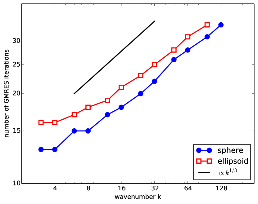
Figure 1: The number of iterations required for GMRES to converge (with tolerance $1\times 10^{-5}$) when GMRES is applied to the Galerkin matrix corresponding to the direct integral equation (1.2) with $\eta=k$, and with ${\Omega}$ the sphere or ellipsoid, and the values of $k$ from Tables 1 and 2. The $k^{1/3}$ rate is the upper bound on the rate guaranteed by Theorem 1.16.

We see from Figure 1 that the $k^{1/3}$ growth predicted by Theorem 1.16 appears to be effectively sharp. Indeed, the plot of the iterations for the ellipsoid becomes roughly linear from $k=12$ onwards, and estimating the slope of this line using the numbers of iterations at $k=12$ and $k=96$ we have that the $\#_{\text{iterations}}\sim k^{0.28}$. Using the numbers of iterations at $k=12$ and $k=96$ to estimate the rate of growth for the sphere we have that $\#_{\text{iterations}}\sim k^{0.29}$.

Finally, Table 3 compares the iteration counts and times for the sphere when $\eta=k$ and when $\eta=-k$. We see that, for every value of $k$ considered, the number of iterations when $\eta=-k$ is much greater than when $\eta=k$. Table 3 only goes up to $k=32$, since the $k=64$ run for the sphere with $\eta=-k$ did not complete.

	$\eta=k$
$k$	$\#_{\text{iterations}}$	time (s)
4	13	3.10
8	15	7.42
16	18	40.30
32	22	271.42

$\eta=-k$
$\#_{\text{iterations}}$	time (s)
44	3.46
88	9.04
405	75.38
11191	4502.05

Table 3: With ${\Omega}$ the sphere and $\eta=k$ or $\eta=-k$, the number of iterations required for GMRES to converge (with tolerance $1\times 10^{-5}$) and time taken to converge, when GMRES is applied to the Galerin matrix corresponding to the direct integral equation (1.2).

Remark 5.1 (The link between Table 3 and the recent work of Marburg [58, 59])

We performed the experiment in Table 3 because, in the engineering-acoustics literature, Marburg recently considered collocation discretisations of the direct integral equation for the Neumann problem (i.e. the Neumann-analogue of equation (1.2)) and showed that the analogue of the choice $\eta=k$ leads to much slower growth than the analogue of the choice $\eta=-k$ [58, 59].

A heuristic explanation for this dependence of the number of iterations on the sign of $\eta$ is essentially contained in the work of Levadoux and Michielsen [55, 56], and Antoine and Darbas [3]. In our setting of using the operator $A^{\prime}_{k,\eta}$ to solve the exterior Dirichlet problem, the key points are that

1. the ideal ${\rm i}\eta$ should approximate the Dirichlet-to-Neumann (DtN) map in ${\Omega_{+}}$, and

2. ${\rm i}k$ is a better approximation to the DtN map than $-{\rm i}k$ (at least for smooth convex obstacles).

Regarding 1: taking the Dirichlet trace of Green’s integral representation (written with general Dirichlet data, not just data coming from a plane wave as in (1.5)), and using the jump relations for the single- and double-layer potentials (see, e.g., [19, Equation 2.41]) we find that

$$\gamma^{+}u=-S_{k}(\partial_{n}^{+}u)+\left(\frac{1}{2}I+D_{k}\right)\gamma^{+}u.$$

Rearranging this equation, and introducing the notation $P_{\rm{DtN}}^{+}$ for the exterior Dirichlet-to-Neumann map for solutions of the Helmholtz equation in ${\Omega_{+}}$ satisfying the Sommerfeld radiation condition, we find that

$$I=\frac{1}{2}I+D_{k}-S_{k}P_{\rm{DtN}}^{+}.$$ (5.1)

Green’s second identity implies that, for $\phi,\psi\in H^{1/2}({\partial{\Omega}})$,

$$\langle P_{\rm{DtN}}^{+}\phi,\psi\rangle_{\partial{\Omega}}=\langle\phi,P_{\rm{DtN}}^{+}\psi\rangle_{\partial{\Omega}},$$

where the duality pairing $\langle\phi,\psi\rangle_{\partial{\Omega}}:=\int_{\partial{\Omega}}\phi\,\psi\,{\rm d}s$ when $\phi,\psi\in{L^{2}({\partial{\Omega}})}$; see [19, Equation 2.65, Equation 2.84, Equation A.24]. Therefore, taking the adjoint of (5.1), we find that

$$I=\frac{1}{2}I+D^{\prime}_{k}-P_{\rm{DtN}}^{+}S_{k}.$$ (5.2)

Comparing (5.2) to the definition of $A^{\prime}_{k,\eta}$ in (1.4), we see that the ideal ${\rm i}\eta$ should approximate $P_{\rm{DtN}}^{+}$. The idea of choosing $\eta$ as an operator, based on the relations (5.1)-(5.2) (and their analogues for the Neumann problem), essentially first appeared in [55], [56]. The relation (5.1) appeared explicitly in [3, Theorem 2.1], with this paper considering local approximations of the non-local operators $P_{\rm{DtN}}^{+}$ and $P_{\rm{NtD}}^{+}$, whilst [55], [56] used non-local pseudodifferential-operator approximations.

Regarding 2: In the case when $\partial\Omega$ is a circle (of radius $1$), the DtN map is given by

$$\frac{\partial u}{\partial r}(1,\theta)=k\sum_{n=-\infty}^{\infty}\frac{H_{n}^{(1)^{\prime}}(k)}{H_{n}^{(1)}(k)}{\rm e}^{{\rm i}n\theta}\,\left(\frac{1}{2\pi}\int^{2\pi}_{0}{\rm e}^{-{\rm i}n\phi}\,u(1,\phi)\,{\rm d}\phi\right).$$

The uniform- and double-asymptotic expansions of the Hankel functions (see, e.g., [67, §10.20, 10.41(v)]) imply that

$$k\frac{H_{n}^{(1)^{\prime}}(k)}{H_{n}^{(1)}(k)}\sim\begin{cases}{\rm i}k,&\text{ for }n\text{ fixed as }k\rightarrow\infty,\\ {\rm i}k\sqrt{1-\left(\frac{n}{k}\right)^{2}},&\,\,n,k\rightarrow\infty\text{ with }k-|n|\gg k^{1/3},\\ {\rm e}^{2\pi{\rm i}/3}\sqrt{\frac{n^{2}-k^{2}}{n^{2/3}\zeta}}\frac{{\rm Ai}^{\prime}\big{(}{\rm e}^{2\pi{\rm i}/3}n^{2/3}\zeta\big{)}}{{\rm Ai}\big{(}{\rm e}^{2\pi{\rm i}/3}n^{2/3}\zeta\big{)}},&\,\,n,k\rightarrow\infty\text{ with }\big{|}|n|-k\big{|}\leq Mk^{1/3},\\ n\sqrt{1-\left(\frac{k}{n}\right)^{2}},&\,\,n,k\rightarrow\infty\text{ with }|n|-k\gg k^{1/3},\end{cases}$$ (5.3)

where $\zeta$ is defined in terms of $n$ and $k$ by [67, Equations 10.20.2 and 10.20.3] . We see that the approximation $kH_{n}^{(1)^{\prime}}(k)/H_{n}^{(1)}(k)\sim{\rm i}k$ describes the DtN map on the low frequency modes and, in particular, is much better than the approximation $kH_{n}^{(1)^{\prime}}(k)/H_{n}^{(1)}(k)\sim-{\rm i}k$. The asymptotics (5.3), however, show that neither the approximations ${\rm i}k$ or $-{\rm i}k$ are particularly good on the higher frequency modes. An almost-identical analysis is valid for the sphere, and more generally for a smooth convex curved obstacle, since the symbol of the DtN map for such domains is described by the asymptotics (5.3); see [37, §9, last formula on page 58].

Acknowledgements.

The authors thank Timo Betcke (University College London), Simon Chandler-Wilde (University of Reading), and Sébastien Loisel (Heriot-Watt University) for useful discussions. In particular, EAS’s understanding of the improvement on the Elman estimate in [12] was greatly improved after seeing the alternative derivation of this result in [46, Equations 3.2 and 4.8]. This research made use of the Balena High Performance Computing (HPC) Service at the University of Bath. JG thanks the US National Science Foundation for support under the Mathematical Sciences Postdoctoral Research Fellowship DMS-1502661, and EAS thanks the UK Engineering and Physical Sciences Research Council for support under Grant EP/R005591/1.

References

- [1] F. Alouges, S. Borel, and D. P. Levadoux. A stable well-conditioned integral equation for electromagnetism scattering. Journal of computational and applied mathematics, 204(2):440–451, 2007.
- [2] A. Anand, Y. Boubendir, F. Ecevit, and F. Reitich. Analysis of multiple scattering iterations for high-frequency scattering problems. II: The three-dimensional scalar case. Numerische Mathematik, 114(3):373–427, 2010.
- [3] X. Antoine and M. Darbas. Alternative integral equations for the iterative solution of acoustic scattering problems. The Quarterly Journal of Mechanics and Applied Mathematics, 58(1):107–128, 2005.
- [4] X. Antoine and M. Darbas. Generalized combined field integral equations for the iterative solution of the three-dimensional Helmholtz equation. ESAIM: Mathematical Modelling and Numerical Analysis (M2AN), 41(1):147, 2007.
- [5] A. Asheim and D. Huybrechs. Extraction of uniformly accurate phase functions across smooth shadow boundaries in high frequency scattering problems. SIAM Journal on Applied Mathematics, 74(2):454–476, 2014.
- [6] K. E. Atkinson. The Numerical Solution of Integral Equations of the Second Kind. Cambridge Monographs on Applied and Computational Mathematics, 1997.
- [7] I. M. Babuška and S. A. Sauter. Is the pollution effect of the FEM avoidable for the Helmholtz equation considering high wave numbers? SIAM Review, pages 451–484, 2000.
- [8] L. Banjai and S. Sauter. A refined Galerkin error and stability analysis for highly indefinite variational problems. SIAM Journal on Numerical Analysis, 45(1):37–53, 2007.
- [9] D. Baskin, E. A. Spence, and J. Wunsch. Sharp high-frequency estimates for the Helmholtz equation and applications to boundary integral equations. SIAM Journal on Mathematical Analysis, 48(1):229–267, 2016.
- [10] S. K. Baydoun and S. Marburg. Quantification of numerical damping in the acoustic boundary element method for the example of a traveling wave in a duct. The Journal of the Acoustical Society of America, 141(5):3976–3976, 2017.
- [11] S. K. Baydoun and S. Marburg. Quantification of numerical damping in the acoustic boundary element method for two-dimensional duct problems. Journal of Theoretical and Computational Acoustics, page 1850022, 2018.
- [12] B. Beckermann, S. A. Goreinov, and E. E. Tyrtyshnikov. Some remarks on the Elman estimate for GMRES. SIAM journal on Matrix Analysis and Applications, 27(3):772–778, 2006.
- [13] T. Betcke, J. Phillips, and E. A. Spence. Spectral decompositions and non-normality of boundary integral operators in acoustic scattering. IMA J. Num. Anal., 34(2):700–731, 2014.
- [14] T. Betcke and E. A. Spence. Numerical estimation of coercivity constants for boundary integral operators in acoustic scattering. SIAM Journal on Numerical Analysis, 49(4):1572–1601, 2011.
- [15] Y. Boubendir, O. Bruno, D. Levadoux, and C. Turc. Integral equations requiring small numbers of Krylov-subspace iterations for two-dimensional smooth penetrable scattering problems. Applied Numerical Mathematics, 95:82–98, 2015.
- [16] O. Bruno, T. Elling, R. Paffenroth, and C. Turc. Electromagnetic integral equations requiring small numbers of Krylov-subspace iterations. Journal of Computational Physics, 228(17):6169–6183, 2009.
- [17] N. Burq, P. Gérard, and N. Tzvetkov. Restrictions of the Laplace-Beltrami eigenfunctions to submanifolds. Duke Math. J., 138(3):445–486, 2007.
- [18] S. N. Chandler-Wilde, I. G. Graham, S. Langdon, and M. Lindner. Condition number estimates for combined potential boundary integral operators in acoustic scattering. Journal of Integral Equations and Applications, 21(2):229–279, 2009.
- [19] S. N. Chandler-Wilde, I. G. Graham, S. Langdon, and E. A. Spence. Numerical-asymptotic boundary integral methods in high-frequency acoustic scattering. Acta Numerica, 21(1):89–305, 2012.
- [20] S. N. Chandler-Wilde, D. P. Hewett, S. Langdon, and A. Twigger. A high frequency boundary element method for scattering by a class of nonconvex obstacles. Numerische Mathematik, 129(4):647–689, 2015.
- [21] S. N. Chandler-Wilde and S. Langdon. A Galerkin boundary element method for high frequency scattering by convex polygons. SIAM Journal on Numerical Analysis, 45(2):610–640, 2007.
- [22] S. N. Chandler-Wilde and P. Monk. Wave-number-explicit bounds in time-harmonic scattering. SIAM Journal on Mathematical Analysis, 39(5):1428–1455, 2008.
- [23] S. N. Chandler-Wilde, M. Rahman, and C. R. Ross. A fast two-grid and finite section method for a class of integral equations on the real line with application to an acoustic scattering problem in the half-plane. Numer. Math., 93:1–51, 2002.
- [24] S. N. Chandler-Wilde, E. A. Spence, A. Gibbs, and V. P. Smyshlyaev. High-frequency bounds for the Helmholtz equation under parabolic trapping and applications in numerical analysis. arXiv preprint arXiv:1708.08415, 2017.
- [25] F. Chazal and R. Soufflet. Stability and finiteness properties of medial axis and skeleton. Journal of Dynamical and Control Systems, 10(2):149–170, 2004.
- [26] H. Christianson, A. Hassell, and J. A. Toth. Exterior Mass Estimates and -Restriction Bounds for Neumann Data Along Hypersurfaces. International Mathematics Research Notices, 6:1638–1665, 2015.
- [27] D. Colton and R. Kress. Inverse Acoustic and Electromagnetic Scattering Theory. Springer, 1998.
- [28] G. C. Diwan, A. Moiola, and E. A. Spence. Can coercive formulations lead to fast and accurate solution of the Helmholtz equation? Journal of Computational and Applied Mathematics, 352:110–131, 2019.
- [29] V. Domínguez, I. G. Graham, and V. P. Smyshlyaev. A hybrid numerical-asymptotic boundary integral method for high-frequency acoustic scattering. Numerische Mathematik, 106(3):471–510, 2007.
- [30] F. Ecevit. Frequency independent solvability of surface scattering problems. Turkish Journal of Mathematics, 42(2):407–417, 2018.
- [31] F. Ecevit and H. H. Eruslu. A Galerkin BEM for high-frequency scattering problems based on frequency-dependent changes of variables. IMA Journal on Numerical Analysis, to appear, 2018.
- [32] F. Ecevit and H. Ç. Özen. Frequency-adapted galerkin boundary element methods for convex scattering problems. Numerische Mathematik, 135(1):27–71, 2017.
- [33] F. Ecevit and F. Reitich. Analysis of multiple scattering iterations for high-frequency scattering problems. Part I: the two-dimensional case. Numerische Mathematik, 114:271–354, 2009.
- [34] S. C. Eisenstat, H. C. Elman, and M. H. Schultz. Variational iterative methods for nonsymmetric systems of linear equations. SIAM Journal on Numerical Analysis, pages 345–357, 1983.
- [35] H. C. Elman. Iterative Methods for Sparse Nonsymmetric Systems of Linear Equations. PhD thesis, Yale University, 1982.
- [36] J. Galkowski. Distribution of resonances in scattering by thin barriers. arXiv preprint arXiv:1404.3709 (to appear in Memoirs of the AMS), 2014.
- [37] J. Galkowski. The Quantum Sabine Law for Resonances in Transmission Problems. Pure and Applied Analysis, 1(1):27–100, 2019.
- [38] J. Galkowski and H. F. Smith. Restriction bounds for the free resolvent and resonances in lossy scattering. International Mathematics Research Notices, 16:7473–7509, 2015.
- [39] J. Galkowski and E. A. Spence. Wavenumber-explicit regularity estimates on the acoustic single- and double-layer operators. Integral Equations and Operator Theory, 91(6), 2019.
- [40] M. J. Gander, I. G. Graham, and E. A. Spence. Applying GMRES to the Helmholtz equation with shifted Laplacian preconditioning: What is the largest shift for which wavenumber-independent convergence is guaranteed? Numerische Mathematik, 131(3):567–614, 2015.
- [41] M. Ganesh and S. Hawkins. A fully discrete Galerkin method for high frequency exterior acoustic scattering in three dimensions. Journal of Computational Physics, 230:104–125, 2011.
- [42] M. Ganesh and C. Morgenstern. A sign-definite preconditioned high-order FEM. Part 1: Formulation and simulation for bounded homogeneous media wave propagation. SIAM J. Sci. Comp., 39(5):S563–S586, 2017.
- [43] M. Ganesh and C. Morgenstern. A sign-definite preconditioned high-order FEM Part-II: Formulation, Analysis, and simulation for bounded heterogeneous media wave propagation. preprint, 2017.
- [44] I. G. Graham, M. Löhndorf, J. M. Melenk, and E. A. Spence. When is the error in the -BEM for solving the Helmholtz equation bounded independently of ? BIT Numer. Math., 55(1):171–214, 2015.
- [45] A. Greenbaum. Iterative methods for solving linear systems. SIAM, 1997.
- [46] N. Greer and S. Loisel. The optimised Schwarz method and the two-Lagrange multiplier method for heterogeneous problems in general domains with two general subdomains. Numerical Algorithms, 69(4):737–762, 2015.
- [47] X. Han and M. Tacy. Sharp norm estimates of layer potentials and operators at high frequency. Journal of Functional Analysis, 269(9):2890–2926, 2015. with an appendix by J. Galkowski.
- [48] A. Hassell and M. Tacy. Semiclassical estimates of quasimodes on curved hypersurfaces. J. Geom. Anal., 22(1):74–89, 2012.
- [49] D. P. Hewett. Shadow boundary effects in hybrid numerical-asymptotic methods for high-frequency scattering. European Journal of Applied Mathematics, 26(05):773–793, 2015.
- [50] D. P. Hewett, S. Langdon, and S. N. Chandler-Wilde. A frequency-independent boundary element method for scattering by two-dimensional screens and apertures. IMA Journal of Numerical Analysis, 35(4):1698–1728, 2014.
- [51] D. P. Hewett, S. Langdon, and J. M. Melenk. A high frequency hp boundary element method for scattering by convex polygons. SIAM Journal on Numerical Analysis, 51(1):629–653, 2013.
- [52] F. Ihlenburg. Finite element analysis of acoustic scattering. Springer Verlag, 1998.
- [53] M. Ikawa. Decay of solutions of the wave equation in the exterior of several convex bodies. Ann. Inst. Fourier, 38(2):113–146, 1988.
- [54] A. Kirsch. Surface gradients and continuity properties for some integral operators in classical scattering theory. Mathematical Methods in the Applied Sciences, 11(6):789–804, 1989.
- [55] D. P. Levadoux. Etude d’une équation intégrale adaptée à la résolution hautes fréquences de l’équation d’Helmholtz. PhD thesis, Université Paris VI, 2001.
- [56] D. P. Levadoux and B. L. Michielsen. Nouvelles formulations intégrales pour les problèmes de diffraction d’ondes. ESAIM: Mathematical Modelling and Numerical Analysis, 38(01):157–175, 2004.
- [57] M. Löhndorf and J. M. Melenk. Wavenumber-Explicit -BEM for High Frequency Scattering. SIAM Journal on Numerical Analysis, 49(6):2340–2363, 2011.
- [58] S. Marburg. A review of the coupling parameter of the Burton and Miller boundary element method. Inter-noise and noise-con congress and conference proceedings, 249(2):4801–4806, 2014.
- [59] S. Marburg. The Burton and Miller method: Unlocking another mystery of its coupling parameter. Journal of Computational Acoustics, page 1550016, 2015.
- [60] S. Marburg. Numerical damping in the acoustic boundary element method. Acta Acustica united with Acustica, 102(3):415–418, 2016.
- [61] S. Marburg. Benchmark problem identifying a pollution effect in boundary element method. The Journal of the Acoustical Society of America, 141(5):3975–3975, 2017.
- [62] J. M. Melenk. Mapping properties of combined field Helmholtz boundary integral operators. SIAM Journal on Mathematical Analysis, 44(4):2599–2636, 2012.
- [63] R. B. Melrose and J. Sjöstrand. Singularities of boundary value problems. II. Comm. Pure Appl. Math., 35(2):129–168, 1982.
- [64] R. B. Melrose and M. E. Taylor. Near peak scattering and the corrected Kirchhoff approximation for a convex obstacle. Advances in Mathematics, 55(3):242 – 315, 1985.
- [65] A. Moiola and E. A. Spence. Is the Helmholtz equation really sign-indefinite? SIAM Review, 56(2):274–312, 2014.
- [66] C. S. Morawetz. Decay for solutions of the exterior problem for the wave equation. Communications on Pure and Applied Mathematics, 28(2):229–264, 1975.
- [67] NIST. Digital Library of Mathematical Functions. http://dlmf.nist.gov/, 2018.
- [68] Y. Saad. Iterative Methods for Sparse Linear Systems. SIAM, Philadelphia, 2003.
- [69] Y. Saad and M. H. Schultz. GMRES: A generalized minimal residual algorithm for solving nonsymmetric linear systems. SIAM Journal on Scientific and Statistical Computing, 7(3):856–869, 1986.
- [70] S. A. Sauter and C. Schwab. Boundary Element Methods. Springer-Verlag, Berlin, 2011.
- [71] V. Simoncini and D. B. Szyld. Recent computational developments in Krylov subspace methods for linear systems. Numerical Linear Algebra with Applications, 14(1):1–59, 2007.
- [72] W. Śmigaj, T. Betcke, S. Arridge, J. Phillips, and M. Schweiger. Solving Boundary Integral Problems with BEM++. ACM Trans. Math. Softw., 41(2):6:1–6:40, February 2015.
- [73] E. A. Spence. Wavenumber-explicit bounds in time-harmonic acoustic scattering. SIAM J. Math. Anal., 46(4):2987–3024, 2014.
- [74] E. A. Spence, S. N. Chandler-Wilde, I. G. Graham, and V. P. Smyshlyaev. A new frequency-uniform coercive boundary integral equation for acoustic scattering. Communications on Pure and Applied Mathematics, 64(10):1384–1415, 2011.
- [75] E. A. Spence, I. V Kamotski, and V. P Smyshlyaev. Coercivity of combined boundary integral equations in high-frequency scattering. Communications on Pure and Applied Mathematics, 68(9):1587–1639, 2015.
- [76] O. Steinbach. Numerical Approximation Methods for Elliptic Boundary Value Problems: Finite and Boundary Elements. Springer, New York, 2008.
- [77] M. Tacy. Semiclassical estimates of quasimodes on submanifolds. Comm. Partial Differential Equations, 35(8):1538–1562, 2010.
- [78] M Tacy. Semiclassical estimates for restrictions of the quantisation of normal velocity to interior hypersurfaces. arXiv preprint, arxiv : 1403.6575, 2014.
- [79] D. Tataru. On the regularity of boundary traces for the wave equation. Ann. Scuola Norm. Sup. Pisa Cl. Sci. (4), 26(1):185–206, 1998.
- [80] B. R. Vainberg. On the short wave asymptotic behaviour of solutions of stationary problems and the asymptotic behaviour as of solutions of non-stationary problems. Russian Mathematical Surveys, 30(2):1–58, 1975.
- [81] F. Vico, L. Greengard, and Z. Gimbutas. Boundary integral equation analysis on the sphere. Numerische Mathematik, 128(3):463–487, 2014.