Collective modes of trapped spinor Bose condensates

Abstract

We study the richer structures of quasi-one-dimensional Bogoliubov-de Genes collective excitations of $F=1$ spinor Bose-Einstein condensate in a harmonic trap potential loaded in an optical lattice. Employing a perturbative method we report general analytical expressions for the confined collective polar and ferromagnetic Goldstone modes. In both cases the excited eigenfrequencies are given as function of the 1D effective coupling constants, trap frequency and optical lattice parameters. It is shown that the main contribution of the optical lattice laser intensity is to shift the confined phonon frequencies. Moreover, for high intensities, the excitation spectrum becomes independent of the self-interaction parameters. We reveal some features of the evolution for the Goldstone modes as well as the condensate densities from the ferromagnetic to the polar phases.

I Introduction

Since the pioneering works of Ho PhysRevLett.81.742 and Ohmi and Machida, doi:10.1143/JPSJ.67.1822 a lot of effort have been devoted to study $F=1$ spinor Bose-Einstein condensates (BECs). Due to the internal degrees of freedom, the condensate presents a vectorial character and the wavefunction is described by three components in the hyperfine state with magnetic quantum number $m=$-1,0,1. Accordingly and depending of spin-exchange interaction values, PhysRevA.64.053602 ; PhysRevLett.88.093201 two phases are predicted: ferromagnetic (⁸⁷Rb) Chang2005 ; PhysRevLett.83.2498 ; PhysRevLett.87.010404 and polar or antiferromagnetic (²³Na). PhysRevLett.80.2027 ; PhysRevLett.82.2228 The experimental realization of spinor BECs, typically produced in optically trapped dilute gases, allows to study several interesting problems as magnetism, quantum phenomena not observed in single-component condensate,  Stenger1998 ; PhysRevLett.82.2228 spin dynamics, PhysRevLett.92.140403 the miscibility of the spinor components Stenger1998 as well as spin domains in an external magnetic field, and the nature of the ground state spinor condensates (see the recently overview in Ref. Kawaguchi2012253, and references there in).

An analysis of the collectives modes is an important step for a compressive study of the dynamics for both polar and ferromagnetic phases. Problems as quantized vortices, PhysRevLett.83.2498 superfluidity, spin-domains  Stenger1998 or damping processes, require an exhaustive knowledged of the dynamic process (see Refs.  PhysRevA.92.042502, ; PhysRevA.88.063638, ; PhysRevA.70.023611, ; PhysRevA.77.033610, ; 1367-2630-11-12-123012, ). Information of the collective excitations on the atom-atom self-interaction terms and on the applied external potential are fundamental bricks to build the dynamics of the phenomena above mentioned. The nature and evaluation of the Goldstone modes, so far, has been tackled assuming a spatial homogeneous Bose-Einstein condensate. PhysRevLett.81.742 ; doi:10.1143/JPSJ.67.1822 ; PhysRevLett.110.235302 ; Kawaguchi2012253 Thus, due to the concomitant translational symmetry the wavevector $\mathbf{k}$ is a good quantum number with Bogoliubov typical excitation $\omega=\omega(\mathbf{k}).$ However, this approach is not longer valid when the condensate is loaded into a confined spatial trap potential, in particular, the collective excitations must show a discrete set of modes or confined states.

In the present contribution we focus on the behavior of the Goldstone modes for $F=1$ spinor BECs confined in a cigar-shape geometry. The experimental realizations of two- and one-dimensional condensates in diluted ultracold atoms employing optical and magnetic traps are very well established technics. PhysRevLett.87.130402 ; PhysRevLett.87.160405 ; Science293 In general, however, the three dimensional nonlinear Gross-Pitaevskii equation (GPE) cannot be decoupled into transversal and longitudinal motions. Nevertheless, in presence of highly anisotropic trap potential, we can handled the problem as being tightly confined in a plane and with an independent 1D motion. Petrov Ref. PhysRevLett.81.742, shows that the three-dimensional ground state $\Psi_{m}$ of the alkali atoms of the condensate in the hyperfine state $\left|m\right\rangle$ $(m=-1,0,1)$ is ruled by

$$i\hslash\frac{\partial\Psi_{m}(x,\mathbf{r},t)}{\partial t}=\left[\frac{p^{2}}{2M}+U_{3D}+\right.\\ \left.\overline{c_{0}}\Psi_{a}^{\dagger}\Psi_{a}\right]\Psi_{m}(x,\mathbf{r},t)+\overline{c_{2}}\Psi_{a}^{{\dagger}}\mathbf{F}_{ab}\Psi_{b}\cdot\left[\mathbf{F}\Psi(x,\mathbf{r},t)\right]_{m}\text{ },$$ (1)

with $M$ being the mass of the atom, $\mathbf{F}$ the total hyperfine spin operator, $\overline{c_{0}}=(g_{0}+2g_{2})/3$, $\overline{c_{2}}=(g_{2}-g_{0})/3$, $g_{j}$ ($j=0,2$) the atom-atom self-interaction terms related to the s-wave scattering length, $a_{F}$ in the total spin $F$ channel and, additionally, depending on the total number of particles $N$. The order parameter can be written explicitly as $\Psi_{a}(x,\mathbf{r},t)=$ $\left|\Psi(x,\mathbf{r},t)\right|\zeta_{a}$, where $\zeta_{a}$ is the normalized spinor state and $\int_{{\mathbb{R}}}\left|\Psi_{a}(x,\mathbf{r},t)\right|^{2}\,dxd\mathbf{r}=1.$ Above, we have written $(x,\mathbf{r})$ as the 3D spatial vector position, with $x$ being the longitudinal coordinate and $\mathbf{r}$ the 2D transverse vector.

In Eq. (1) we consider a condensate confined in anisotropic harmonic trapping potential and loaded into an optical lattice as given by the external potential

$$U_{3D}(x,\mathbf{r})=\frac{1}{2}M\left(\omega_{0}^{2}x^{2}+\omega_{\mathbf{r}}^{2}\mathbf{r}^{2}\right)-V_{L}\cos^{2}(\frac{2\pi}{d}x)\text{ },$$ (2)

where $\omega_{0}$ and $\omega_{\mathbf{r}}$ are the longitudinal and transversal harmonic oscillator frequencies, respectively, $V_{L}$ is proportional to the laser intensity and $d$ the laser wavelength. Assuming now that the longitudinal motion is adiabatic with respect to the transverse one, and considering a highly anisotropic harmonic trapping, with $\omega_{0}$ $\ll$ $\omega_{\mathbf{r}}$, the 3D order parameter can be factorized into PhysRevA.74.023607 $\Psi_{m}(x,\mathbf{r},t)=\phi_{m}(x;t)\chi(x,\mathbf{r})$. We note two important consequences of these assumptions, one, the transverse motion is independent of the hyperfine state $\left|m\right\rangle$ and, second, all the time evolution occurs along the 1D longitudinal coordinate $x$. It then follows from Eqs. ( 1) and (2) that the motion in the plane is given by the equation PhysRevLett.89.110401 ; refId0

$$\left[\frac{p_{\mathbf{r}}^{2}}{2M}+\frac{M}{2}\omega_{\mathbf{r}}^{2}\mathbf{r}^{2}+\left(\overline{c_{0}}\left|\phi_{a}\right|^{2}+\frac{1}{\phi_{m}}\overline{c_{2}}\phi_{a}^{{\dagger}}\mathbf{F}_{ab}\phi_{b}\cdot\left(\mathbf{F}\phi\right)_{m}\right)\times\right.\\ \left.\left|\chi(x,\mathbf{r})\right|^{2}\right]\chi=\mu_{\mathbf{r}}\left[\phi_{m}\right]\chi\text{ },$$ (3)

where the transverse chemical potential, $\mu_{\mathbf{r}}\left[\phi_{m}\right]$, is a functional of the 1D order parameter $\phi_{m}(x;t)$. For the longitudinal dynamic part we have

$$i\hslash\frac{\partial\phi_{m}(x;t)}{\partial t}=\left[\frac{p_{x}^{2}}{2M}+\frac{M}{2}\omega_{0}^{2}x^{2}-\right.\\ \left.V_{L}\cos^{2}(\frac{2\pi}{d}x)+\mu_{\mathbf{r}}\left[\phi_{m}\right]\right]\phi_{m}(x;t)\text{ }.$$ (4)

In a first approach the function $\chi(x,r)$ can be described by the ground state of a 2D harmonic oscillator with frequency $\omega_{\mathbf{r}}$. Thus, expanding $\mu_{\mathbf{r}}$ as a Taylor series of the wavefunction $\phi_{m}$ and following the same trend as giving in Refs.  refId0, and carretero, we have

$$\mu_{\mathbf{r}}\left[\phi_{m}\right]\phi_{m}\approx\hslash\omega_{\mathbf{r}}\phi_{m}+C_{m}\phi_{m}+.....\text{ },$$ (5)

with $C_{m}\phi_{m}=c_{0}\left|\phi_{m}\right|^{2}\phi_{m}+c_{2}\phi_{a}^{{\dagger}}\mathbf{F}_{ab}\phi_{b}\cdot\left(\mathbf{F}\phi\right)_{m}$, $c_{0}=M\omega_{\mathbf{r}}\overline{c_{0}}/(3\hslash\pi)$ and $c_{2}=M\omega_{\mathbf{r}}\overline{c_{2}}/(3\hslash\pi)$ becoming the effective self-interaction constants for the 1D cigar-shape spinor BEC. Hence, Eq. (4) is reduced to

$$i\hslash\frac{\partial\phi_{m}(x;t)}{\partial t}=\left[\frac{p_{x}^{2}}{2M}+\frac{M}{2}\omega_{0}^{2}x^{2}-V_{L}\cos^{2}(\frac{2\pi}{d}x)+\right.\\ \left.c_{0}\left|\phi_{m}\right|^{2}\right]\phi_{m}(x;t)+c_{2}\phi_{a}^{{\dagger}}\mathbf{F}_{ab}\phi_{b}\cdot\left(\mathbf{F}\phi\right)_{m}\text{ }.$$ (6)

Starting now from the 1D spinor GPE, Eq. (6), the main contribution of this work is the description of the collective longitudinal modes, providing explicit expressions for the corresponding excited wavefunctions, $\varphi_{m,k}(x;t)$, and their eigenfrequencies, $\hslash\omega_{m}^{(k)}$ ($k=1,2,\dots$). In Sec. II we consider the quasi-1D generalized Bogoliubov-deGennes equations (B-dGEs), which allows for the analysis of the polar and ferromagnetic phases and the interplay between the non-linear terms, on one hand, and the harmonic trapping, and the optical lattice external potentials on the other one. As we stated above, the system is consider as spatially inhomogeneous and in consequence we are in presence of confined Goldstone modes or confined phonon like spectrum. Section III is devoted to the excitation amplitudes for both phases considered, and our conclusions are listed in Sec. IV. The main elements for the description of the eigenfrequencies and eigenfunctions are summarized in the Appendixes A and B, respectively.

II Excited states

Using Bogoliubov approximation at very low temperature, Pitaevskii the collective excitation states of the generalized 1D GPE (6) can be represented by the wavefunction having the form

$$\varphi_{m,k}(x;t)=\text{exp}(-i\mu t/\hbar)\left[\phi_{0}(x)\right.\\ \left.+\varphi_{m}^{(k)}\text{exp}(-i\omega_{m}^{(k)}t)+\varphi_{\mp m}^{{\dagger}(k)}\text{exp}(i\omega_{m}^{(k)}t)\right]\text{,}$$ (7)

where $\varphi_{m}^{(k)}$ represents a small fluctuation from the stationary solutions $\phi_{0}(x)\text{exp}(-i\mu t/\hbar)$ with the sign ( $\mp)$ for the polar ($P$) and the ferromagnetic ($Fe)$ phases, respectively and $\mu$ the 1D chemical potential. Following Eq. (7), the wavefunctions of the collective modes for the condensate satisfy the generalized 1D B-dGEs Pitaevskii ; PhysRevLett.81.742

$$i\hbar\frac{\partial}{\partial t}\left(\begin{array}[]{c}\varphi_{m}^{(k)}\\ -\varphi_{\mp m}^{{\dagger}(k)}\end{array}\right)=\left(\begin{array}[]{cc}L_{0}&\overline{\lambda_{m}^{(J)}}|\phi_{0}|^{2}\\ \overline{\lambda_{m}^{(J)}}|\phi_{0}|^{2}&L_{0}\end{array}\right)\left(\begin{array}[]{c}\varphi_{m}^{(k)}\\ \varphi\varphi_{\mp m}^{{\dagger}(k)}\end{array}\right)\text{ },$$ (8)

where $J$ =($P$, $Fe$) and the operator $L_{0}$ is defined as

$$L_{0}=\frac{1}{2M}p_{x}^{2}+U-\mu+\lambda_{m}^{(J)}|\phi_{0}|^{2}\text{ }.$$ (9)

In Eq. 8) and (LABEL:L0), the coupling parameters are given by,

$$\lambda_{m}^{(P)}=\left\{\begin{array}[]{cc}2c_{0};&m=0\\ g_{2};&m=\pm 1\end{array}\right.\text{, \ \ }\overline{\lambda_{m}^{(P)}}=\left\{\begin{array}[]{cc}c_{0};&m=0\\ c_{2};&m=\pm 1\end{array}\right.\text{ }.$$ (10)

and

$$\lambda_{m}^{(Fe)} = \left\{\begin{array}[]{cc}g_{2};&m=0\\ g_{2}+2\left|c_{2}\right|;&m=-1\\ 2g_{2};&m=1\end{array}\right.\text{ ,}$$ (14)

$$\text{\ }\overline{\lambda_{m}^{(Fe)}} = \left\{\begin{array}[]{cc}0;&m=-1,0\\ g_{2};&m=1\end{array}\right.\text{ }.$$ (17)

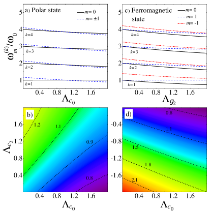
Figure 1: (Color online) Upper panel: Collective excitation frequencies $\omega_{m}^{(k)}$, in units of the trap frequency potential $\omega_{0}$, of the first four modes. a) $\omega_{P,m}^{(k)}$ as function of $\Lambda_{c_{0}}$; b) $\omega_{Fe,m}^{(k)}$ as function of $\Lambda_{g_{2}}$. Lower panel: Contour maps as function of 1D self-interaction constants $\Lambda_{c_{0}}$ and $\Lambda_{c_{2}}$: c) $\omega_{P,\pm 1}^{(1)}$; d) $\omega_{Fe,1}^{(1)}$. In the calculation $V_{L}=0$.

The order parameter $\phi_{0}$ is described by the GPE

$$\left[\frac{1}{2M}p_{x}^{2}+U(x)+g_{1}|\phi_{0}|^{2}\right]\phi_{0}=\mu\phi_{0}\text{ },$$ (18)

with $U(x)=M\omega_{0}^{2}x^{2}/2-V_{L}\cos^{2}(2\pi x/d)$,

$$g_{1}=\left\{\begin{array}[]{ccc}c_{0}&\rightarrow&\text{polar state}\\ g_{2}&\rightarrow&\text{ferromagnetic state}\end{array}\right.\text{ .}$$

We search for the solution of Eq. (18) with the boundary conditions $\phi_{0}\rightarrow 0$ at $x\rightarrow\pm\infty$ and normalized to $\int|\phi_{0}(x)|^{2}dx=1.$ Analytical expressions for the order parameter, $\phi_{0},$ and the chemical potential, $\mu,$ solution of Eq. ( 18) for a given self-interaction constant $g_{1}$, are reported in Ref. PhysRevA.79.063621, .

II.1 Polar phase

II.1.1 Homogeneous System.

First, we consider a negligible intensity for the external trap potential and without an optical lattice, in which the system can be considered as homogeneous. In this situation, the density $n_{0}$ is constant within all space and the system presents spatial symmetry invariance. Hence, the linear momentum $p_{x}$ is a good quantum number. Solving the system of Eqs. (8), for the phonon-like Bogoliubov excitation spectrum in the low-momentum regime, we have that $\hslash\omega_{P,0}=\sqrt{\varepsilon_{p_{x}}(\varepsilon_{p_{x\text{ }}}+2c_{0}n_{0})}$ and $\hslash\omega_{P,\pm 1}=\sqrt{\varepsilon_{p_{x}}(\varepsilon_{p_{x}}+2c_{2}n_{0})}$ with $\varepsilon_{p_{x}}=p_{x}^{2}/2M$. Bogolyubov ; PhysRevLett.79.4056 ; Pitaevskii

II.1.2 Confined Phonons.

If we now tackled the problem with the external 1D trap potential $M\omega_{0}^{2}x^{2}/2\neq 0$, the spatial symmetry invariance is broken and we are facing to a discreet set of confined phonon-like modes with frequencies $\omega_{P,m}^{(k)}$ $(k=1,2,...)$. Equations (18) and (8) form an independent 3$\times$3 system of equations for $m=0$ and $\pm 1$. By considering both, the nonlinear terms $\overline{\lambda_{m}^{(P)}}|\phi_{0}|^{2}$ and the optical lattice potential in the B-dGEs (8) as a perturbation with respect to the harmonic trap, we are able to get the collective phonon mode frequencies, $\omega_{P,m}^{(k)}$, for each hyperfine state $\left|m\right\rangle$. A description of the employed perturbative algorithm is given elsewhere. EPJDTrallero2012 ; PhysRevA.92.042502 According to the values of the interaction constant $\lambda_{m}^{(P)}$, the inherent symmetry of the system (8) shows that the states with $m=\pm 1$ are degenerate. The corresponding analytical results for the eigenfrequencies $\omega_{P,m}^{(k)}$ are displayed in the Appendix A. In the upper panel of Fig. 1a) we show $\omega_{P,m}^{(k)}$ in units of $\omega_{0}$ for the first 4 modes and $m=0$, $\pm 1$ as a function of the dimensionless interaction parameter $\Lambda_{c_{0}}=c_{0}/(l_{0}\hbar\omega_{0})$ for the repulsive case $\Lambda_{c_{0}}>0$. Here $l_{0}=\sqrt{\hslash/(M\omega_{0})}$. We observe that $\omega_{P,0}^{(1)}=\omega_{0}$ is constant independent of the self-interaction constants, Pitaevskii while the other modes $\omega_{P,m}^{(k)}$ decreasing as $\Lambda_{c_{0}}$ increases. It is interesting to note that for $\Lambda_{c_{0}}>\Lambda_{c_{2}}=c_{2}/(l_{0}\hbar\omega_{0})$ the first excited state correspond to $\omega_{P,\pm 1}^{(1)}$ and in general $\omega_{P,\pm 1}^{(k)}>\omega_{P,0}^{(k)},$ $\forall$ $k$ (see Appendix A Eqs. (22) and (23)). In Fig. 1b) the evolution of the collective excitation $\omega_{P,\pm 1}^{(1)}$ is shown in terms of the interactions $\Lambda_{c_{0}}$ and $\Lambda_{c_{2}}$. For given values of the parameter $\Lambda_{c_{0}}$ we observe that the frequency increases monotonically as $\Lambda_{c_{2}}$ increases. In these calculations we fixed the intensity of the optical lattice as $V_{L}=0$.

II.2 Ferromagnetic phase

II.2.1 Homogeneous System

This phase emerges when $c_{2}<0$ and we have three set of non-degenerate states $\varphi_{m}^{(k)}(x)$ for $m=-1,0,1$. As in the Polar case, the energies of the excited states are obtained directly from the Eqs (18 ) and (8) and can be cast as $\hslash\omega_{Fe,-1}=\varepsilon_{p_{x}}+2c_{2}n_{0}$, $\hslash\omega_{Fe,0}=\varepsilon_{p_{x}}$, and $\hslash\omega_{Fe,1}=\sqrt{\varepsilon_{p_{x}}(\varepsilon_{p_{x}}+2g_{2}n_{0})}$. Here, the only phonon-like Bogoliubov spectrum corresponds to the state $\varphi_{1}(x)$ with frequency $\omega_{Fe,1}$.

II.2.2 Confined Phonons

In the present case, the system (8) is decoupled into two independent equations for $\varphi_{Fe,0}^{(k)}$ and $\varphi_{Fe,-1}^{(k)}$, and $3x3$ system of equations for the state with $m=1$. Following the same procedure mentioned above for the Polar phase, in Appendix A we report the analytical solutions for the three independent excited frequencies $\omega_{Fe,m}^{(k)}$, $m=-1,0,1$, $\forall$ $k$. Figures 1b) and d) are devoted to the collective excitations for the ferromagnetic phase. In the upper panel of the figure we observe the three independent set ($m=-1,0,1$) of confined frequencies ($k=1,2,3,4$) as a function of $\Lambda_{g_{2}}=g_{2}/(l_{0}\hbar\omega_{0})$. All frequencies decrease as $\Lambda_{g_{2}}$ increases, while the state $(m=1,k=1)$ is independent of the interaction constants.Notice that the states with $m=-1,0$ do not fulfill typical properties of B-dGE solutions, for instance, their first excited state is independent of the interaction. This appears to be in correspondence with the fact that in the homogeneous case, their dispersion relations are not linear in the low-momentum regime.. In 1d) the characteristic contour map for the reduced confined phonon frequency $\omega_{Fe,-1}^{(1)}/\omega_{0}$ is represented as a function of $\Lambda_{c_{0}}$ and $\Lambda_{c_{2}}$. For a given value of $\Lambda_{c_{0}}$ the frequency $\omega_{Fe,-1}^{(1)}$ decreases as $\Lambda_{c_{2}}\rightarrow 0$ in correspondence with the result shown in Fig. 2, as discussed below.

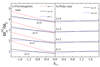
Figure 2: (Color online) Evolution of the frequencies modes ($k=1,2,3$, and 4 ) from the ferromagnetic phase to the polar phase as a function $\Lambda_{c_{2}}$. Left (right) panel $\Lambda_{g_{2}}=1$ ($\Lambda_{c_{0}}=1$).

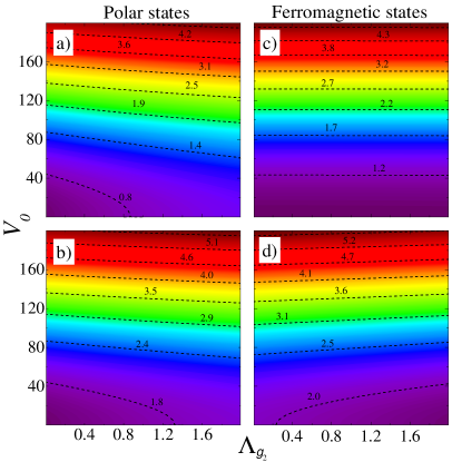
Figure 3: (Color online) Contour plot of the excited frequencies $\omega_{m}^{(k)}$ as function of dimensionless parameters $\Lambda_{g_{2}}$ and $V_{0}=V_{L}/\hslash\omega_{0}$ for the first two modes $k=1,2$ . Left panel: Polar state for $\omega_{\pm 1}^{(k)}$. Right panel: Ferromagnetic state and $\omega_{1}^{(k)}$.

The transition from the ferromagnetic to the polar phase is represented in Fig. 2 for the modes with frequencies $\omega_{m}^{(k)}$ ($k=1,2,3,4$) as function of $\Lambda_{c_{2}}$. In the panel a) of the figure for $\Lambda_{c_{2}}<0$, the three set of independent modes with $m=-1,0,-1$ are very well resolved. They show different behavior as $\Lambda_{c_{2}}$ decreases with the stronger slope for the phonon modes $\omega_{-1}^{(k)}$. For $\Lambda_{c_{2}}=0$, the states $m=-1,0$ become degenerate, while for $\Lambda_{c_{2}}$ positive, the values of $\omega_{P,m}^{(k)}$ are closer to $k\omega_{0}$, (see panel a)), i.e. the influence of $\Lambda_{c_{2}}$ is negligible and we have that these three states are quasi-degeneracy.

An important issue is the influence of the optical lattice on the collective excitations. Figure 3 shows contour plot of the frequencies $\omega_{m}^{(k)}$ for the first two states ($k=1,2$) as a function of the dimensionless laser intensity $V_{L}$ and the parameter $\Lambda_{c_{2}}$ for the polar state, $m=\pm 1$, and the ferromagnetic one, $m=1$. The main contribution of $V_{L}$ is to shift the confined phonon frequency. For larger values of $V_{L}$, the frequency is almost independent of $\Lambda_{c_{2}}$, while the mayor modification of $\omega_{m}^{(k)}$ occurs for lower values of laser intensity, $V_{L}\sim 40\hbar\omega_{0}$. These facts are explained by Eqs. (26) and (29) that take into account the interplay between the self-interaction constant $\Lambda_{c_{2}}$ and the presence of the optical lattice.

III Excitation amplitudes

The wavefunction of the excited states for the polar and ferromagnetic phase are displayed in the Appendix B. The calculation of $\varphi_{m}^{(k)}(x;t)=\varphi_{m}^{(k)}$exp$(-i\omega_{m}^{(k)}t)$ is obtained in first order of perturbation for the self-interaction constants $\Lambda_{c_{0}}$, $\Lambda_{c_{2}},$ $\Lambda_{g_{2}}$ and dimensionless laser intensity $V_{0}=V_{L}/\hslash\omega_{0}$. As it is states in the Appendix  B, the space of solutions $\varphi_{m}^{(k)}(x)$ is composed of two independent Hilbert subspaces $\mathcal{H}_{\mathcal{I}}$ and $\mathcal{H}_{\mathcal{II}}$ for odd ($k=1,3,...)$ and even ($k=2,4,$…) wavefunctions with respect to the inversion symmetry $x\rightarrow-x.$

The condensate density perturbation for a given phonon frequeny $\omega_{m}^{(k)}$ can be cast as

$$\delta\varphi_{m}^{(k)}=\frac{|\varphi_{m,k}(x;t)|^{2}-|\phi_{0}(x)|^{2}}{\sqrt{N}}\text{ }.$$ (19)

Thus, employing the results of the Appendix B for the wavefunction of the excited states of the polar state with $m=0$, we obtain an analytical representation for the function $\delta\varphi_{0}^{(k)}$, given by

$$\delta\varphi_{0}^{(k)}=2\text{cos}(\omega_{0}^{(k)}t)\left[\phi_{0}(x)\overline{\phi_{k}(x)}-\frac{\text{exp}(-x^{2})}{\sqrt{\pi^{\frac{1}{2}}}}\times\right.\\ \left(\Lambda_{c_{0}}\frac{f_{k,0}}{k\sqrt{\pi^{\frac{1}{2}}}}+\left\{\sum_{m\neq k}\Lambda_{c_{0}}\left(\frac{2}{k-m}-\frac{1}{k+m}\right)f_{k,m}\right.\right.\\ \left.\left.\left.-V_{0}\frac{g_{k,m}}{2(k-m)}\right\}\overline{\phi_{k}(x)}\right)\right]\text{ }.$$ (20)

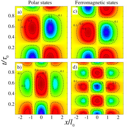
Figure 4: Contour map of the 1D condensate density perturbation, $\delta\varphi_{1}^{(k)}(x,t)$, for the first two excited state $(k=1,2)$. Left panel: Polar modes for $\Lambda_{c_{2}}=0.5$ and $\Lambda_{g_{2}}=2$. Right panel: Ferromagnetic modes for $\Lambda_{g_{2}}=1$. In the calculation $\tau_{0}=2\pi/\omega_{0}$ and $V_{L}=0$

Similar results can be obtained for the Bogoliubov-type excitation amplitudes listed in the Appendix B. In Fig. 4 it is shown a contour plot of the condensate density perturbation $\delta\varphi_{1}^{(k)}(x;t)$ for the polar and ferromagnetic phases. Here, we consider the first two excited states, the first one with $k=1$ belongs to the Hilbert subspaces $\mathcal{H}_{\mathcal{I}}$, while for $k=2$ to $\mathcal{H}_{\mathcal{II}}.$ The antisymmetric and symmetric character of $\delta\varphi_{1}^{(k)}$ for both phases, are clearly seen in the figure. In general, the evolution from one phase to another as a function of the parameter $\Lambda_{c_{2}}$ does not change the parity of a the density perturbation $\delta\varphi_{m}^{(k)}(x;t)$.

IV Conclusion

In conclusion, we have solved the multicomponent order parameter of the coupled Bogoliubov-de Genes equations, Eq. (8), for the one dimensional cigar-shaped Bose-Einstein condensates with $F=1$ spin degrees of freedom. We have presented useful analytical expressions for the confined phonon frequencies and wavefunctions of the excited states for the ferromagnetic and antiferromagnetic phases. The examen of the Goldstone modes shows that the phonon energies, in both polar and ferromagnetic phases, are proportional to the longitudinal harmonic trap frequency. We conclude that the phonon modes are weakly dependent on the interaction constants for the antiferromagnetic states, while a more pronounced structure is reached in the case of BEC loaded in the ferromagnetic phase (see Fig. (1) and (2)). Also, we found the existence of a set of the self-interaction constant values for which the lower frequency lies below of the harmonic oscillator frequency $\omega_{0}$ . The modes for the polar $m=0$ and ferromagnetic $\ m=-1$ states coincide with the oscillation of the center of mass and are independent of the atom-atom interactions. Pitaevskii In contrast to results obtained in the framework of Thomas-Fermi approximation, where the density of excited polar modes are interaction independent (see Refs.  PhysRevLett.81.742, and PhysRevLett.77.2360, ), we have found here that the condensate densities, $\delta\varphi_{m}^{(k)},$ show a clear structure and depend on the $g_{0}$ and $g_{2}$ atom-atom self-interaction terms.

Appendix A Exited frequencies

Introducing the dimensionless interaction self-interaction constant $\Lambda_{C}=C/(l_{0}\hbar\omega_{0})$ ($C=c_{0},c_{2}$, and $g_{2}$), $l_{0}=\sqrt{\hslash/(M\omega_{0})}$, $V_{0}=V_{L}/\hslash\omega_{0}$ and $\alpha=2\pi l_{0}/d$, the eigenfrequencies, $\omega_{m}^{(k)}$, of Eq. ( 8) are obtained in the framework of a perturbative regime where the non-linear terms $\Lambda_{C}\left|\phi_{m}\right|^{2}$ and the periodic potential $V_{0}\cos^{2}(\alpha x/l_{0})$ are considered as a perturbation with respect to the trap potential. We defined the auxiliary function

$$\frac{\omega^{(k)}(z1,z2,z3)}{\omega_{0}}=k-\frac{z_{1}}{\sqrt{2\pi}}+\frac{\Gamma(k+\frac{1}{2})}{\sqrt{2}\pi k!}z_{2}-\\ -\frac{V_{0}}{2}\text{exp}(-\alpha^{2})[L_{k}(2\alpha^{2})-1]-\frac{z_{1}V_{0}}{\sqrt{2\pi}}\text{exp}(-\alpha^{2})\left[Ei\text{(}\frac{\alpha^{2}}{2})\right.\\ \left.-\text{ln(}\frac{\alpha^{2}}{2})-\mathcal{C}\right]-\frac{z_{2}V_{0}}{\sqrt{2}\pi}\text{exp}(-\alpha^{2})\delta_{k}(\alpha)+\frac{V_{0}^{2}}{4}\text{exp}(-2\alpha^{2})\times\\ \left[Chi\text{(}2\alpha^{2})-ln\text{(}2\alpha^{2})-\mathcal{C}+\rho_{k}(\alpha)\right]+0.033106z_{1}^{2}+\\ \left(\gamma_{k}^{(1)}z_{3}^{2}+\frac{\gamma_{k}^{(2)}}{4}z_{2}^{2}\right)\frac{1}{2\pi^{2}}\text{ },$$ (21)

with $\Gamma(z)$ being the Gamma function, $L_{k}(z)$ the Laguerre polynomials, $\mathcal{C}$ the Euler’s constant $Ei(z)$ and $Chi(z)$ the exponential and cosine hyperbolic integrals, respectively, and  $k=1,2,....$ . Functions $\delta_{k}(\alpha)$ and $\rho_{k}(\alpha)$ are reported in Ref. (PhysRevA.92.042502, ) and the values of $\gamma_{k}^{(1)}$ and $\gamma_{k}^{(2)}$ for $k=1,2,...,6$ are listed in Table I.

Table 1: Values of the constants $\gamma_{k}^{(1)}$ and $\gamma_{k}^{(2)}$. They satisfice the equation $\gamma_{k}=\gamma_{k}^{(1)}+\gamma_{k}^{(2)}$ and $\gamma_{k}$ given in Ref. EPJDTrallero2012, .

$k$	1	2	3	4	5	6
$\gamma_{k}^{(1)}$	-0.284	-0.620	0.142	0.015	0.093	0.050
$\gamma_{k}^{(2)}$	-0.486	-0.165	-0.162	-0.095	-0.079	-0.058

Polar modes.

Using the definition (21), it is possible to show that the Polar phonon modes with $m=0$ are given by

$$\omega_{P,0}^{(k)}=\omega^{(k)}(\Lambda_{c_{0}},2\Lambda_{c_{0}},\Lambda_{c_{0}})\text{ .}$$ (22)

On the other hand for the phonon frequencies $\omega_{P,\pm 1}^{(k)}$ we have

$$\omega_{P\pm 1}^{(k)}=\omega^{(k)}(\Lambda_{c_{0}},\Lambda_{g_{2}},\Lambda_{c_{2}})\text{ }.$$ (23)

Ferromagnetic modes.

The confined phonon frequencies for the $m=0$ ferromagnetic states can be cast as

$$\omega_{Fe,0}^{(k)}=\omega^{(k)}(\Lambda_{g_{2}},\Lambda_{g_{2}},0)\text{ }.$$

The modes with $m=1$ have the eigenfrequencies

$$\omega_{Fe,1}^{(k)}=\omega^{(k)}(\Lambda_{g_{2}},2\Lambda_{g_{2}},\Lambda_{g_{2}})\text{ },$$

and for $m=-1$ we obtain

$$\omega_{Fe,-1}^{(k)}=\omega^{(k)}(\Lambda_{g_{2}},\Lambda_{g_{2}}+2\left|\Lambda_{c_{2}}\right|,0)\text{ }.$$

Appendix B Wavefunction of the excited states

In first order of perturbation $\Lambda_{g_{2}}$ and $V_{0}$ we obtain the eigensolutions $\varphi_{m}^{(k)}$. Firstly, we introduce the auxiliary function

$$\digamma_{m}^{(k)}(y,t;z_{1},z_{2})=\overline{\phi_{k}(y)}\exp(-i\omega_{m}^{(k)}t)+\\ \sum_{p\neq k}\left[\frac{4z_{1}f_{k,p}(y)-V_{0}g_{k,p}(y)}{2(k-p)}\right.\\ \left.\overline{\phi_{p}(z)}\exp(-i\omega_{m}^{(k)}t)\right]-\\ \sum_{p=0}^{\infty}\frac{z_{2}f_{k,p}(y)}{k+p}\overline{\phi_{p}(y)}\exp(i\omega_{m}^{(k)}t)\text{ ,}$$ (24)

where $y=x/l_{0}$, $\overline{\phi_{p}(y)}$ are the 1D harmonic oscillator wavefunctions and the functions $f_{k,p}(y),$ $g_{k,p}(y)$ are given elsewhere. PhysRevA.79.063621 In Eq. (24) for a given state $\left|m\right\rangle$, the matrix elements $f_{k,p}(y)$ and $g_{k,p}(y)$ must fulfill the parity condition $k+p=$ even number. Thus, if $k$ is odd $\digamma_{m}^{(k)}$ is antisymmetric, while for $k$ even the function (24) is symmetric. In consequence, the density perturbation $\delta\varphi_{m}^{(k)}$ is restricted by the symmetry property of the $\digamma_{m}^{(k)}$ function.

For the polar state the excited wavefunction with $m=0$ is reduced to

$$\varphi_{P;k,m=0}=\exp(-i\mu t/\hslash)\left[\phi_{0}(y)+\digamma_{0}^{(k)}(y,t;\Lambda_{c_{0}},\Lambda_{c_{0}})\right]\text{ ,}$$ (25)

while for the case of $m\pm 1$ we obtain

$$\varphi_{P;k,m=\pm 1}=\exp(-i\mu t/\hslash)\left[\phi_{0}(y)+\right.\\ \left.\digamma_{\pm 1}^{(k)}(y,t;\Lambda_{g_{2}}/2,\Lambda_{c_{2}})\right]\text{ .}$$ (26)

For the ferromagnetic phase, the excited states are described by

$$\varphi_{Fe;k,m=-1}=\exp(-i\mu t/\hslash)\left[\phi_{0}(y)+\right.\\ \left.\digamma_{-1}^{(k)}(y,t;\Lambda_{g_{2}}+2|\Lambda_{c_{2}}|,0)\right]\text{ ,}$$ (27)

$$\varphi_{Fe;k,m=0}=\exp(-i\mu t/\hslash)\left[\phi_{0}(y)+\right.\\ \left.\digamma_{0}^{(k)}(y,t;\Lambda_{g_{2}}/2,0)\right]\text{ ,}$$ (28)

$$\varphi_{Fe;k,m=1}=\exp(-i\mu t/\hslash)\left[\phi_{0}(y)+\right.\\ \left.\digamma_{1}^{(k)}(y,t;\Lambda_{g_{2}},\Lambda_{g_{2}})\right]\text{ .}$$ (29)

References

• (1) T.-L. Ho, Phys. Rev. Lett., 81, 742 (1998).
• (2) T. Ohmi and K. Machida, Journal of the Physical Society of Japan, 67, 1822 (1998).
• (3) N. N. Klausen, J. L. Bohn, and Ch. H. Greene, Phys. Rev. A, 64, 053602 (2001).
• (4) E. G. M. van Kempen, S. J. J. M. F. Kokkelmans, D. J. Heinzen, and B. J. Verhaar, Phys. Rev. Lett., 88, 093201 (2002).
• (5) M. R. Matthews, B. P. Anderson, P. C. Haljan, D. S. Hall, C. E. Wieman, and E. A. Cornell,Phys. Rev. Lett., 83, 2498 (1999).
• (6) M. D. Barrett, J. A. Sauer, and M. S. Chapman, Phys. Rev. Lett., 87, 010404 (2001).
• (7) M.-S. Chang, Q. Qin, W. Zhang, L. You, and M. S. Chapman, Nat Phys, 1, 111 (2005).
• (8) D. M. Stamper-Kurn, M. R. Andrews, A. P. Chikkatur, S. Inouye, H.-J. Miesner, J. Stenger, and W. Ketterle, Phys. Rev. Lett., 80, 2027 (1998).
• (9) H.-J. Miesner, D. M. Stamper-Kurn, J. Stenger, S. Inouye, A. P. Chikkatur, and W. Ketterle, Phys. Rev. Lett., 82, 2228 (1999).
• (10) J. Stenger, S. Inouye, D. M. Stamper-Kurn, H.-J. Miesner, A. P. Chikkatur, and W. Ketterle, Nature, 396, 345, (1998).
• (11) M.-S. Chang, C. D. Hamley, M. D. Barrett, J. A. Sauer, K. M. Fortier, W. Zhang, L. You, and M. S. Chapman, Phys. Rev. Lett., 92, 140403, (2004).
• (12) S. Tsuchiya and A. Griffin, Phys. Rev. A, 70, 023611 (2004).
• (13) E. Arahata and T. Nikuni, Phys. Rev. A, 77, 033610 (2008).
• (14) M.-C. Chung and A. B Bhattacherjee, New Journal of Physics, 11, 123012 (2009).
• (15) S. S. Natu and R. M. Wilson, Phys. Rev. A, 88, 063638, (2013).
• (16) C. Trallero-Giner, Darío G. Santiago-Pé rez, M.-C. Chung, G. E. Marques, and R. Cipolatti, Phys. Rev. A, 92 , 042502 (2015).
• (17) Y. Kawaguchi and M. Ueda, Physics Reports, 520, 253 (2012)
• (18) Y. Li, G. I. Martone, L. P. Pitaevskii, and S. Stringari, Phys. Rev. Lett., 110, 235302 (2013).
• (19) A. Görlitz, J. M. Vogels, A. E. Leanhardt, C. Raman, T. L. Gustavson, J. R. Abo-Shaeer, A. P. Chikkatur, S. Gupta, S. Inouye, T. Rosenband, and W. Ketterle, Phys. Rev. Lett. 87 , 130402 (2001).
• (20) M. Greiner, I. Bloch, O. Mandel, T. W. Hä nsch, and T. Esslinger Phys. Rev. Lett. 87, 160405 (2001).
• (21) F. S. Cataliotti, S. Burger, C. Fort, P. Maddaloni, F. Minardi, A. Trombettoni, A. Smerzi, M. Inguscio, Science 293, 843 (2001).
• (22) D. S. Petrov, S., G. V. Shlyapnikov, J. T. M. Walraven, Phys. Rev. Lett. 85, 3745 (2000); E. H. Lieb, R. Y. J. Seiringer, Commun. Math. Phys. 244, 347 (2004); A. B. Tacla and C. M. Caves, Phys. Rev. A 84, 053606 (2011).
• (23) L. Khaykovich and B. A. Malomed, Phys. Rev. Lett. 74, 023607 (2006).
• (24) A. Muryshev, G. V. Shlyapnikov, W. Ertmer, K. Sengstock, and M. Lewenstein, Phys. Rev. Lett., 89, 110401 (2002).
• (25) C. Trallero-Giner, R. Cipolatti, and T. C. H. Liew, Eur. Phys. J. D, 67, 143, (2013).
• (26) R. Carretero-González, D J Frantzeskakis, and P G. Kevrekidis, 21, R139 (2008).
• (27) L. Pitaevskii and S. Stringaril, Bose-Einstein Condensation, Clarendon Press, Oxford, 2003.
• (28) C. Trallero-Giner, V. Lopez-Richard, M.-C. Chung, and A. Buchleitner, Phys. Rev. A, 79, 063621 (2009).
• (29) N. Bogolyubov, N. J. Phys. USSR, 11, 23, (1947).
• (30) W. V. Liu, Phys. Rev. Lett., 79, 4056 (1997).
• (31) C. Trallero-Giner, V. López-Richard, Y. Nú ñez-Fernández, M. Oliva, G. E. Marques, and M.-C. Chung, Eur. Phys. J. D, 66, 177 (2012).
• (32) S. Stringari, Phys. Rev. Lett., 77, 2360 (1996).