ALMA Observations of Orion Source I at 350 and 660 GHz

Abstract

Orion Source I (“SrcI”) is the protostar at the center of the Kleinmann-Low Nebula. ALMA observations of SrcI with 0.2″ angular resolution were made at 350 and 660 GHz to search for the H26$\alpha$ and H21$\alpha$ hydrogen recombination lines and to measure the continuum flux densities. The recombination lines were not detected, ruling out the possibility that SrcI is a hypercompact HII region. The deconvolved size of the continuum source is approximately 0$\farcs$23 $\times$ 0$\farcs$07 ($\sim 100\times 30$ AU); it is interpreted as a disk viewed almost edge-on. Optically thick thermal emission from $\sim$500 K dust is the most plausible source of the continuum, even at frequencies as low as 43 GHz; the disk mass is most likely in the range 0.02-0.2 $\hbox{M}_{\odot}$. A rich spectrum of molecular lines is detected, mostly from sulfur- and silicon-rich molecules like SO, SO₂, and SiS, but also including vibrationally excited CO and several unidentified transitions. Lines with upper energy levels E${}_{\rm U}>500$ K appear in emission and are symmetric about the source’s LSR velocity of 5 $\rm km~{}s^{-1}$, while lines with E${}_{\rm U}<500$ K appear as blueshifted absorption features against the continuum, indicating that they originate in outflowing gas. The emission lines exhibit a velocity gradient along the major axis of the disk that is consistent with rotation around a 5-7 $\hbox{M}_{\odot}$ central object. The relatively low mass of SrcI and the existence of a 100 AU disk around it are difficult to reconcile with the model in which SrcI and the nearby Becklin-Neugebauer Object were ejected from a multiple system 500 years ago.

1. INTRODUCTION

The Kleinmann-Low Nebula in Orion, at a distance of 415 pc (Menten et al., 2007; Kim et al., 2008), is the nearest region in which high mass stars (M $>8$ $\hbox{M}_{\odot}$) are forming. Much of the $\sim 10^{5}$ $\hbox{L}_{\odot}$ luminosity (Werner et al., 1976) of the region originates from a deeply embedded object, radio Source I (hereafter, “SrcI”). Although SrcI is so heavily obscured by foreground dust that it cannot be seen directly at infrared wavelengths, light reflected off the surrounding nebulosity provides a glimpse of its near infrared spectrum (Morino et al., 1998). Testi et al. (2010) infer that the NIR emission is produced in a disk around a $\sim$10 $\hbox{M}_{\odot}$ star, accreting at a very high rate of a few $\times$ 10^-3 $\hbox{M}_{\odot}$ yr^-1.

The radio continuum from SrcI has been imaged with the VLA at 43 GHz (Reid et al., 2007; Goddi et al., 2011) and with CARMA at 229 GHz (Plambeck et al., 2013). The continuum source is elongated, consistent with a 100 AU diameter disk viewed nearly edge-on. The nature of the radio emission is uncertain. SrcI’s flux density is proportional to $\nu^{2}$ from 43 GHz to 229 GHz, suggesting that the emission is optically thick over this frequency range, but the brightness temperature calculated from the high resolution images is $\lesssim$1500 K, much lower than expected for an HII region. Although these results do not rule out the possibility that SrcI is an exceptionally dense HII region that is not fully resolved by the observations, Plambeck et al. (2013) concluded that the continuum most likely originated from electron-neutral free-free emission (the H^- opacity), as proposed originally by Reid et al. (2007). The H^- opacity is important at temperatures below 4500 K where electrons, produced by ionization of Na, K, and other metals, scatter off neutral hydrogen atoms or molecules. If the temperature is as low as 1500 K, a massive ($>$1 $\hbox{M}_{\odot}$) disk is required in order for the H^- emission to be optically thick at 229 GHz (Hirota et al., 2015).

SrcI is one of the few young stars associated with SiO masers. The maser spots, mapped in exquisite detail with VLBI observations (Kim et al., 2008; Matthews et al., 2010), are clustered along the top and bottom surfaces of the continuum disk. A bipolar outflow also is launched from the disk and propagates thousands of AU into the surrounding medium (Plambeck et al., 2009).

Although the results described so far are consistent with the formation of SrcI through disk accretion, as in the models of McKee & Tan (2003), other observations suggest that stellar interactions played a key role in its evolution. In particular, proper motion measurements suggest that SrcI and the other massive star in this region, the Becklin-Neugbebauer Object (BN), are recoiling from one another at 35–40 $\rm km~{}s^{-1}$ (Rodríguez et al., 2005; Gómez et al., 2008; Goddi et al., 2011). Tracing the proper motions backward, Goddi et al. (2011) find that 560 years ago the projected separation of the two stars was just $50\pm 100$ AU. This discovery motivated the currently popular model in which SrcI and BN were ejected from a multiple system following a close dynamical interaction (Gómez et al., 2008; Bally et al., 2011; Goddi et al., 2011). SrcI is moving at about half the speed of BN, which is known to be a $\sim$10 $\hbox{M}_{\odot}$ B star. Conservation of momentum therefore suggests that SrcI has a mass of order 20 $\hbox{M}_{\odot}$. This, however, conflicts with the mass of $\sim$8 $\hbox{M}_{\odot}$ derived from SiO maser rotation curves (Kim et al., 2008; Matthews et al., 2010). It also is surprising that a disk around SrcI could have survived the dynamical encounter or could have accumulated via Bondi-Hoyle accretion in just 500 years (Bally et al., 2011).

In this paper we present the results of 0$\farcs$2 resolution ALMA observations of SrcI that were designed to determine the nature of its continuum emission and further constrain its mass. These observations searched for the H26$\alpha$ and H21$\alpha$ hydrogen recombination lines, at 353 and 662 GHz, frequencies high enough that any free-free continuum must be optically thin. Neither recombination line was detected, ruling out the possibility that the source is a hypercompact HII region. The data provide the most reliable measurements to date of SrcI’s flux densities at submm wavelengths, and reveal a rich spectrum of high excitation (500-3500 K) emission lines from it. Rotation curves derived from the emission lines are consistent with a central mass of 5-7 $\hbox{M}_{\odot}$, lower than predicted by the dynamical ejection model.

2. OBSERVATIONS AND DATA REDUCTION

Details of the ALMA observations are given in Table 1. The correlator was set up in the Frequency Division Mode, with $3840\times 0.488$ MHz channels $\times$ 2 polarizations in each of 4 spectral windows. For Band 7, spectral window 0 was centered at 353.623 GHz, the frequency of the H26$\alpha$ recombination line; for Band 9, spectral window 0 was centered close to 662.404 GHz, the H21$\alpha$ frequency. The remaining spectral windows were configured to observe frequency ranges that were relatively free of strong spectral lines in the surveys of Schilke et al. (1997) and Schilke et al. (2001). An angular resolution of better than 0$\farcs$25 was requested in order to cleanly resolve SrcI from the adjacent Orion hot core. The pointing center was $05^{\rm h}35^{\rm m}14\fs 514$, $-5\arcdeg 22\arcmin 30\farcs 56$.

Table 1ALMA Observations of Orion-KL

	Band 7	Band 9
date	2014-07-26	2014-07-06
no. of antennas	31	28
precip water	0.32 mm	0.14 mm
on-source time	24 min	15.6 min
uvrange	31–733 m	19–630 m
	(35–860 k$\lambda$)	(40–1390 k$\lambda$)
spw0	352.7–354.6 GHz	661.3–663.2 GHz
spw1	354.5–356.4 GHz	663.2–665.1 GHz
spw2	340.6–342.4 GHz	665.9–667.8 GHz
spw3	342.4–344.3 GHz	649.3–651.2 GHz
spectral resolution	0.84 $\rm km~{}s^{-1}$	0.44 $\rm km~{}s^{-1}$
primary beamwidth	16$\farcs$5 FWHM	9$\farcs$1 FWHM

The raw visibility data were calibrated using ALMA-supplied scripts and the CASA software package. The calibrated CASA measurement sets then were written out in FITS format and imported into Miriad. All further processing was done with Miriad.

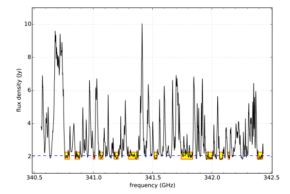
Figure 1.— Spectrum of Orion-KL in spectral window 2 of Band 7, illustrating the difficulty of finding “line free” spectral channels. Shaded boxes indicate the spectral ranges that were included in the continuum map. This spectrum is the scalar average of the interferometric visibility amplitudes obtained on projected baselines shorter than 200 k$\lambda$; it differs from a single dish total power spectrum because it is insensitive to emission that is uniform on spatial scales $>2$ ″.

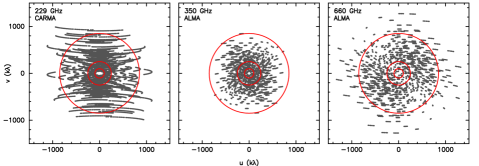
Figure 2.— $(u,v)$ coverage of the data. The 229 GHz data are from the CARMA A and B arrays (Plambeck et al., 2013). Red circles indicate radii of 100, 250, and 850 k$\lambda$.

2.1. Identifying Line-Free Channels

To produce continuum images it is necessary to omit spectral channels that are contaminated by molecular line emission, a challenging task for a chemically rich region such as Orion. We identified such channels by plotting the scalar average of the interferometric visibility data. An example is shown in Figure 1. High amplitudes in this spectrum indicate that the source has brightness variations on scales of 0$\farcs$5–2″ due to the presence of molecular lines. We note that this average does not contain total power data, so it is not the same as the spectrum that one would observe with a single dish; for example, an optically thick line with relatively uniform brightness across the primary beam would not be prominent in the scalar visibility average.

It was more difficult to identify line-contaminated channels in Band 9 using this technique because ozone lines in the earth’s atmosphere increase the system noise temperature, producing broad, cuspy peaks in the spectral noise floor. We note that Band 9 also uses double sideband receivers, so that ozone lines in either sideband generate these noise peaks, although astronomical signals from only one sideband are present.

We adjusted the list of line-contaminated channels after generating a preliminary set of channel images and inspecting the spectrum of SrcI.

2.2. Self-Calibration

After flagging the line-contaminated channels, we averaged the remaining channels in each spectral window into a single channel for continuum imaging. A separate image was generated for each spectral window, omitting visibility data from projected baselines shorter than 250 k$\lambda$ (corresponding to a fringe spacing of 0.82″) in order to filter out extended emission. Data were weighted using Briggs robust=0. The images were dominated by emission from SrcI at the center.

Two iterations of phase-only self-calibration were then applied to the data. The images were deconvolved with the CLEAN algorithm, then self-calibrated using CLEAN components stronger than 3$\sigma$ as a source model. The self-calibration interval was chosen to be 6.05 secs, equal to the integration time. Self-calibration corrects the data for atmospheric phase fluctuations that occur on time scales longer than this. We judged the quality of the self-calibration by comparing, for each 6.05-sec integration, the antenna-based phase corrections derived independently for the 4 spectral windows. The mean phase difference between pairs of bands ranged from 0 to 4°; perfect agreement is not expected since atmospheric delays produce chromatic phase differences. The rms scatter about the mean ranged from 3° to 8°, which indicates that the signal to noise of the calibration procedure is high. Self-calibration increased the flux density of SrcI by approximately 25% at 350 GHz and 50% at 660 GHz. For both Band 7 and Band 9, the flux density in each of the 4 spectral windows was within 3% of the mean, suggesting that no window was seriously contaminated by molecular line emission.

We did not use amplitude self-calibration because for some antennas this yielded unreasonably large (up to 50%) gain drifts on time scales of 20 minutes, probably because of contributions from poorly sampled large scale structures to the visibility amplitudes.

2.3. 229 GHz CARMA Data

To compare continuum flux densities and source sizes over a wide frequency range, we also make use of 229 GHz Orion observations obtained with the Combined Array for Research in Millimeter Astronomy (CARMA) A and B arrays in 2009 and 2011. Maps based on these data were previously published by Plambeck et al. (2013), but here we combine the A and B array data to match the spatial frequency range of the ALMA data as closely as possible. Details of the CARMA calibrations may be found in Plambeck et al. (2013); a 2 minute time interval was used for the final phase-only self-calibration on Orion.

Figure 2 compares the (u,v) coverage (sampling in the spatial frequency domain) for the 3 datasets. The CARMA data are observations over full $(u,v)$ tracks, while the ALMA data are snapshot observations. The 660 GHz data provide the highest angular resolution; 350 GHz, the lowest.

Table 2Gaussian Fits to SrcI

freq	synth beam	$\alpha$(J2000)	$\delta$(J2000)	epoch	integrated flux	deconvolved size	P.A.
(GHz)	(arcsec, P.A.)	(h m s)	(° ′ ″)		(mJy)	(arcsec)	(°)
243	$0.06\times 0.04$, $3\arcdeg$	05 35 14.5141	-05 22 30.575	2009.1	$11\pm 2$	$0.23\pm 0.01\times 0.12\pm 0.01$	$142\pm 2$
229	$0.18\times 0.15$, $72\arcdeg$	05 35 14.5136	-05 22 30.584	2009.1	$330\pm 50$	$0.21\pm 0.02\times 0.07\pm 0.03$	$140\pm 2$
349	$0.25\times 0.18$, $66\arcdeg$	05 35 14.5152	-05 22 30.564	2014.6	$790\pm 80$	$0.24\pm 0.03\times 0.07\pm 0.06$	$140\pm 1$
661	$0.16\times 0.12$, $-50\arcdeg$	05 35 14.5129	-05 22 30.576	2014.5	$3455\pm 520$	$0.25\pm 0.02\times 0.08\pm 0.02$	$142\pm 1$

3. CONTINUUM IMAGES

Figure 3.— Comparison of SrcI continuum images at 229, 349, and 661 GHz. The 229 GHz data are from CARMA. Left-hand panels show images deconvolved with CLEAN; the synthesized beam sizes are given in Table 2. Right-hand panels show images that were deconvolved with a maximum entropy algorithm; these have not been convolved with a restoring beam. The contour levels are ($\pm 2.5$, 5, 10, 20, $\dots$ 90%) of the peak flux densities, which are 0.19, 0.52, 1.68 Jy/beam (at 229, 349, 661 GHz) for the CLEAN images, and 7.8, 12, and 76 mJy/pixel (0$\farcs$25 $\times$ 0$\farcs$25 pixels) for the MAXEN images.

Figure 3 displays continuum images of SrcI centered at frequencies of 229, 349, and 661 GHz that were generated from the self-calibrated data on baselines $>$250 k$\lambda$, using robust=0 weighting. The channel-averaged visibilities for the 4 separate spectral windows were combined using multifrequency synthesis to avoid bandwidth smearing at the edge of the images. Each image covered a field of view greater than the FWHM of the telescope primary beamwidth, but Figure 3 shows only a 1″ box centered on SrcI.

The images on the left were deconvolved with CLEAN, those on the right with a maximum entropy algorithm (Miriad task MAXEN). The MAXEN images are super-resolved in the sense that they have not been convolved with a restoring beam. Since MAXEN attempts to produce the flattest map that is consistent with the data, the results are sensitive to the noise level that is estimated for the data—we used the rms noise measured from the CLEAN residual map. The flux densities were left unconstrained in the MAXEN images.

To measure SrcI’s size and integrated flux density, we fit both Gaussian and disk models to the emission in the central 0$\farcs$8 box of the images using Miriad program imfit. We judged the quality of each fit from the rms noise in this box after subtracting the model image. There was little difference in the residual noise between Gaussian and disk models, so we discuss only the results of the Gaussian fits here. Table 2 summarizes these results. For comparison, the table also includes the 43 GHz source parameters derived by Goddi et al. (2011) from VLA images.

SrcI is considerably narrower than the synthesized beams, so our measurements of the minor axis are particularly uncertain. For all 3 frequencies we found that deconvolved widths fitted to the CLEAN images were smaller than those measured from MAXEN images, or to widths fitted directly to the $>$250 k$\lambda$ visibility data with program uvfit. For example, at 229 GHz the CLEAN, uvfit, and MAXEN minor axis widths were 0$\farcs$047, 0$\farcs$072, and 0$\farcs$105, respectively. Therefore, in Table 2 we give the average of the sizes obtained with these 3 methods; uncertainties are estimated from the scatter in the results.

For the measured source sizes, the integrated flux densities correspond to peak brightness temperatures of approximately 500 K. Uncertainties in the integrated fluxes are dominated by the absolute calibration uncertainties of $\pm~{}10$% for Band7 and $\pm$ 15% for Band 9, as given by the ALMA Cycle 1 Technical Handbook, and of $\pm$ 15% estimated for the 230 GHz CARMA data.

The absolute positions of SrcI at 349 and 661 GHz differ by ($-18,+34$) and ($-52,+22$) milliarcseconds from SrcI’s expected position in 2014 July, $05^{\rm h}35^{\rm m}14\fs 5164$, $-5\arcdeg 22\arcmin 30\farcs 598$, predicted from the 43 GHz position and proper motions given by Goddi et al. (2011). Since the ALMA data are snapshot observations obtained with a single phase calibrator, not optimized for astrometry, we consider this to be reasonable agreement.

The 229 GHz flux density in Table 2, $330\pm 50$ mJy, is larger than the value $310\pm 45$ mJy that we reported previously (Plambeck et al., 2013, Table 1); the new value is derived from combined CARMA A and B array data, whereas the old value was based on A array data alone.

The spectral energy distribution of SrcI from cm to submm wavelengths will be discussed later, in Section 5.1.

Figure 4.— Spectra of SrcI in the four Band 7 spectral windows, generated from channel maps with an 0$\farcs$28$\times$0$\farcs$24 synthesized beam. The spectral window is labeled outside the upper right corner of each panel. The frequency scale is in the frame of the source, at V_LSR=5 $\rm km~{}s^{-1}$. The velocity resolution is 1.65 $\rm km~{}s^{-1}$. Flux densities are integrated over an 0$\farcs$2$\times$0$\farcs$2 box centered on SrcI. Blue horizontal dashed lines indicate the continuum levels. Selected spectral lines are annotated; their frequencies and upper state energy levels E_U are given in Table 3. Each line is shaded over a velocity interval of 36 $\rm km~{}s^{-1}$ centered on the line frequency; yellow shading indicates E${}_{\rm U}>500$ K; green, E${}_{\rm U}<500$ K.

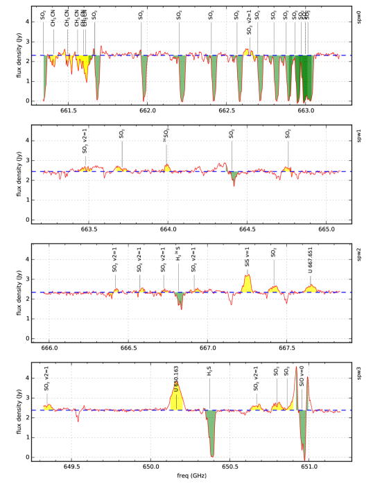
Figure 5.— Same as Figure 4 for the four Band 9 spectral windows. For these maps the synthesized beam was 0$\farcs$18$\times$0$\farcs$14, and the effective velocity resolution plotted here is 1.8 $\rm km~{}s^{-1}$. Frequencies and upper state energies for the annotated spectral lines are given in Table 4.

4. SPECTRAL LINES

Spectral channel images were generated from the self-calibrated visibility data using baselines $>100$ k$\lambda$ and robust=0 weighting. Including data from baselines shorter than 250 k$\lambda$ slightly degrades the angular resolution relative to the continuum images, but improves the signal to noise ratio. Figures 4 and 5 display the spectra integrated over a 0$\farcs$2$\times$0$\farcs$2 box centered on SrcI. These spectra have been Hanning-smoothed to an effective velocity resolution of 1.7 $\rm km~{}s^{-1}$. The frequency axes are computed for a source velocity V_LSR=5 $\rm km~{}s^{-1}$. This is the velocity of SrcI determined from previous observations of SiO masers and H₂O lines (e.g., Wright et al., 1995; Hirota et al., 2016). The blue horizontal dashed line in each panel indicates the continuum flux density obtained from an average of the line-free channels in that spectral window. These flux densities are lower than those listed in Table 2 because the 0$\farcs$2$\times$0$\farcs$2 box does not completely cover the source.

Table 3Band 7 Spectral lines

freq	molecule	EU
(GHz)		(K)
340.6119	29SiO v=1	1832
340.7142	SO	81
340.8387	33SO	87
341.2755	SO2	369
341.3233	SO2	1412
341.4031	SO2	808
341.5594	SO v=1	1686
341.6133	S18O	156
341.6740	SO2	679
342.2089	34SO2	35
342.3320	34SO2	110
342.4359	SO2 v2=1	1041
342.5044	SiO v=2	3595
342.6476	CO v=1	3117
342.7616	SO2	582
342.8829	CS	66
342.9808	29SiO v=0	74
343.1010	SiS v=1	1236
343.4767	SO2	2068
343.8294	SO v=1	1677
343.9237	SO2 v2=1	1058
344.2001	HC15N	41
344.2453	34SO2	89
352.9780	unknown
353.6480	unknown
354.4604	HCN v2=1	1067
354.5055	HCN	43
354.6242	SO2 v2=1	1852
354.6975	HC3N	341
354.8000	SO2 v2=1	928
355.0455	SO2	111
355.1865	SO2	180
355.5711	S18O	93
355.7055	SO2	1143
356.0406	SO2	230
356.2222	34SO2	320
356.2556	HCN v2=1	1067

Table 4Band 9 Spectral Lines

freq	molecule	EU
(GHz)		(K)
649.3467	SO2 v2=1	2037
650.1630	unknown
650.3742	H2S	282
650.6693	SO2 v2=1	1580
650.7967	SO2	1075
650.8620	SO2	1090
650.9561	SiO v=0	250
661.3436	SO2	333
661.4088	CH3CN	702
661.4968	CH3CN	652
661.5597	CH3CN	616
661.5975	CH3CN	595
661.6101	CH3CN	588
661.6683	SO2	313
661.9622	SO2	295
662.2027	SO2	277
662.4043	SO2	261
662.5669	SO2	245
662.6479	SO2 v2=1	1443
662.6976	SO2	230
662.7995	SO2	217
662.8770	SO2	204
662.9336	SO2	192
662.9728	SO2	181
662.9977	SO2	171
663.0144	SO2	146
663.4789	SO2 v2=1	1476
663.7109	SO2	1496
663.9904	34SO2	772
664.4047	SO2	217
664.7604	SO2	921
666.4179	SO2 v2=1	1411
666.5734	SO2 v2=1	1380
666.7238	SO2 v2=1	1284
666.8162	H234S	245
666.9162	SO2 v2=1	1899
667.2525	SiS v=1	1680
667.4198	SO2	1649
667.6510	unknown

A multitude of molecular lines are evident in the spectra. These include many narrow absorption features that originate in relatively cool (T $\lesssim 200$ K) foreground gas that is not in close proximity to SrcI. It is beyond the scope of this paper to identify all of these lines. The velocity of the absorbing gas is uncertain by a few $\rm km~{}s^{-1}$, so often a feature matches 5 or 10 candidate transitions in the Splatalogue spectral line database. Only a global fit to the entire spectrum, to confirm that all expected transitions of a given molecule are present, can winnow out the most likely identifications.

Here we are primarily interested in broad ($\Delta$v $\gtrsim 30$ $\rm km~{}s^{-1}$) spectral features that originate from SrcI or its outflow. Many of these lines are identified in Figures 4 and 5; their rest frequencies and upper state energy levels are given in Tables 3 and 4. Sulfur- and silicon-rich molecules such as SiO, SO, SO₂, SiS, and H₂S are particularly prominent. A few lines do not match any plausible transitions in the Splatalogue database; they are listed in boldface in Tables 3 and 4.

In the figures, transitions with upper state energies E${}_{\rm U}<500$ K are shaded in green; these appear mainly in absorption against the SrcI continuum. Transitions with E${}_{\rm U}>500$ K are shaded in yellow; these appear mainly in emission. The shaded widths are 36 $\rm km~{}s^{-1}$ in all cases, equal to the full width of the SiO or H₂O maser emission from SrcI (e.g., Genzel et al., 1981; Wright et al., 1995).

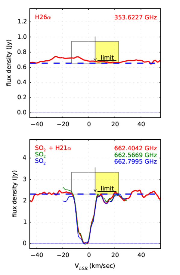
Figure 6.— SrcI spectra centered on the H26$\alpha$ and H21$\alpha$ recombination line frequencies. As in Figures 4 and 5, flux densities are summed over 0$\farcs$2$\times$0$\farcs$2 boxes centered on SrcI. Black arrows indicate the expected line center velocities; gray rectangles, the expected linewidths. In the top panel, an unidentified emission line centered at -18 $\rm km~{}s^{-1}$ intrudes into the H26$\alpha$ rectangle. In the bottom panel, the 17(7,11)-17(6,12) transition of SO₂ coincides exactly with the recombination line frequency, but SO₂ absorption obscures only the blueshifted half of the H21$\alpha$ rectangle; spectra of two neighboring SO₂ lines are overplotted for comparison. Upper limits on the recombination line intensities are based on the redshifted velocity ranges indicated by shading.

4.1. Hydrogen Recombination Lines

A primary goal of the ALMA observations was to search for emission from the H26$\alpha$ and H21$\alpha$ recombination lines, at 353.6228 and 662.4042 GHz respectively. A detection of either transition would confirm the presence of ionized hydrogen in SrcI, strongly bolstering the case that the source is a hypercompact HII region.

Figure 6 displays 100 $\rm km~{}s^{-1}$ wide slices of the SrcI spectrum centered on the recombination line frequencies. We expect that, if present, the recombination lines would be centered at V_LSR $\sim 5$ $\rm km~{}s^{-1}$ with widths $\geq 36$ $\rm km~{}s^{-1}$, similar to the molecular emission lines. This velocity range is indicated by the light gray rectangle in each panel. There are no indications of emission peaks at the expected frequencies, although neither spectrum is perfectly clean—in the upper panel, a weak, unidentified emission line at 353.648 GHz intrudes into the blueshifted portion of the H26$\alpha$ rectangle, while in the lower panel, strong absorption by the 17(7,11)–17(6,12) transition of SO₂ at 662.4043 GHz obscures the blueshifted half of the H21$\alpha$ rectangle.

One might expect that it would be impossible to set an upper limit on the strength of the H21$\alpha$ line, since the interfering SO₂ transition coincides with it almost perfectly in frequency. However, as discussed in Section 4.3 below, SO₂ absorption originates primarily in the outflow from SrcI, so it affects only blueshifted velocities. For V_LSR$>5$ $\rm km~{}s^{-1}$ the outflowing gas lies primarily behind SrcI, so it should not attenuate recombination line emission from the source. The 17(7,11)-17(6,12) transition is one of a series of SO₂ lines near 662 GHz with similar line strengths and upper state energy levels. The spectra of two neighboring lines, the 16(7,9)-16(6,10) and 14(7,7)-14(6,8) transitions, are overlaid in Figure 6 to demonstrate the similarity of the three SO₂ line profiles. There is no excess emission in the redshifted wing of the 17(7,11)-17(6,12) line that that could be attributed to H21$\alpha$.

We use the redshifted velocity range $5<$ V_LSR$~{}<23$ $\rm km~{}s^{-1}$ (shaded in Figure 6) to establish upper limits on the intensities of the recombination lines. As shown by the horizontal black lines in each spectrum, all channels within this velocity range have line + continuum flux densities that are $<~{}1.05~{}\times$ the mean continuum level. This limit on the line-to-continuum ratio will be used in Section 5.2 to argue that free-free emission is not a viable explanation for SrcI’s continuum.

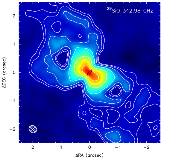
Figure 7.— Map of the v=0, J=8-7 line of ²⁹SiO over the velocity range $0<$V_LSR$<10$ $\rm km~{}s^{-1}$, showing the bipolar outflow from SrcI. The synthesized beam, shown in the lower left corner, is 0$\farcs$29$\times$0$\farcs$25 at PA 58°. The contours are 0.05, 0.1, 0.2, 0.4, 0.8, 1.6 Jy/beam (7.3 to 230 K). The black, 0$\farcs$23 $\times$ 0$\farcs$07 ellipse at the center shows the size and location of the model continuum disk.

4.2. Bipolar Outflow

Previous observations (e.g., Plambeck et al., 2009; Niederhofer et al., 2012; Greenhill et al., 2013) have established that the bipolar outflow from SrcI is most clearly visible in images of SiO lines in the v=0 vibrational state. Our data include two such transitions, the J=8-7 ²⁹SiO line at 342.981 GHz and the J=15-14 SiO line at 650.956 GHz. The lower frequency, J=8-7, data contain more short antenna spacings (see Figure 2), so do a better job of sampling the large scale structure of the outflow. An image of this transition integrated over the velocity range $0<$V_LSR$<10$ $\rm km~{}s^{-1}$ is shown in Figure 7. All the visibility data, down to the shortest, 35 k$\lambda$ baselines, were used to make this image. No other lines in our data show this extended bipolar pattern.

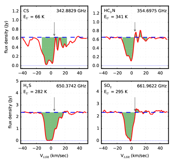
Figure 8.— Examples of molecular lines exhibiting blueshifted absorption by the SrcI outflow. Line frequencies and upper energy levels are given. As in Figures 4 and 5, flux densities are summed over 0$\farcs$2$\times$0$\farcs$2 boxes centered on SrcI, and the dashed blue lines indicate the continuum levels. Arrows indicate the LSR velocity of SrcI, 5 $\rm km~{}s^{-1}$; 36 $\rm km~{}s^{-1}$ wide ranges centered on this velocity are shaded.

4.3. Absorption Lines

Almost all of the lines with upper state energies E${}_{\rm U}<500$ K appear in absorption against the SrcI continuum. The absorption is highly asymmetric. It is limited primarily to blueshifted ($-13<$ V_LSR$<5$ $\rm km~{}s^{-1}$) velocities; i.e., it originates in gas that is moving toward us from SrcI. Figure 8 shows several examples. Since the velocity width of the absorption is comparable with the halfwidth of the SiO v=0 emission, we associate it with material within the SrcI outflow, rather than from unrelated foreground gas along the line of sight.

Although absorption is apparent in lines of many abundant molecules like HCN, HC¹⁵N, and HC₃N, it is especially prominent in transitions of sulfur-bearing species such as SO, SO₂, H₂S, and their isotopologues.

In 1$\farcs$5 resolution ALMA Band 6 science verification data, Wu et al. (2014) found evidence for redshifted CH₃OH absorption toward SrcI, indicative of infall. Presumably this infall occurs in the outer layers of the Kleinmann-Low Nebula, on angular scales $\gtrsim\,$3″ that are poorly sampled by our observations.

4.4. Emission Lines

Lines with upper state energy levels E${}_{\rm U}>500$ K, shaded in yellow in Figures 4 and 5, almost always are seen in emission. Generally these lines are symmetric about V_LSR=5 $\rm km~{}s^{-1}$, with full widths of 30-40 $\rm km~{}s^{-1}$. Most of them can be identified with transitions of the molecules SO, SO₂, SiS, and SiO, often in excited vibrational states. We believe that the line identifications are correct because essentially all of the stronger transitions of these molecules that are listed in the Splatalogue database correspond to emission features in the spectra. For example, within the frequency ranges covered by our observations, the Splatalogue lists 10 SO₂ transitions in the ground vibrational state with intensities $>10^{-5}$ (at 300 K) and upper state energies between 500 and 2500 K. Of these, 8 are detected. The undetected transitions are at 650.862 GHz, buried under the wing of the bright SiO v=0 line, and at 661.511 GHz, amidst a jumble of CH₃CN absorption features. Similarly, we detect 12 out of 16 strong SO₂ transitions in the v2=1 vibrational level.

Of the $>30$ identified emission lines, all but two have upper state energy levels between 500 and 2100 K. The two exceptions are the v=1, J=3-2 CO line at 342.648 GHz (E_U = 3117 K) and the v=2, J=8-7 SiO line at 342.504 GHz (E_U = 3595 K). These upper state energies are comparable to those of the vibrationally excited H₂O lines at 232.687 GHz (E_U = 3462 K) and 336.228 GHz (E_U = 2955 K) previously identified by Hirota et al. (2012, 2014) in SrcI.

Four of the emission lines are unidentified. The strongest of these is a broad (fullwidth 50 $\rm km~{}s^{-1}$), centrally peaked feature at 650.163 GHz. As shown in Figure 9, the position-velocity diagram of this line is similar to those of the SiO v=1 and v=2 lines, hinting that it may originate from a vibrationally excited transition with $E_{\rm U}>2500$ K.

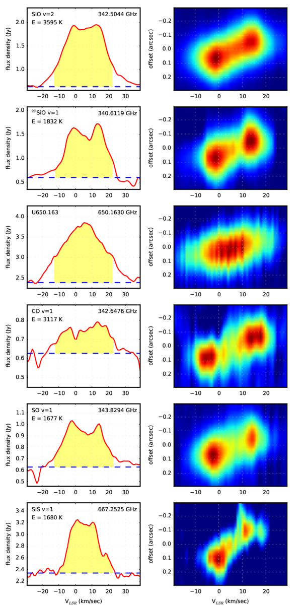
Figure 9.— Spectra and position-velocity plots for selected emission lines. As in previous figures, spectra are integrated over an 0$\farcs$2 box centered on SrcI, and are shaded over a 36 $\rm km~{}s^{-1}$ range centered at V_LSR=5 $\rm km~{}s^{-1}$. Position-velocity diagrams are measured along the major axis of the SrcI disk, at PA 142°; negative offsets are to the NW, positive offsets to the SE. The continuum was subtracted from the spectral line channel images before generating the position-velocity plots.

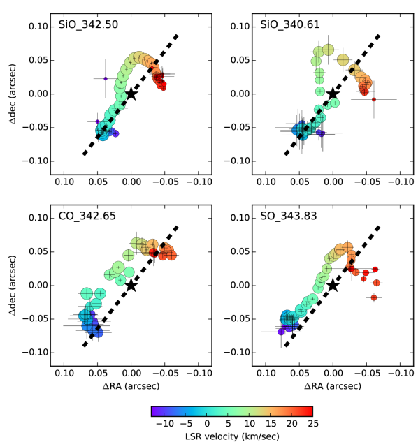
Figure 10.— Velocity centroid maps for selected spectral lines. The area of each circle is proportional to the flux in that channel; colors indicate the radial velocity. The 0$\farcs$23 long dotted line in each panel represents the midplane of the continuum disk.

4.5. Central Mass Estimate

Figure 9 presents spectra of 6 of the brightest emission lines, and the corresponding position-velocity diagrams measured along the major axis of the continuum disk, at PA 142°. All the lines show a velocity gradient along the disk. Except for U650.163, the spectra are double-peaked, and the brightest emission is offset by 0.05-0.10″ from the origin. The double-peaked line profiles and the absence of high velocity gas toward the central position suggest that molecular line emission originates from a torus or ring, rather than a filled disk.

Figure 10 plots the position centroids of individual 1 $\rm km~{}s^{-1}$ wide spectral channels for 4 selected molecular lines. The offsets were derived from 2-dimensional Gaussian fits to 0$\farcs$26 resolution images. Centroids are plotted only for channels where the fits have formal uncertainties smaller than 0$\farcs$03. The 0$\farcs$23-long dotted line at PA 142° in each panel represents the midplane of the continuum disk. These plots resemble the centroid map of the 336 GHz transition of vibrationally excited H₂O (Hirota et al., 2014), and are consistent with the much higher resolution SiO maser spot maps (Kim et al., 2008; Matthews et al., 2010). The highest velocity gas tends to be localized along the edges of the bipolar outflow.

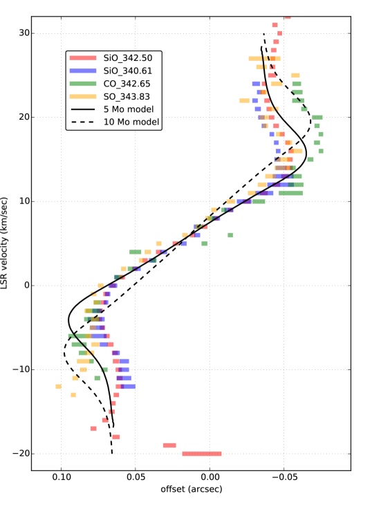
Figure 11.— Position-velocity diagrams along the disk midplane for the spectral lines shown in Figure 10. Horizontal bars indicate the $\pm 1\sigma$ formal errors in the position offsets. Model rotation curves for 5 $\hbox{M}_{\odot}$ and 10 $\hbox{M}_{\odot}$ central objects are shown by solid and dashed lines. The model assumes optically thin emission from gas in a rotating, edge-on ring with 20 AU inner radius, 50 AU outer radius, and 4 $\rm km~{}s^{-1}$ turbulent linewidth.

Figure 12.— Comparison of spectral line (halftone images, thin black contours) and 661 GHz continuum emission (thick red contours) toward SrcI. Top panels show the SiS transition at 667.252 GHz (contour levels 0.04, 0.08, $\ldots$, 0.28 Jy/beam); bottom panels show the unidentified spectral line at 650.163 GHz (contour intervals 0.05, 0.1, 0.2, $\ldots$, 0.8 Jy/beam). Each channel map covers a 12 $\rm km~{}s^{-1}$ wide interval centered at the LSR velocity indicated in the upper left corner. The continuum contours are 0.5, 1.0, 1.5 Jy/beam. The continuum has been subtracted from each spectral channel. The FWHM of the synthesized beam, 0$\farcs$16$\times$0$\farcs$12, is shown by the hatched blue ellipse in the lefthand panels. Spectral line emission extends above and below the continuum disk.

We projected the channel centroids in Figure 10 onto the disk midplane in order to generate the rotation curves shown in Figure 11. To estimate the mass of the central object, we simulated these rotation curves using a model similar to the one used by Hirota et al. (2014). The model assumes optically thin emission from gas in Keplerian rotation around a central point mass. The gas has uniform temperature and density, and is confined to a ring that is viewed exactly edge-on. We fixed the outer radius of the ring to 50 AU to match the radius of the continuum disk, but experimented with different inner radii. A turbulent linewidth of 4 $\rm km~{}s^{-1}$ was assumed. For each velocity we numerically integrated the emission from all cells in the ring in order to compute the offset of the emission centroid from the origin.

Note that, although the spectral line profiles are symmetric around V_LSR$\sim$5 $\rm km~{}s^{-1}$, the blueshifted channel centroids typically lie farther from the origin than the redshifted centroids, so that the dynamical center of rotation used by the model is 0$\farcs$015 (6 AU) from the center of the continuum source. Higher angular resolution is required to see if this offset is real.

We modeled the rotation curves for a range of central masses and inner radii. Central masses of 5-7 $\hbox{M}_{\odot}$ matched the data best, particularly for offsets $<$0$\farcs$05 where the rotation curves of all 4 spectral lines are consistent. Figure 11 shows the model results for 5 $\hbox{M}_{\odot}$ and 10 $\hbox{M}_{\odot}$ central objects and an inner ring radius of 20 AU. The 10 $\hbox{M}_{\odot}$ simulation (dashed) is steeper than the observed rotation curve at small radii. This is similar to the result obtained by Hirota et al. (2014) for the 336 GHz H₂O line in SrcI.

Of course the model is highly idealized, particularly since it utilizes centroids to represent emission regions that are unresolved by the synthesized beam. However, an estimated central mass of 5-7 $\hbox{M}_{\odot}$ is consistent with that derived by Matthews et al. (2010) from high resolution SiO maser maps. The central mass could be larger if the plane of the disk is inclined with respect to the line of sight, but the observed axial ratio of the continuum source, 0$\farcs$23 : 0$\farcs$07, implies that the disk is tilted by no more than about 20°, which changes the central mass by less than 10 percent.

4.6. Outflow or Disk Midplane Emission?

Hirota et al. (2014) inferred that the 336 GHz H₂O line was emitted from hot gas in the midplane of the SrcI disk because the velocity channel centroids for this line were tightly clustered along the major axis of the continuum disk. Their observations were made with an 0$\farcs$4 beam, however. In contrast, VLBI observations with 0.5 millarcsecond resolution show that 43 GHz SiO masers avoid a 0.05″ wide band along the disk midplane (Kim et al., 2008; Matthews et al., 2010).

Although our images have inadequate resolution to say whether line emission avoids the disk midplane, they do clearly show that line emission is spatially extended relative to the continuum. This is evident in Figure 12, which overlays Band 9 line channel maps and continuum contours. These images were generated from visibilities measured on baselines longer than 300 k$\lambda$ in order to obtain 0$\farcs$13 resolution along the minor axis of the disk. The continuum has been subtracted from each line channel. The velocity gradient along the major axis of the disk is clearly apparent. Because line emission extends outward from the top and bottom surfaces of the disk, we associate it with the base of the bipolar outflow, or with the atmosphere of the disk.

In Sections 5.4 and 5.5 we argue that the continuum radiation from the disk is mostly thermal emission from warm dust, and hypothesize that SiO masers originate on the surface of the disk where dust grains are destroyed. Thus, it’s possible that emission from silicon- and sulfur-rich molecules like SiS, SO, and SO₂ is limited primarily to the disk surface, while the H₂O line mapped by Hirota et al. (2014) originates mostly from the disk interior.

Table 5SO₂ Integrated Intensities

EU	frequency	S${}_{\rm ij}\mu^{2}$	$\int T_{R}dv$
(K)	(GHz)	(D2)	(K-km/sec)
v = 0 vibrational level
582	342.762	50.74	221 (6)
679	341.674	68.31	366 (6)
808	341.403	71.97	178 (6)
921	664.760	31.35	107 (20)
1075	650.797	47.15	148 (20)
1143	355.705	14.61	71 (6)
1649	667.420	89.22	30 (20)
2068	343.477	21.36	83 (6)
v2 = 1 vibrational level
928	354.800	23.77	261 0(6)
1041	342.436	29.58	79 0(6)
1058	343.924	19.56	49 0(6)
1443	662.648	52.58	52 (20)
1476	663.479	54.57	91 (20)
1580	650.669	60.99	87 (20)
1852	354.624	102.36	93 0(6)
2037	649.347	85.49	61 (16)

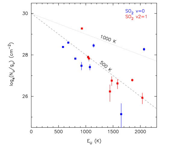
Figure 13.— Rotational energy diagram for SO₂ emission lines in an 0$\farcs$2 box centered on SrcI. Spectral line parameters are given in Table 5; note that integrated intensities were computed using only the redshifted velocity range 5-20 $\rm km~{}s^{-1}$. The slope of the dashed line corresponds to an excitation temperature of 500 K; the dotted line, 1000 K.

4.7. Excitation Temperature Analysis

The detection of CO, SiO, and H₂O lines from vibrationally excited energy levels indicates that some 3000 K gas exists in SrcI. However, a rotational diagram analysis of the SO₂ emission lines suggests that the mean excitation temperature is considerably lower. Our spectra contain 16 SO₂ lines with E${}_{\rm U}>600$ K that appear not to be seriously corrupted by foreground absorption. Eight of these are in the ground vibrational state, and eight are in the v2=1 bending mode vibrational level. A rotational diagram analysis (e.g. Blake et al., 1987) assumes that the lines are optically thin, that they originate in the same column of gas, and that the rotational energy ladders are in local thermodynamic equilibrium. The SO₂ v2=1 level lies only 745 K above the ground state (Müller & Brünken, 2005), so we will assume that the v=0 and v2=1 rotational ladders are thermalized at the same temperature.

Table 5 lists the upper energy level E_U, frequency, line strength $\mu^{2}S$, and integrated intensity in K-$\rm km~{}s^{-1}$ for each of the SO₂ lines. The integrated intensity $W=\int T_{R}(v)dv$ is computed from the (continuum-subtracted) radiation temperatures averaged over the velocity range 5$\,\leq\,$V_LSR$\,\leq\,$20 $\rm km~{}s^{-1}$, in a 0$\farcs$2$\times$0$\farcs$2 box centered on SrcI; uncertainties are estimated from line-free channels. We restrict the analysis to redshifted velocities because we expect that this emission originates primarily from the outflow on the far side of SrcI (see discussion in Section 4.3), so we do not have to take into account molecular absorption of continuum photons from SrcI.

For each line we calculate the quantity $3kW/(8\pi^{3}\nu S\mu^{2})=N_{u}/g_{u}$, the column density per molecular sublevel, where $k$ is Boltzman’s constant and $g_{u}$ is the degeneracy of the upper energy level. A plot of natural log of $N_{u}/g_{u}$ against $E_{u}$ should produce a straight line with slope $1/T_{\rm ex}$ and intercept $N(SO_{2})/Q(T_{ex})$, where $Q(T_{ex})$ is the rotational partition function at excitation temperature $T_{ex}$. This plot is shown in Figure 13. The slope of the dashed line corresponds to an excitation temperature of 500 K, and the intercept corresponds to an SO₂ column density N(SO₂) = $2\times 10^{17}$ cm^-2, where we have taken $Q(500~{}K)=15611$, the combined partition function for the v=0 and v2=1 vibrational states, from the Cologne Spectral Line Database. Although there is a great deal of scatter in the plot, it appears that little of the gas is at temperatures greater than about 1000 K (dotted line in Figure 13).

5. DISCUSSION

The observations described above provide important clues to the nature of SrcI. We first consider the origin of the radio continuum, concluding that it is primarily thermal dust emission from a disk or torus, optically thick even at frequencies as low as 43 GHz. We then compare the measured properties of SrcI with the predictions of the dynamical decay model.

5.1. Continuum Spectral Energy Distribution

Figure 14 plots the continuum flux densities measured for SrcI from 4 to 690 GHz. The results from this paper are shown as red squares. The remaining data are from the compilation in Table 2 in Plambeck et al. (2013), supplemented by recent VLA (Rivilla et al., 2015; Forbrich et al., 2016) and ALMA (Hirota et al., 2015, 2016) results. Error bars are shown for all the points, but often are smaller than the size of the plot symbols.

The scatter in the flux densities at mm and submm wavelengths ($\nu\gtrsim 100$ GHz) is indicative of the difficulty in making these measurements. SrcI is an extended object, not a true point source, and it is embedded in a clumpy ridge of dust emission. When observed with a $>1$″ FWHM synthesized beam it appears merely as a protrusion on the Hot Core dust ridge—see, e.g., Tang et al. (2010), Figure 1, or Plambeck et al. (2013), Figure 1. Even with subarcsecond angular resolution, the images can be corrupted by negative sidelobes from extended structures that are not fully sampled by the aperture synthesis observations. The well-sampled, 0$\farcs$2 resolution, ALMA and CARMA data described in this paper provide the most reliable measurements to date at these wavelengths.

Source variability may also be responsible for some of the scatter in Figure 14. Plambeck et al. (2013) presented tentative evidence that SrcI has brightened relative to BN at 43 and 86 GHz since 1995, and Rivilla et al. (2015) found indications of variability on time scales of just a few hours at 34 GHz.

As shown by the solid line in Figure 14, SrcI’s flux density scales approximately as $\nu^{2}$ from 43 GHz to $>$350 GHz, consistent with emission from a blackbody that subtends the same solid angle at all frequencies. The line shows the flux density that one would receive from a 0$\farcs$23 $\times$ 0$\farcs$07 FWHM Gaussian source with a peak brightness temperature of 480 K. Below 43 GHz and above 350 GHz most of the measured flux densities lie above the $\nu^{2}$ curve.

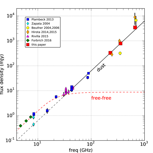
Figure 14.— Spectral energy distribution of SrcI from cm to submm wavelengths. References are given in the legend; red squares indicate the fluxes from this paper. From 43 to $>350$ GHz the data follow a $\nu^{2}$ curve (black line) that is fit to a flux density of 330 mJy at 229 GHz. In Section 5.4 we argue that this emission originates from optically thick dust. At lower frequencies free-free emission (red dashed curve) probably becomes important.

5.2. An Optically Thick Hypercompact HII Region?

Our data convincingly rule out the possiblity that SrcI is a hypercompact HII region. Such an HII region would need to be optically thick even at 660 GHz in order to explain the observed spectral energy distribution and the absence of a detectable H21$\alpha$ recombination line. We find, however, that the Lyman continuum flux required to maintain the ionization of such an HII region could only be generated by a central star with a luminosity that exceeds that of the entire Kleinmann-Low Nebula.

To begin, we estimate the minimum free-free optical depth that would be consistent with the observations. The recombination line and continuum opacities are approximated by (Rohlfs & Wilson, 2000)

$$\tau_{\rm L} \,=\, 1.92\times 10^{3}\,{T_{e}}^{-2.5}\,EM\,/\Delta\nu_{\rm kHz}$$ (1)

$$\tau_{\rm ff} \,=\, 8.24\times 10^{-2}\,T_{e}^{-1.35}\,\nu^{-2.1}\,EM\,a(\nu,T)$$ (2)

where $T_{e}$ is the electron temperature in K, $\nu$ is the frequency in GHz, $EM=\int\!n_{e}^{2}\,dz$ is the emission measure in pc cm^-6, $\Delta\nu_{\rm kHz}$ is the recombination linewidth in kHz, and $a(\nu,T)$ is a correction factor close to unity. For $\nu=662.4$ GHz, $T_{e}=8000$ K, and $\Delta\nu_{\rm kHz}=1.1\times 10^{5}$ ($\Delta v=50$ $\rm km~{}s^{-1}$), these expressions predict $\tau_{\rm L}\sim 5.7\,\tau_{\rm ff}$. Thus, in the optically thin limit the H21$\alpha$ recombination line would be 5.7 times brighter than the free-free continuum. In Section 4.1, however, we set an upper limit on the H21$\alpha$ intensity of 5% of the continuum level, so

$$1-e^{-(\tau_{\rm L}+\tau_{\rm ff})}<1.05\,(1-e^{-\tau_{\rm ff}}).$$ (3)

For $\tau_{\rm L}/\tau_{\rm ff}=5.7$, Equation 3 implies a free-free continuum opacity $\tau_{\rm ff}>3$.

If the path length through SrcI is 100 AU, comparable to its major diameter, and if $\tau_{\rm ff}>3$ and $T_{e}=8000$ K, then equation (2) implies that the electron density $n_{e}>10^{8}$ cm^-3. These numbers yield an excitation parameter $U=r(n_{e}n_{H})^{1/3}>50$ pc cm^-2, which serves as a measure of the flux of ionizing photons from the central star. This corresponds to the excitation parameter expected for a zero age main sequence O7 star with Lyman continuum flux $5\times 10^{48}$ photons s^-1 and total luminosity $>10^{5}$ $\hbox{L}_{\odot}$ (Panagia, 1973). Since this is greater than the luminosity of the entire Kleinmann-Low Nebula, we conclude that SrcI cannot be an HII region.

Note that our analysis does not rule out some small contribution to the continuum from free-free emission, as long as the recombination line intensities are $<\,$5% of the total continuum flux.

5.3. Electron-Neutral Free-Free Emission?

Reid et al. (2007) considered the possibility that SrcI’s continuum might originate from electrons that are scattered by neutral hydrogen atoms or molecules (the so-called H^- and H${}_{2}^{-}$ opacities). This mechanism is important for gas at temperatures between 1000 and 4500 K, in which Na, K, and other metals are collisionally ionized but H and H₂ are mostly neutral. It is thought to explain the radio photospheres of Mira variables (Reid & Menten, 1997). Expressions for the H^- and H${}_{2}^{-}$ absorption coefficients are given by Dalgarno & Lane (1966); Reid & Menten (1997) provide convenient analytical approximations to these expressions. The electron-neutral opacity is roughly 1000 times smaller than the electron-ion opacity, so gas densities $>10^{11}$ cm^-3 typically are required to obtain optically thick emission at mm wavelengths.

As for regular p⁺e^- free-free emission, the H^- and H${}_{2}^{-}$ absorption coefficients are proportional to $\nu^{-2}$, so at sufficiently high frequencies the emission must become optically thin. The spectral energy distribution in Figure 14 shows no sign of flattening at higher frequency, however. Is it possible that in SrcI the electron-neutral emission could be optically thick at frequencies as high as 660 GHz?

Hirota et al. (2015) used the Reid & Menten (1997) approximations to compute the turnover frequency $\nu_{\rm to}$ where the (H${}^{-}+$H${}_{2}^{-}$) optical depth becomes unity, for an 84 AU long path length comparable to the path length through SrcI. To obtain a turnover frequency above 600 GHz for gas at 1000 K requires hydrogen density $n_{\rm H}=n($H + 2H${}_{2})>3\times 10^{15}$ cm^-3. For a 20 AU thick $\times$ 84 AU diameter disk, this corresponds to an absurdly high mass of $>$1000 $\hbox{M}_{\odot}$. The disk mass can be much smaller if the gas is hotter, because the fractional ionization increases steeply as the temperature rises. For gas at 3000 K, the density is $9\times 10^{10}$ cm^-3 and the disk mass is only 0.035 $\hbox{M}_{\odot}$. Such a high temperature is inconsistent, however, with both the continuum brightness temperature and the SO₂ excitation temperature (Section 4.7), both of which are $\lesssim 1000$ K. For a disk with temperature below 1200 K and a mass less than a few $\hbox{M}_{\odot}$, Figure A3 in Hirota et al. (2015) implies that electron-neutral free-free emission cannot be a significant source of opacity at frequencies higher than $\sim$200 GHz.

5.4. Dust?

Thermal radiation from dust is the usual emission mechanism for circumstellar disks at mm and submm wavelengths. Generally the dust emission is assumed to be optically thin, with a flux density that scales as

$$S_{dust}(\nu)\propto\kappa_{\nu}\,N\,B_{\nu},$$ (4)

where $\kappa_{\nu}\propto\nu^{\beta}$ is the absorption coefficient per unit (gas+dust) mass, $N$ is the column density, and $B_{\nu}\propto\nu^{2}$ is the Planck function. Typically $\beta\sim 1$, so one expects the spectral energy distribution to be steeper than $\nu^{2}$ at frequencies where dust emission is dominant.

Earlier measurements suggested that SrcI’s spectral index did steepen at about 230 GHz, which led Beuther et al. (2006) and Hirota et al. (2015) to fit the SED with a mixture of free-free emission, dominant below 230 GHz, and dust emission, dominant above. Our flux density measurements suggest that the spectral index begins to steepen only above 350 GHz, however, and in the sections above we argued that neither p⁺e^- nor electron-neutral free-free emission could contribute significantly to the flux densities at frequencies as high as 230 GHz.

Here we consider an alternative possibility, that SrcI’s continuum emission at mm and submm wavelengths originates from optically thick dust, consistent with the observed $\nu^{2}$ spectrum. We attribute the spectral steepening above 350 GHz to a thin, hot “atmosphere” on the outside of the disk that slightly increases the source size or effective temperature at 660 GHz. Some contribution from H^- or p⁺e^- free-free emission is required to explain the continuum at low frequencies, where the dust emission must ultimately become optically thin. Free-free emission may also account for the central point source that seems to be present in high resolution 43 GHz VLA maps of SrcI (Reid et al., 2007; Goddi et al., 2011). We will assume, however, that most of the 43 GHz continuum is attributable to dust. Reid et al. (2007) argued that this was unlikely on the grounds that molecular lines had not been detected toward the disk, but ALMA data now show that lines are abundant at higher frequencies.

Assuming that the dust emission is optically thick at 43 GHz provides a lower limit to the column density through the disk, and hence the disk mass. We follow the procedure used by Chandler et al. (2005) to estimate the mass opacity of dust $\kappa_{\rm 43\,GHz}$ (cross section per gram of gas plus dust) at 43 GHz. They begin with the opacities $\kappa_{\rm ref}$ (cross section per gram of refractory material) calculated by Ossenkopf & Henning (1994) for the case of coagulated grains with no ice mantles and a gas density $n_{\rm H}$ = 10⁸ cm^-3. At 230 GHz, the lowest frequency tabulated, $\kappa_{\rm ref}=5.86$ cm² g^-1. Extrapolating to 43 GHz assuming $\beta$ = 1.1, and using a gas-to-dust mass ratio of 100, Chandler et al. (2005) estimate $\kappa_{\rm 43\,GHz}=9.3\times 10^{-3}$ cm² g^-1. To obtain optically thick emission through the SrcI disk, we require that

$$\tau_{\rm 43\,GHz}=\kappa_{\rm 43\,GHz}\,n_{\rm H}\,m_{\rm H}\,\mu\,D\gtrsim 1,$$ (5)

where $D\sim 100$ AU is the path length through the disk, $n_{\rm H}=n($H + 2H${}_{2})$ is the hydrogen density, $m_{\rm H}$ is the mass of a hydrogen atom, and $\mu=1.36$ is the ratio of the total gas mass to hydrogen mass. Then we find n${}_{\rm H}\gtrsim 3.2\times 10^{10}$ cm^-3, and a disk mass $\gtrsim$0.02 $\hbox{M}_{\odot}$.

The disk mass could be significantly larger if the dust grains in SrcI are very small, or if they have grown to pebble-size. For grains characteristic of the diffuse interstellar medium, Ossenkopf & Henning (1994) find $\kappa_{\rm ref}=0.31$ cm² g^-1 at 230 GHz. Extrapolating to 43 GHz using $\beta=2$, appropriate for very small grains, and again assuming a gas to dust mass ratio of 100, one finds $\kappa_{\rm 43\,GHz}=1.1\times 10^{-4}$ cm². Equation 5 then implies a hydrogen density n${}_{\rm H}=2.7\times 10^{12}$ cm^-3 and a disk mass of 1.7 $\hbox{M}_{\odot}$. A similar hydrogen density and disk mass are obtained for pebble-sized (10 cm) grains, for which $\kappa_{\nu}\sim 2\times 10^{-4}$ cm² g^-1 for $\nu\gtrsim 43$ GHz (Testi et al., 2001). These mass estimates should be considered upper limits, since they are based on unrealistically small grain opacities. It’s also unlikely that gas densities exceed 10¹¹ cm^-3 on the disk surface, as this would collisionally quench the SiO masers (Lockett & Elitzur, 1992; Goddi et al., 2009). We conclude that the disk mass probably is in the range 0.02-0.2 $\hbox{M}_{\odot}$, but could be as large as 2 $\hbox{M}_{\odot}$ for more extreme dust properties.

As noted above, thermal emission from dust cannot explain the flux densities measured below 43 GHz, many of which exceed the $\nu^{2}$ extrapolation from mm wavelengths. For example, the flux density of SrcI at 33.6 GHz is $\sim$10 mJy (Rivilla et al., 2015), whereas optically thick dust would contribute only 7 mJy at this frequency. H^- free-free emission is likely to be responsible for the excess. The dotted red curve in Figure 14 shows a free-free spectrum with a turnover frequency of 30 GHz that is compatible with the low frequency data.

The infrared spectrum of SrcI, glimpsed in light scattered off nearby reflection nebulosities, indicates that the central object has a 3500-4500 K photosphere (Testi et al., 2010). Although H^- free-free emission from this photosphere must contribute to the continuum, it cannot fully explain the low-frequency excess—even a 4000 K, 8 AU diameter source would contribute less than 1 mJy to the 33.6 GHz flux density. Free-free emission must originate from a larger region, perhaps from the SiO maser zone along the disk surface. Our upper limit on the recombination line intensities also does not rule out a small contribution from regular p⁺e^- free-free emission, perhaps from shock-excited gas in the outflow.

5.5. Source Model

The picture of SrcI that emerges is of a dusty disk or torus with a temperature of $\sim$500 K and a mass of $0.02-0.2$ $\hbox{M}_{\odot}$ that orbits a 5-7 $\hbox{M}_{\odot}$ central star (or binary). A bipolar outflow is launched from the surfaces of the disk. These surfaces must be hotter (1200-1500 K) than the interior of the disk in order to account for the SiO masers and other high excitation lines that occur at the base of the outflow. The high abundance of silicon- and sulfur-bearing molecules in the atmosphere of the disk suggests that dust grains are being destroyed in this layer. In essence, SrcI is an inside-out Mira variable: in a Mira, SiO masers occur just inside the radius where dust condenses, whereas in SrcI the masers occur just outside the radius where dust grains are destroyed.

5.6. Rethinking the Paradigm

We now consider the implications of our data for models of star formation in Orion. Our results are not easily explained by scenarios in which SrcI and BN were ejected by the dynamical decay of a multiple system 500 years ago.

Any model of the Orion-KL region must account for the fact that the Becklin-Neugebauer Object, located just 10″ NW of SrcI, is a runaway B star (Plambeck et al., 1995; Tan, 2004). VLA proper motion measurements (Goddi et al., 2011) show that it is moving to the NW at $26.4\pm 2.1$ $\rm km~{}s^{-1}$ in the frame of the Orion Nebula Cluster. BN’s past trajectory passes close to both SrcI and the Orion Trapezium.

Tan (2004) argued that BN was ejected from the Trapezium roughly 4000 years ago as a result of an interaction with $\theta^{1}$Ori C, a compact binary with a total mass of 45 $\hbox{M}_{\odot}$. Chatterjee & Tan (2012) show that the observed orbital parameters of $\theta^{1}$C closely match the values required to eject BN, and argue that the likelihood that $\theta^{1}$C has these properties purely by chance is $\sim 10^{-5}$.

Surprisingly, however, proper motion measurements indicate that SrcI is moving to the SE at $11.5\pm 2.1$ $\rm km~{}s^{-1}$ (Goddi et al., 2011), almost directly away from BN. Tracing the BN and SrcI proper motion vectors backward, Goddi et al. (2011) find that the projected separation of the 2 stars in the plane of the sky was 50 $\pm 100$ AU just 560 years ago. This discovery led to the alternative model in which SrcI and BN were ejected by the dynamical decay of a multiple system (Rodríguez et al., 2005; Gómez et al., 2008; Goddi et al., 2011).

The dynamical decay model also provides an explanation for the system of high velocity (up to 300 $\rm km~{}s^{-1}$) “bullets,” bow shocks and “fingers” that are visible in lines of H₂, Fe II, and CO, and that appear to emerge from a common center a few arcseconds NW of SrcI (Allen & Burton, 1993; Zapata et al., 2009; Bally et al., 2011, 2015). At one time the finger system was assumed to be a high velocity outflow from SrcI, but now it is recognized as the signpost of an explosive event 500-1000 years ago (Doi et al., 2002; Bally et al., 2011). The bullets are interpreted as dense fragments of circumstellar disks that were torn apart in a stellar encounter and launched into the surrounding cloud (Bally et al., 2015).

Although the dynamical decay model has many attractive features, two observational results are difficult to understand:

1. The mass of SrcI inferred from molecular line rotation curves is only 5-7 $\hbox{M}_{\odot}$, too small to have ejected BN with a speed of 25 $\rm km~{}s^{-1}$.

2. SrcI’s 100 AU diameter, 0.1 $\hbox{M}_{\odot}$ disk is unlikely to have survived the final stellar encounter, and it is too large and too massive to have accreted in the 500 years since SrcI was ejected.

Let us consider these points more carefully. First, is SrcI massive enough to have ejected BN? Goddi et al. (2011) did an extensive series of simulations to test under what circumstances a 10 $\hbox{M}_{\odot}$ star can be ejected with speed $\geq 25$ $\rm km~{}s^{-1}$ from a multiple system similar to the hypothesized BN-SrcI system. The most favorable results were obtained if the initial system contained a single 10 $\hbox{M}_{\odot}$ star and a preexisting (primordial) 20 $\hbox{M}_{\odot}$ binary. In about 40% of these trials, dynamical interactions led to the ejection of both objects, and a hardening of the binary orbit. Sometimes the original binary survived, and sometimes there was an exchange of stars. The increase in binding energy of the binary compensates for the kinetic energy of the runaway stars. Ejections were rare, however, if the initial system did not contain a massive binary. For example, only 1 of 1000 simulations that began with three single 10 $\hbox{M}_{\odot}$ stars resulted in the ejection of a star with speed greater than 25 $\rm km~{}s^{-1}$. And, in simulations that began with an 10 $\hbox{M}_{\odot}$ star and an 11 $\hbox{M}_{\odot}$ binary (10+1 or 8+3 $\hbox{M}_{\odot}$), only 1% of the trials led to an ejection, always of the lowest mass star, while the two more massive stars formed a binary. The conclusion is that the dynamical decay scenario strongly favors a mass $\gtrsim 20$ $\hbox{M}_{\odot}$for SrcI.

Is it possible that the maser and molecular line rotation curves underestimate the mass of SrcI by a factor of 3? Matthews et al. (2010) and Goddi et al. (2011) suggest that the measured mass should be taken as a lower limit, since SrcI’s circumstellar disk may be partially supported by magnetic fields or other non-gravitational forces. Much of the molecular line emission does seem to originate from the base of the bipolar outflow, from gas that may not be gravitationally bound to the central object. However, the near infrared spectrum of SrcI, which probes the gas velocity dispersion within a few AU of the central object, also suggests a central mass of only $\sim 10$ $\hbox{M}_{\odot}$ (Testi et al., 2010), again lower than what is needed to eject BN.

The dynamical ejection model also has difficulty explaining the existence of an $\sim$0.1 $\hbox{M}_{\odot}$ disk around SrcI. Either this is the remnant of a preexisting disk that survived the close stellar encounter, or it has accumulated in the last 500 years. To explore the first possibility, Moeckel & Goddi (2012) numerically simulated collisions between a 10 $\hbox{M}_{\odot}$ single star and a 13 or 20 $\hbox{M}_{\odot}$ (10+3 or 10+10 $\hbox{M}_{\odot}$) binary with circumbinary disk. Only a small percentage of the trials led to outcomes in which more than 10% of the disk material was retained by the final binary, and in which the relative velocity between the single star and the binary was $>20$ $\rm km~{}s^{-1}$.

Bally et al. (2011) and Goddi et al. (2011) have discussed the other possibility, that the disk accumulated in just 500 years via Bondi-Hoyle accretion (gravitational focusing) as SrcI plowed through the ambient molecular cloud at 12 $\rm km~{}s^{-1}$. If the mass of SrcI is 7 $\hbox{M}_{\odot}$  then the focusing radius $R_{BH}\sim 40$ AU and the accumulated disk mass is a few $\times~{}10^{-4}$ $\hbox{M}_{\odot}$ for an ambient density n(H₂) $\sim$10⁷ cm^-3. This is two orders of magnitude smaller than our estimate of the disk mass. Furthermore, a disk accumulated via gravitational focusing is expected to be irregular, with a radius $\leq 0.1\times R_{BH}=4$ AU (Goddi et al., 2011), much smaller than the observed disk. The conclusion is that a disk as large and as massive as SrcI’s could not have formed by Bondi-Hoyle accretion, and is unlikely to be the remnant of a preexisting disk that survived the dynamical encounter.

We conclude that the dynamical decay model is difficult to reconcile with the observations, and that it is easier to explain the ejection of BN by an interaction with $\theta^{1}$C than with SrcI. Unfortunately, this leaves unexplained the large proper motion of SrcI, and the unique characteristics of the finger system. Chatterjee & Tan (2012) suggested that the passage of BN through the Kleinmann-Low star-forming core might have triggered enhanced accretion and outflow activity from SrcI, but it is highly unlikely that BN passed close enough to SrcI to accelerate it to a velocity of 10 $\rm km~{}s^{-1}$ and to eject the finger system. Clearly, further investigations of this region are needed in order to resolve these discrepancies.

6. SUMMARY

Orion SrcI was imaged with ALMA at 350 and 660 GHz with $\sim$0$\farcs$2 angular resolution. These results were compared with previous 229 GHz CARMA images obtained with comparable angular resolution. The goals were to infer the nature of the continuum emission and to identify spectral lines from this nearby high mass protostar. The principal results are:

1. The continuum source has nearly the same size from 229 to 661 GHz, approximately 0$\farcs$23 $\times$ 0$\farcs$07 (100 $\times$ 30 AU) according to elliptical Gaussian fits. It is interpreted as a circumstellar disk viewed nearly edge-on.

2. The flux density of SrcI is proportional to $\nu^{2}$ from 43 GHz to 350 GHz, consistent with blackbody emission, then increases slightly faster than $\nu^{2}$ from 350 GHz to 660 GHz. The peak brightness temperature inferred from the source size and flux density is $\sim$500 K.

3. The H26$\alpha$ (353.6 GHz) and H21$\alpha$ (662.4 GHz) hydrogen recombination lines were not detected. The upper limit on the line intensities of 0.05 times the continuum level rules out the possibility that SrcI is a hypercompact HII region. If such an HII region were optically thin, the H21$\alpha$ line would be $\sim$5.7 times brighter than the free-free continuum. An optically thick HII region is ruled out because a star capable of maintaining the ionization of such a dense region would have a luminosity greater than that of the entire KL Nebula.

4. For gas temperatures $\lesssim 1000$ K implied by the source brightness temperature, electron-neutral free-free emission (the H^- opacity) can be ruled out as a significant source of continuum emission at frequencies above 200 GHz, as it would require an implausibly high disk mass.

5. Optically thick thermal emission from dust is the most reasonable explanation for the submm continuum. The spectral energy distribution suggests that the dust is optically thick down to frequencies of 43 GHz. For a gas-to-dust mass ratio of 100, and plausible dust opacity laws, we infer a disk mass in the range 0.02 - 0.2 $\hbox{M}_{\odot}$.

6. Free-free emission, probably via the H$-$ mechanism, is needed to explain the spectral energy distribution below 43 GHz, where the measured flux densities exceed the $\nu^{2}$ extrapolation from mm wavelengths. The free-free emission is likely to originate from extended regions on the surfaces of the disk, rather than from just a central point source.

7. A rich spectrum of molecular lines is observed toward SrcI. Transitions with upper energy levels $E_{\rm U}>500$ K appear in emission and are symmetric about V_LSR= 5 $\rm km~{}s^{-1}$, while those with $E_{\rm U}<500$ K appear as blueshifted absorption features against the continuum, indicating that they originate in outflowing gas. High resolution images suggest that the emission lines originate primarily from the “atmosphere” of the continuum disk, or the base of the bipolar outflow.

8. Most of the emission lines are identified with sulfur- and silicon–rich molecules (SO₂, SO, SiO, SiS). In addition, there are several unidentified emission lines; the most prominent of these is at 650.163 GHz.

9. Most of the emission lines have upper energy levels between 500 and 2000 K. The most highly excited lines observed are v=1 J=3-2 CO (E${}_{\rm U}=3117$ K) and v=2 J=8-7 SiO (E${}_{\rm U}=3595$ K). A rotational diagram analysis of 16 SO₂ emission lines implies an excitation temperature in the range 500-1000 K.

10. The emission lines exhibit a velocity gradient along the major axis of the disk similar to that that measured previously for SiO masers (Matthews et al., 2010) and vibrationally excited H₂O (Hirota et al., 2014), consistent with rotation around a 5-7 $\hbox{M}_{\odot}$ star.

We argue that SrcI is a dusty disk or torus that orbits a 5-7 $\hbox{M}_{\odot}$ central object. Dust grains are destroyed on the surface of the disk, in the zone where SiO masers occur and where the bipolar outflow is launched. The mass of SrcI is a factor of 2-3 lower than predicted by the dynamical decay model in which SrcI and BN are recoiling from one another after being ejected from a multiple system. The presence of a 100 AU diameter, 0.1 $\hbox{M}_{\odot}$ disk around the source also is difficult to explain in this model.

Additional measurements of SrcI’s continuum spectral energy distribution between 100 and 200 GHz would be useful to confirm that the flux densities follow the expected $\nu^{2}$ law over this frequency range. Higher angular resolution observations also are needed to search for gaps or spiral arms within the disk, to better constrain the continuum brightness temperature, and to more accurately measure molecular line rotation curves.

References

- Allen & Burton (1993) Allen, D. A., & Burton, M. G. 1993, Nature, 363, 54
- Bally et al. (2011) Bally, J., Cunningham, N. J., Moeckel, N., et al. 2011, ApJ, 727, 113
- Bally et al. (2015) Bally, J., Ginsburg, A., Silvia, D., & Youngblood, A. 2015, A&A, 579, A130
- Beuther et al. (2006) Beuther, H., Zhang, Q., Reid, M. J., et al. 2006, ApJ, 636, 323
- Blake et al. (1987) Blake, G. A., Sutton, E. C., Masson, C. R., & Phillips, T. G. 1987, ApJ, 315, 621
- Chandler et al. (2005) Chandler, C. J., Brogan, C. L., Shirley, Y. L., & Loinard, L. 2005, ApJ, 632, 371
- Chatterjee & Tan (2012) Chatterjee, S., & Tan, J. C. 2012, ApJ, 754, 152
- Dalgarno & Lane (1966) Dalgarno, A., & Lane, N. F. 1966, ApJ, 145, 623
- Doi et al. (2002) Doi, T., O’Dell, C. R., & Hartigan, P. 2002, AJ, 124, 445
- Forbrich et al. (2016) Forbrich, J., Rivilla, V. M., Menten, K. M., et al. 2016, ApJ, 822, 93
- Genzel et al. (1981) Genzel, R., Reid, M. J., Moran, J. M., & Downes, D. 1981, ApJ, 244, 884
- Goddi et al. (2009) Goddi, C., Greenhill, L. J., Chandler, C. J., et al. 2009, ApJ, 698, 1165
- Goddi et al. (2011) Goddi, C., Humphreys, E. M. L., Greenhill, L. J., Chandler, C. J., & Matthews, L. D. 2011, ApJ, 728, 15
- Gómez et al. (2008) Gómez, L., Rodríguez, L. F., Loinard, L., et al. 2008, ApJ, 685, 333
- Greenhill et al. (2013) Greenhill, L. J., Goddi, C., Chandler, C. J., Matthews, L. D., & Humphreys, E. M. L. 2013, ApJ, 770, L32
- Hirota et al. (2012) Hirota, T., Kim, M. K., & Honma, M. 2012, ApJ, 757, L1
- Hirota et al. (2016) —. 2016, ApJ, 817, 168
- Hirota et al. (2014) Hirota, T., Kim, M. K., Kurono, Y., & Honma, M. 2014, ApJ, 782, L28
- Hirota et al. (2015) —. 2015, ApJ, 801, 82
- Kim et al. (2008) Kim, M. K., Hirota, T., Honma, M., et al. 2008, PASJ, 60, 991
- Lockett & Elitzur (1992) Lockett, P., & Elitzur, M. 1992, ApJ, 399, 704
- Matthews et al. (2010) Matthews, L. D., Greenhill, L. J., Goddi, C., et al. 2010, ApJ, 708, 80
- McKee & Tan (2003) McKee, C. F., & Tan, J. C. 2003, ApJ, 585, 850
- Menten et al. (2007) Menten, K. M., Reid, M. J., Forbrich, J., & Brunthaler, A. 2007, A&A, 474, 515
- Moeckel & Goddi (2012) Moeckel, N., & Goddi, C. 2012, MNRAS, 419, 1390
- Morino et al. (1998) Morino, J.-I., Yamashita, T., Hasegawa, T., & Nakano, T. 1998, Nature, 393, 340
- Müller & Brünken (2005) Müller, H. S. P., & Brünken, S. 2005, Journal of Molecular Spectroscopy, 232, 213
- Niederhofer et al. (2012) Niederhofer, F., Humphreys, E. M. L., & Goddi, C. 2012, A&A, 548, A69
- Ossenkopf & Henning (1994) Ossenkopf, V., & Henning, T. 1994, A&A, 291, 943
- Panagia (1973) Panagia, N. 1973, AJ, 78, 929
- Plambeck et al. (1995) Plambeck, R. L., Wright, M. C. H., Mundy, L. G., & Looney, L. W. 1995, ApJ, 455, L189+
- Plambeck et al. (2009) Plambeck, R. L., Wright, M. C. H., Friedel, D. N., et al. 2009, ApJ, 704, L25
- Plambeck et al. (2013) Plambeck, R. L., Bolatto, A. D., Carpenter, J. M., et al. 2013, ApJ, 765, 40
- Reid & Menten (1997) Reid, M. J., & Menten, K. M. 1997, ApJ, 476, 327
- Reid et al. (2007) Reid, M. J., Menten, K. M., Greenhill, L. J., & Chandler, C. J. 2007, ApJ, 664, 950
- Rivilla et al. (2015) Rivilla, V. M., Chandler, C. J., Sanz-Forcada, J., et al. 2015, ApJ, 808, 146
- Rodríguez et al. (2005) Rodríguez, L. F., Poveda, A., Lizano, S., & Allen, C. 2005, ApJ, 627, L65
- Rohlfs & Wilson (2000) Rohlfs, K., & Wilson, T. L. 2000, Tools of radio astronomy (3rd edition; New York: Springer)
- Schilke et al. (2001) Schilke, P., Benford, D. J., Hunter, T. R., Lis, D. C., & Phillips, T. G. 2001, ApJS, 132, 281
- Schilke et al. (1997) Schilke, P., Groesbeck, T. D., Blake, G. A., Phillips, & T. G. 1997, ApJS, 108, 301
- Tan (2004) Tan, J. C. 2004, ApJ, 607, L47
- Tang et al. (2010) Tang, Y.-W., Ho, P. T. P., Koch, P. M., & Rao, R. 2010, ApJ, 717, 1262
- Testi et al. (2001) Testi, L., Natta, A., Shepherd, D. S., & Wilner, D. J. 2001, ApJ, 554, 1087
- Testi et al. (2010) Testi, L., Tan, J. C., & Palla, F. 2010, A&A, 522, A44
- Werner et al. (1976) Werner, M. W., Gatley, I., Becklin, E. E., et al. 1976, ApJ, 204, 420
- Wright et al. (1995) Wright, M. C. H., Plambeck, R. L., Mundy, L. G., & Looney, L. W. 1995, ApJ, 455, L185
- Wu et al. (2014) Wu, Y., Liu, T., & Qin, S.-L. 2014, ApJ, 791, 123
- Zapata et al. (2009) Zapata, L. A., Schmid-Burgk, J., Ho, P. T. P., Rodriguez, L. F., & Menten, K. 2009, ArXiv e-prints, arXiv:0907.3945