Spatio-temporal Correlations in the Manna Model in one, three and five dimensions
Abstract
Although the paradigm of criticality is centred around spatial correlations and their anomalous scaling, not many studies of Self-Organised Criticality (SOC) focus on spatial correlations. Often, integrated observables, such as avalanche size and duration, are used, not least as to avoid complications due to the unavoidable lack of translational invariance. The present work is a survey of spatio-temporal correlation functions in the Manna Model of SOC, measured numerically in detail in and dimensions and compared to theoretical results, in particular relating them to “integrated” observables such as avalanche size and duration scaling, that measure them indirectly. Contrary to the notion held by some of SOC models organising into a critical state by re-arranging their spatial structure avalanche by avalanche, which may be expected to result in large, non-trivial, system-spanning spatial correlations in the quiescent state (between avalanches), correlations of inactive particles in the quiescent state have a small amplitude that does not increase with the system size, although they display (noisy) power law scaling over a range linear in the system size. Self-organisation, however, does take place as the (one-point) density of inactive particles organises into a particular profile that is asymptotically independent of the driving location, also demonstrated analytically in one dimension. Activity and its correlations, on the other hand, display non-trivial long-ranged spatio-temporal scaling with exponents that can be related to established results, in particular avalanche size and duration exponents. The correlation length and amplitude are set by the system size (confirmed analytically for some observables), as expected in systems displaying finite size scaling. In one dimension, we find some surprising inconsistencies of the dynamical exponent. A (spatially extended) mean field theory is recovered, with some corrections, in five dimensions.
pacs:
05.65.+b, 05.70.JkI Introduction
Correlations functions are at the heart of critical phenomena Stanley (1971). They capture spatio-temporal scaling in microscopic variables (position and time) and, via integrals, also on the large scale (system size and duration). In the form of propagators or response functions, they govern most of our theoretical understanding of critical phenomena, certainly all of field theory Täuber (2014). In fact, originally, temporal correlation functions were the key-motivation of Self-Organised Criticality (SOC) Bak et al. (1987); Pruessner (2012), namely to develop a theory of noise van der Ziel (1950). However, for a range of reasons interest in correlation functions in SOC systems ceased very quickly Watkins et al. (2016): Firstly, noise in the Bak-Tang-Wiesenfeld Model was quickly repudiated Jensen et al. (1989), secondly spatial analogues were difficult to come by numerically (because necessary boundary and initial conditions spoil translational invariance thereby making it impossible to improve estimates by taking spatial averages) and thirdly, spatio-temporal integrals were very easily determined and linked very nicely with established theories and systems, in particular via correlation functions Stanley (1971); Stauffer and Aharony (1994); Lübeck (2004). Given modern computing resources, most of the technical difficulties are fairly easily overcome, except maybe for the effort needed to carefully implement the observables, so that they can be measured efficiently.
To make further theoretical progress, indeed a more complete understanding of correlations in SOC systems is needed. Does the “substrate”, i.e. the lattice occupied by immobile particles these models “live on”, self-organise in any form? Does it develop (long-ranged, clearly visible) correlations? Those questions are part of the narrative of an SOC model developing into its critical state Bröker and Grassberger (1997); Christensen and Moloney (2005). In the active state, what does the response function look like, i.e. where, when and how much activity is seen in a system after it is being perturbed (activated) somewhere? What is left of the old claim of noise? Which correlations display non-trivial scaling and how is that related to the known scaling of avalanches Pruessner (2012), or, in fact, to growth models Paczuski and Boettcher (1996); Pruessner (2003)? How does the behaviour above the upper critical dimension relate to mean field theory?
The scaling that we are primarily concerned with is finite size scaling, and more specifically scaling of amplitudes and characteristic (correlation) lengths with the system size. This has two key reasons: Firstly, in SOC systems the finite extent should be the only finite (large length) scale. Secondly, we expect that it is difficult to identify the scaling of an observable (in particular in natural systems), if its amplitude is fixed and cannot be increased by studying bigger systems. If the (effective) lattice spacing is very small compared to the range of observations, such a feature might be indiscernible in measurements. Conversely, it is easier to measure scaling of an observable, when its amplitude scales with the system size.
The aim of this work is twofold: On the one hand, we want to confirm that many of the features to be expected in a self-organised critical system are actually present, i.e. correlation functions really display what is expected according to the paradigm Bak et al. (1987, 1988); Tang and Bak (1988a, b); Pruessner (2012); Watkins et al. (2016); McAteer et al. (2016), such as the spatial correlation length scaling linearly in the system size and the self-organisation being independent of details such as the driving. A key-objective is to provide an overview of correlation functions that is broad in scope as far as different correlations are concerned. To keep the size of this work within reason we therefore focus on a single model, namely on the Abelian Manna Model which to us seems particularly well behaved Huynh et al. (2011); Huynh and Pruessner (2012). To our knowledge, the present work is nevertheless one of the most comprehensive surveys of correlation functions in an SOC model to date. However, we are by far not the first to study correlation functions in SOC, which have received prominent attention in the past Dhar (1990), most notably in the form of important exact results Dhar and Majumdar (1990); Majumdar and Dhar (1991, 1992); Priezzhev (1994); Ivashkevich (1994); Mahieu and Ruelle (2001); Ruelle (2002); Jeng (2005a, b); Jeng et al. (2006); Saberi et al. (2009); Azimi-Tafreshi et al. (2010) for the Abelian Sandpile Model Bak et al. (1987); Dhar (1990) and its directed variant Dhar and Ramaswamy (1989), but also as a key-feature in SOC models generally Grinstein (1995); Dickman et al. (1998); Lise (2002); McAteer et al. (2016). Moreover, correlation functions have recently been studied at the interface between absorbing state phase transitions and SOC Basu et al. (2012); da Cunha et al. (2014); Dickman and da Cunha (2015); Grassberger et al. (2016).
On the other hand, we want to make contact with theoretical and in particular field-theoretical work, where response and correlation functions play a central rôle. Some theories have been or still are being developed, which we can compare our numerical findings to Le Doussal and Wiese (2015); Pruessner (2017). We can also verify standard scaling forms Täuber (2014) and relate the scaling of correlation functions to those of observables normally investigated in SOC, such as avalanche sizes and duration Lübeck (2004); Pruessner (2012). Many of our findings can also be compared to mean-field theories, which serve as a first reference point and which (normally) become exact above the upper critical dimension Lübeck and Hucht (2002); Lübeck and Heger (2003a); Lübeck (2004). Mean-field theories are unable to capture non-trivial scaling and (most of) the non-trivial physics and in the past they have often been equated with a lack of spatial structure Christensen et al. (1993); Flyvbjerg et al. (1993); Janowsky and Laberge (1993); Zapperi et al. (1995); Lauritsen et al. (1996); Vergeles et al. (1997); Bröker and Grassberger (1997); Vespignani and Zapperi (1997, 1998); Lübeck (2003); Yang (2004). However, there is no need for a mean field theory to do away with dissipation at boundaries, which has been suggested to be so crucial to SOC Hwa and Kardar (1989); Paczuski and Bassler (2000) and implement their average effect by way of a global dissipation rate Vespignani and Zapperi (1998); Chessa et al. (1998); Barrat et al. (1999); Pastor-Satorras and Vespignani (2000). Although we will briefly introduce the relevant features of the mean-field theory in Sec. LABEL:sec:mft, we will not dwell on the details and intricacies of mean-field theories in general and instead leave that for separate, future work Le Doussal et al. (2016).
In the following, we will first introduce the Manna Model and our observables in some detail. We will then present our findings for the various one, two and three-point correlation functions, with a focus on qualitative results, such as where scaling is found and whether it is quantitatively consistent with the exponents reported in the literature. We will not, however, attempt to extract very high accuracy estimates of exponents, but rather explore different observables and probe for consistency mostly using data collapses. The core of this work has been performed in dimensions, but we have also carried out extensive simulations in and dimensions, the latter in order to make contact with mean-field theory. In one dimension, the system sizes considered (linear extent up to depending on the observable) are small in comparison to past studies Huynh et al. (2011), but limited by the CPU-time needed to calculate some correlation functions. Given that transients in some versions of the Manna Model can be extremely long Basu et al. (2012) and show significant scaling in , large system sizes become computationally prohibitively expensive. This is a trade-off between small finite size corrections on the one hand and short transients and large statistics on the other. In dimensions and , where memory requirements become a limiting factor too, system sizes were commensurate with the literature Huynh and Pruessner (2012). In the last section, we will summarise and discuss the numerical finding in particular in the light of recent theoretical progress.
II Model, Observables and Methods
The Abelian variant Dhar (1999a) of the Manna Model Manna (1991), used throughout the present work, is defined as follows: Sites of a lattice are occupied by particles. A site occupied by not more than one particle, , is said to be stable. If all sites are stable, , the configuration is said to quiescent, otherwise active. The system is “driven” at times when it is quiescent by adding a particle to a site, say , which may be fixed or selected at random, say, with uniform probability, which is then called “uniform driving”. The present study, however, focuses almost exclusively at centre driving, where is fixed and chosen to be in the middle of the system. The fact that driving never takes place while the system is active is known as a separation of time scales. The succession of such particle additions, “drivings”, is said to occur on the macroscopic time scale.
If the particle number at a site exceeds the threshold of unity, i.e. , then two particles are removed from the site and each placed randomly, independently and with uniform probability among its nearest neighbours. Such a redistribution is called a “toppling” and the arrival of a particle at a nearest neighbour a “charge”. The toppling of a driven site and the subsequent charge of a nearest neighbour may give rise to the latter exceeding the threshold. In each microscopic time step, every site that exceeds the threshold at the beginning of the microscopic time step redistributes each of two particles randomly, independently and uniformly among its nearest neighbours, until , i.e. it topples times in that time step. This may include some sites toppling more than once in that time step. For example, topples to via one toppling and to via two topplings. The microscopic time step lasts until all sites initially exceeding the threshold have completed their toppling. Only then sites that subsequently exceed the threshold are considered at the beginning of the next microscopic time step. This parallel updating scheme in “sweeps” provides an integer-valued microscopic time which furnishes a convenient, well-defined and well justified way to estimate time-resolved observables. This original scheme is sometimes replaced by random sequential or proper Poissonian updating with random, exponentially distributed waiting times, which lends itself more naturally to a theoretical description.
For our purposes it proves most convenient for the microscopic time to be reset to at each driving. In that sense we will regard microscopic time as the time passed since the last driving.
In the literature it is not always stated explicitly whether particles are redistributed all at once (non-Abelian, original definition Manna (1991)) or in pairs (Abelian definition Dhar (1999a)). The latter is more commonly implemented and has a number of theoretical advantages Pruessner (2012). In particular, for a fixed (random) sequence of directions of particle redistributions, the final configuration of the Abelian Manna Model is independent of the order in which sites exceeding the threshold topple. This is not the case in the non-Abelian definition, as the number of particles leaving a site equals the number of charges it has received since the last toppling and up to the time of its toppling.
On a lattice that naturally divides into sublattices of sites that are mutual nearest neighbours, in particular on hypercubic lattices with suitable boundary conditions (see below), the scheme above has the additional advantage that all sites that are active at the beginning of a time step reside on the same sublattice. The number of active sites can therefore never exceed the size of the largest sublattice (which are equally or almost equally large) and given that no two sites within the same sublattice are nearest neighbours, they cannot charge each other while toppling. More importantly, if a site toppling during a particular time step were able become active again during the same time step, a trail of computational implementation problems arises, namely of keeping track of the number of particles to topple in the present and in the future time steps. Without such safeguards, the number of topplings occurring at a site during a particular microscopic time step would be a function of the order of updates of sites, as the Abelian property states only that the distribution of final states is invariant under changes of updating order (strictly, changes of the order of initial charges), but says nothing about observables on the microscopic time scale (or, strictly, any other observables). To avoid any form of bias against certain sequences of events, one would probably resort to random sequential updating. Rather than doing that, we use hypercubic lattices that naturally divide into sublattices as described above.
In the description above, there is no loss of particles anywhere, in fact, only gain of particles added by the external driving. However, particle loss occurs at the boundaries of the lattice. For the following discussion it is easiest to think of such boundary sites as being situated adjacent to sink sites, where particles may accumulate without that site ever exceeding the threshold. The particles are effectively lost at those sites and such sink sites are not subject to the lattice dynamics. The only lattices we have studied are those where each and every regular (i.e. non-sink) site has the same number of nearest neighbours, i.e. every boundary site is surrounded by suitable number of sink sites. In one dimension, a system consisting of sites has sites with boundary sites and adjacent to sink sites at and . In two dimensions, a “frame” of sink sites may be thought of surrounding the lattice. However, in dimensions we have applied periodic boundary conditions in all but one direction (which we refer to as -direction), i.e. a site at is adjacent to a site at , with the length of the lattice in the periodic direction. In the following, this is referred to as hyper-cylindrical boundary conditions. Coordinates in the periodic directions will be denoted by (or just where unambiguous), so that the full lattice vector , has components with open boundary conditions and with periodic boundary conditions.
In order to implement centre driving, we have chosen odd and the driving position . However, to maintain the segregation of toppling exclusively on either the even or the odd sublattice in dimensions , we had to choose an even length for the “perimeter” of the periodic directions, which we took as . The total number of sites in these systems is thus . Below, we will discuss the Manna Model in one dimension at length, presenting results for a large variety of observables. Only for a selected set of these observables we will present results from simulations in higher dimensions, namely (just below the upper critical dimension , Lübeck and Hucht (2002); Lübeck (2004); Huynh and Pruessner (2012)) and (above the upper critical dimension, where mean field theory should apply).
According to the updating rules above, particle trajectories are those of random walkers. The difference between the particles in the Manna Model and a random walker is the fact that the former may get stuck occasionally, when they arrive at an empty site. If each particle had attached to it a local clock that ticks only whenever the particle moves, then the particle’s trajectory with time labels of the local clock would be indistinguishable from that of a random walk. In the following, we will call moving particles “active”, the local (per-site) number of topplings “activity density” and their totality “activity”. Strictly, for any given time activity density is the number of topplings that take place during parallel update to at site after driving at site . Because time is reset to at driving, vanishes everywhere except possibly but not necessarily (as the driving is not bound to result in activation) at , i.e. . It is rare that a large fraction of sites is active in parallel, so is generally sparse in . To distinguish different histories after driving the system for the th time, we use the notation . The average of over many realisations is referred to as the (time-dependent) activity density (the count per site) or response propagator for a system of size , see Eq. (9) below.
Particles that are not moving are part of the “substrate”, i.e. the “backdrop” in front of which activity unfolds. These inactive, immobile particles may be referred to as “substrate particles” and their density, i.e. fraction of singly occupied sites, as the substrate density either spatially resolved as or averaged as , Eq. (4), with .
In each toppling, two particle moves occur. Each particle contributes (with weight ) to the activity density (only while moving away). A time integral over the activity density hides the complicated relationship between local time and actual microscopic time and the resulting space-dependent density is that of a collection of random walkers with a diffusion constant corresponding to one lattice spacing squared per local time step (as moves occur only when local time ticks away), Pruessner (2013). Strictly, the activity density is half the density of random walker trajectories emanating from the driving site.
The totality of all topplings triggered by driving a quiescent system is called an avalanche. If the driving occurs at an empty site, , so that it remains stable and no toppling takes place at all, an avalanche size of is recorded. Otherwise, the avalanche size is the total number of topplings that are triggered by adding a particle as the system is driven. To indicate the instantaneous avalanche size in an individual realisation, indexed by , we may use the notation . Following from the discussion above, the expected avalanche size is given by half the escape time111The escape time of a random walker gives the number of its moves, which is half the number of topplings, as each toppling causes two moves. of a random walker from a lattice, which can (depending on boundary conditions) be calculated in closed form Pruessner (2013). With hyper-cylindrical boundary conditions as described above, the expected avalanche size is simply Pruessner (2012)
| (1) |
in a lattice (periodic in dimensions and open in one of linear extent ) driven at distance away from the open boundary.
The number of parallel updates needed to make the system quiescent again after driving it defines the avalanche duration , individually denoted by for the duration of the th avalanche. If no toppling takes place we define . We may thus write
| (2) |
As opposed to the Oslo Model Christensen et al. (1996), where particles move deterministically as in the (BTW) Sandpile Model Bak et al. (1987) but with the difference that the threshold is reset randomly, the Manna Model has no strict upper bound for the avalanche size and the avalanche duration, as particles may keep toppling back and forth indefinitely. As we know from the mapping to random walker trajectories mentioned above, this has no serious implications as far as the numerics are concerned (avalanches eventually terminate just as walkers eventually dissipate), but algebraically, e.g. in terms of expressing the dynamics using Markov matrices Pruessner (2012), a number of difficulties arise (see also Appendix LABEL:sec:appendix_generate_matrices).
Avalanche size and avalanche duration are typical observables in the study of SOC models. Beyond a lower cutoff, the probability density function of both observables displays scaling. Specifically, the probability of observing an avalanche of size large compared to some lower cutoff in a system of linear size displays simple (finite size) scaling Bak et al. (1988), that is, it scales like with metric factors and , scaling function and two universal exponents and . The former, is known as the avalanche size exponent, the latter as the avalanche dimension . Correspondingly, the avalanche duration has probability distribution with avalanche duration exponent and dynamical exponent .
All measurements reported below are taken in the stationary (or steady) state, which the Manna Model develops into over long times. Because of the two timescales (microscopic and macroscopic) and an obvious dependence of observables on the microscopic time passed since driving, stationarity may appear somewhat awkward to define properly. To do this, we introduce , which denotes the probability of finding the system in a certain quiescent configuration (the set denoting all particle numbers on all sites) after driving it times and allowing all avalanching to cease. The system is stationary if , i.e. in case of invariance of under further drives. We will use “stationary state”, “steady state” and the invariant joint probability synonymously in the following. In the stationary state (or, equivalently, sampling initial states from ), the expectation of any observable taken after microscopic time steps after the th drive, will be identical to that after time steps after the th drive. This state is what we have attempted to characterise numerically below.
However, we do not aim to estimate or determine explicitly. Rather, as in most Markov Chain Monte-Carlo procedures, we initialise our system once (or a small number of times, letting multiple instances run embarrassingly parallel) and trigger a large number of avalanches, hoping that after passing (and dismissing as transient) many avalanches the resulting configuration is far more representative (i.e. likely) than the initial configuration, so that all further evolution of the system may be considered as an exploration of the stationary state, with each new configuration being the initial configuration for the next avalanche. Rare configurations may still occur, but with suitably low frequencies. The present argument is inherently quantitative, as every configuration (modulo a certain conserved parity in certain settings, see Appendix LABEL:sec:appendix_unique_estat) is recurrent, i.e. configurations transcended at (supposed) stationarity are rare ones, not strictly transient ones.
It may appear natural to start the Manna Model from an empty lattice Manna (1991), but because the substrate density is close to unity at least in dimensions, it pays off to start from full occupation. A similar approach has been proposed for the Oslo Model Dhar (2004); Corral (2004) (and a more sophisticated one recently Grassberger et al. (2016)); in that case, the distribution of configurations after a single further charge is exactly the stationary . We are not aware of a similar proof for the Manna Model. In some cases, we have initialised the lattice with bulk density (as estimated in preliminary runs or as published Huynh et al. (2011); Huynh and Pruessner (2012)) throughout. After initialisation, we generally dismissed a generous number of typically about avalanches as transient.
Measurements of most relevant observables were taken as averages over or so “chunks” of about avalanches each. By monitoring in particular (but not exclusively) moments of the avalanche size we were able to determine whether the transient was over, i.e. satisfy ourselves that “equilibration” had been achieved. Although analytically known, the first moment is a somewhat misleading indicator for that. We focused instead on higher moments, taking as the end of the transient a small multiple of the number avalanches from when on the estimate of the moment is no longer monotonic in the number of avalanches since initialisation. Increasing the length of the transient beyond that has no noticeable effect on the estimates (within the estimated error) and we are therefore confident that the SOC Manna Model is not suffering from the same dependence on the transient as recently reported for the fixed energy sandpile version in one dimension Basu et al. (2012). We further verified that our numerical findings are consistent with published data Lübeck (2000); Pastor-Satorras and Vespignani (2001); Lübeck and Heger (2003a); Bonachela (2008); Huynh et al. (2011); Huynh and Pruessner (2012).
After the transient, the chunks can always be merged to create estimates based on bigger chunks, so that each chunk exceeds the correlation time on the macroscopic time scale (see Sec. LABEL:sec:ava_ava_corr), which is orders of magnitude shorter than the transient. Chunks of that size may be treated as statistically independent. On the basis of about such chunks statistical errors are easily calculated. As a random number generator we used the Mersenne Twister Matsumoto and Nishimura (1998).
All numerical results stated in the following are based on such chunk-averages Pruessner (2012). To ease notation (and discussion) we will not distinguish numerical estimators and exact population averages, which we may denote by (usually for avalanche sizes and duration averaged across many avalanches). Although we spend much time on only one dimension, we will use vectors such as and to denote positions, and use scalars such as and only if the result is either restricted to one dimension, or if the only relevant component of the vectors in our hyper-cylindrical lattice is the distance from the open boundary.
Many of the results below derive from observables that are defined for the entire lattice, which suggests that expectation values are calculated on the basis of scanning the entire lattice. Because this is computationally very costly, we made extensive use of stacks (that store the list of sites active at a given time ) and “integration by parts”, as the time series for obeys Pruessner (2012)
| (3) |
with arbitrary , in particular . The right hand side is computationally much less costly to calculate in cases where changes of are rare and naturally tracked (for example if represents the occupation of a site in the quiescent state). The computational gain may depend on the dimensionality of the lattice; if, for example, are changes in the local occupation of the lattice, then on average changes have to be tracked between avalanches, compared to scanning a lattice of size .
II.1 Observables
The main objective of the present work is to characterise spatio-temporal correlation functions. In field theoretic terms, we are considering both response functions and correlation functions, but also, effectively, three-point functions.
As far local degrees of freedom are concerned, the particle numbers (or densities) observed at a site naturally divide into two “categories”. Firstly, there is the number of immobile particles (or “substrate particles”) residing at any site, unambiguously measured in the quiescent state, secondly the number of particles moving, which is always a multiple of , to be precise for a site carrying particles. This latter observable is more elegantly expressed as the number of topplings or the “activity” occurring at any site at time over the course of an avalanche, as introduced above. As each toppling involves two particles leaving the site, the activity is thus half the count of active particles. These counts of immobile (substrate) particles and of the instantaneous topplings (activity) can be correlated in time and space. We will not mix them in the following, although that would give rise to very interesting observables, such as the activity as a function of local particle density. We will use the notion of “count” (per site) and “density” synonymously.
All of these observables (the “counts”) must be considered as a function of the driving position, . We will consider (almost) exclusively centre driving (for the definition see above). The driving position makes, effectively, any local count a two-point correlation function, namely the count somewhere as a function of the driving somewhere else. In case of the immobile particle count, it turns out that observables are (under certain conditions) independent of the position of driving. As far as activity is concerned, the opposite is the case, i.e. location and time of activity is quite obviously correlated to the position and time of driving. Driving at a site results in activity at that site with a probability equal to the probability of that site being occupied, which displays a very shallow spatial profile, i.e. in the bulk, the probability of a site being occupied has very little dependence on its position. Up to this pre-factor, the activity resulting from driving the system may therefore be seen as the response (that is the activity resulting from creating activity somewhere else).
We will also consider higher correlation functions, such as the immobile particle count at two different points in space given the driving at the centre. We will usually choose one of the two points to be the driving site. Similarly, we will consider correlations in the activity, given driving somewhere else and again, we will choose one site (probed for activity possibly at a later time) to coincide with the driving site.
The decomposition of the system into an even and an odd sublattice, as discussed above, results in certain correlation functions vanishing — if site topples at time , site may topple at time only if has the same parity as .
Many of the results derived below will be based on collapses, which are often not very sensitive as far as estimates of exponents are concerned. Rather, they give qualitative results, indicating that scaling takes place and whether exponents found are compatible with those in the literature.
In the following we first present a mean field theory before discussing the results in detail, defining the various observables as we proceed, first through the results in one dimension (Sec. LABEL:sec:results_one_dim) and then in three and five dimensions (Sec. LABEL:sec:higher_dimensions). We will conclude with a discussion of the results in Sec. LABEL:sec:conclusion.
Briefly summarising the key results, we will demonstrate that correlations in the substrate (i.e. in the distribution of immobile particles) are quite faint and that the density profile of immobile particles that the system adopts is (essentially) independent of the driving and very shallow. In one dimension, we can qualify this statement further by providing an analytical proof. In our interpretation, this result suggests that the notion of “self-organising to the critical state” — namely the one and only critical state, given by the invariant ensemble and resulting in a particular particle density profile — is indeed justified. Further, we will show that the activity profile (the response function) is essentially Gaussian in space and that its spreading is governed by the exponents as captured by the avalanches normally analysed in SOC. Remarkably, this link seems somewhat flawed in one dimension with inconsistencies occurring within results presented in the following and in relation to the literature. We believe that validating the relation between the scaling of avalanches and the scaling of spatio-temporal correlation functions is crucial for the understanding of SOC and the significance of avalanches as historically studied. Notably, the correlation length of the activity as well as of the weak correlations in the substrate are linear in the system size, as expected in a critical, finite system.
II.2 Mean Field Theory
There is surprisingly little effort in the literature to devise any spatially extended mean field theory (MFT). This is probably because mean field theories are designed to ignore certain interactions and thus correlations and fluctuations. If spatial correlations are neglected, one may be tempted to disregard space as a whole. However, it has been known for a long time that boundaries are fundamental to SOC, as particles in bulk-conservative models can only leave via the boundary Hwa and Kardar (1989); Paczuski and Bassler (2000). Some authors have attempted to mimic their effect by introducing a bulk dissipation rate Vespignani and Zapperi (1998); Chessa et al. (1998); Barrat et al. (1999); Pastor-Satorras and Vespignani (2000).
As far as the spreading of activity is concerned, one may think of it as a spatially extended branching process, whereby activity (similar to active particles) moves on a lattice, ceases upon arrival at a site with probability or doubles otherwise, with both “offspring” being redistributed randomly and independently at nearest neighbours. This MFT model, a branching random walk which arises as the tree level in a recent field-theoretic study Pruessner (2017), differs from the Manna Model crucially in the mechanism by which activity doubles — in the Manna Model this is dependent on the occupation number at the site, and that is in turn dependent on whether or not activity has ceased at the site previously. The particle number is conserved in the Manna Model, but noticeably activity only in the sense that its time-integral is identical to that of the density of (bulk-conserved) random walkers with the diffusion constant as stated above. This last point is also captured by the MFT model. We are planning to publish a detailed analytical study of the MFT model soon Le Doussal et al. (2016). For comparison with the numerics obtained in the present study, we will occasionally draw on this MFT model, deriving some of its features in passing.
III Results in one dimension
III.1 Quiescent state
Because of the separation of time scales, avalanches are instantaneous on the time scale of driving (the macroscopic time scale). Observing therefore the lattice at any given macroscopic time, it is quiescent.222In the following we distinguish the “quiescent state”, which refers to the system being quiescent, “quiescent configurations” which is any of the configurations that are quiescent and the “stationary state” or “steady state” which means that the probability of any such configuration is invariant under driving (at a certain site). In fact, the connection between macroscopic and microscopic time scale is sometimes made by devising an infinitely slow Poissonian rate Bak and Sneppen (1993), so that the system is almost surely quiescent at any randomly chosen microscopic time. It is thus natural to attempt to identify the signature of SOC in the quiescent state. In the following, we will study the one-point and two-point correlations of immobile (inactive) particles that make up those quiescent configurations.
The one-point correlation is the expected count (at site ) or density of inactive particles as a function of position and the position where the driving takes place, in a system of linear extent . This function is below referred to as the “density profile”. The measurements are taken at quiescence (when no avalanche is running) and in the stationary state. Strictly is a response function of the density of inactive particles at in response to a driving taking place at in the presence of an initial distribution of inactive particles and in the long time limit (when the avalanche has ceased). Because we are measuring in the stationary state, the density of inactive particles is invariant under further external driving, i.e. there is no time-dependence (which does not mean that the arrangement of inactive particles remains unchanged under driving, but only that its joint probability distribution is not changing). Since sites can be occupied by at most one particle, the expected particle count at a site is the probability of finding a particle there at all.
The sum
| (4) |
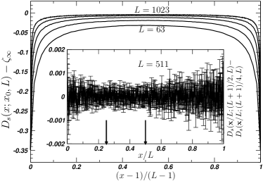
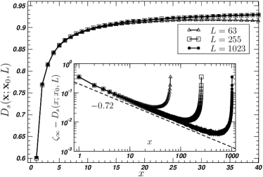
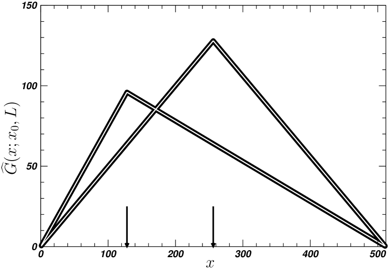
over all sites is the spatially averaged (expected) density of particles in the system at stationarity (as is taken at stationarity). As can be seen in Fig. 1(a), in large enough systems shows little variation in the bulk, as boundary effects decay, according to Fig. 1(b), independent of the system size, so that converges as for fixed and , i.e. the shoulder of , visible for small , is reproduced with increasing system size.
The inset of Fig. 1(b) suggests that the deviation of the density from the bulk value follows a power law as a function of the distance away from the boundary, , over a characteristic scale that is linear in the system size (probably related to the scaling of the correlations seen below in the inset of Fig. 2(b)). Because the amplitude of the deviation quickly converges with increasing , this is difficult to confirm in the bulk of large systems, as any deviations eventually drown in noise. This is a common theme in substrate features: Amplitudes do not display finite size scaling. The inverse of the observed exponent, should be Lübeck (2004), estimated below to be . Bonachela and Munoz have studied a range of observables in the Manna Model as a function of the distance from the boundary Bonachela and Muñoz (2007) (also Bonachela and Muñoz (2009)) and Grassberger, Dhar and Mohanty Grassberger et al. (2016) recently found the same scaling in the Oslo Model Christensen et al. (1996), which is thought to be in the same universality class Nakanishi and Sneppen (1997). They found an exponent of approximately , which is still compatible with the present data.
The density is bounded from above and from below, but nevertheless displays a small decrease with system size at the boundary sites ( and ). Because of the lack of scaling of the amplitude of the deviation, the drop in the rescaled plot Fig. 1(a) from the bulk density towards the lower density at the boundaries gets increasingly sharp with system size. For very large system sizes, the density in the bulk may therefore be approximated nearly everywhere by , Eq. (4). Numerically, the best known estimate for its value in the limit of is (Huynh et al., 2011), which our value of is compatible with. We have extracted that from our data by fitting results for against
| (5) |
which also produces a very good goodness of fit (about ) and generates, in passing, an estimate of of which compares well with previous estimates of (Lübeck, 2004).
That the density profile shows so little structure suggests that it does not even reveal the position where the driving takes place, i.e. that is independent of the driving position. Numerically, this is indeed confirmed. The inset of Fig. 1(a) shows the difference between the density profile of driven at and at . This data is fully compatible with the hypothesis that the profile does not depend on the driving position.
The stationary state, i.e. the invariant probability of finding a certain profile of immobile particles, could in principle be dependent on the way (where and how) the system is driven and also on the initialisation. For the system sizes considered here (), we do not find any such dependence. The resulting profile is independent of and other details of the driving.
In Appendix LABEL:sec:appendix_generate_matrices and more particularly Appendix LABEL:sec:appendix_eigenstates, we discuss an analytical approach to the stationary state. There, we show that in one dimension the stationary state reached by driving the Manna Model at the first site, , at the last site, , or globally with positive probability at every site (such as uniform driving), is identical and unique. This stationary state is the unique invariant distribution of configurations that is common to all driving sites. This is a remarkable feature that is in perfect agreement with the notion of self-organisation in the Manna Model, namely that there is one and only one stationary state (a distribution of configurations) that the model evolves towards, irrespective of whether it is driven at a boundary site or at all sites with positive probability.
However, as discussed in Appendix LABEL:sec:appendix_degeneracy, it turns out that the invariant probability is in fact two-fold degenerate (and can in principle be even more degenerate), as there is a conserved quantity if is odd and is even (as in the present case of odd and centre driving). This degeneracy was not picked up in the numerics mentioned above, because it is visible in the density profiles only in very small systems (see Fig. 28). For systems of size and bigger it seems numerically impossible to differentiate between the stationary states resulting from these different initial conditions and one will therefore arrive always at the (numerically) same density profile .
III.2 Correlations
In the stationary state, not only the one-point density is invariant, but in fact the probability of finding the system in any of its configurations. Indeed, the analytical results mentioned above (see Appendix LABEL:sec:appendix_eigenstates) give access also to -point correlation functions (in principle even to the response function and the “temporal shape of the avalanche” discussed below) — unfortunately, however, only for very small system sizes. These results are therefore not shown.
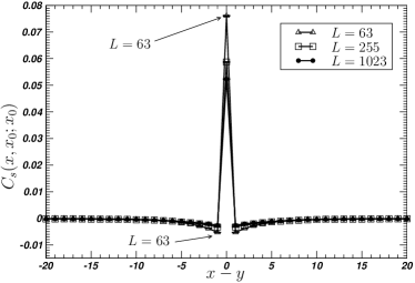
Carrying on with numerical results for systems of size , in the following we analyse two point correlations in the occupation by inactive particles. If is the joint probability of finding a particle at and another one, at the same (macroscopic, quiescent) time, at after driving at , then
| (6) |
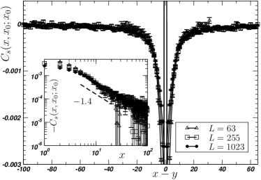
is the connected two-point correlation function. As shown in Fig. 2, small anti-correlations are present in the distribution of inactive particles. However, there is clearly no finite size scaling of the amplitude of these correlations, which cannot possibly increase indefinitely as the density is bounded everywhere. In fact, the anti-correlations die off very quickly in space. Despite being slightly less pronounced for large system sizes, they seem to converge to a finite value for increasing , i.e. they are not merely a finite size effect. Because the spatial scale of the anti-correlation does not vary significantly with the size of the system, this correlation function does not collapse under any non-trivial rescaling. However, for distances of less than about sites shows some noisy linear behaviour in a double logarithmic plot, as shown in the inset of Fig. 2(b). This may suggest a power law dependence of , albeit with a very small amplitude of about one third of the (local) variance , which is itself a small quantity (as discussed below). The power law-like behaviour persists for and, as a second moment, may be related to the exponent of found in the scaling of the deviation of the density from the bulk value, away from the boundary Fig. 1(b) and thus expected to be Lübeck (2004).
Given the small amplitude of the anti-correlations, which seems to converge from above with increasing system size, and the large relative statistical error, it is fair to say that the anti-correlations are not very pronounced and difficult to measure. There is clearly no scaling of the amplitude with system size and no rescaling needed to achieve the (noisy) collapse of Fig. 2(b). This lack of scaling is similarly found in the density profile shown in Fig. 1(b), yet the exponent roughly characterising the scaling of the correlations is about twice that characterising the decay of the density difference from the bulk value away from the boundary. Similar power law scaling is observed in in three and five dimensions (Figs. 17(b) and 23(b) respectively), but the data is obviously plagued by statistical noise. Future studies, in particular using more sophisticated observables and numerical techniques, may be more successful in identifying features in the substrate whose amplitude scales up with increasing system size and that (unlike, say, the shoulder in Fig. 1(a) localised close to boundary) remain visible even when the (apparent) lattice spacing is very small compared to the range of observation.
Within statistical error the variance coincides with the Bernoullian (which is a small quantity as is close to unity, ). To explore the correlations apparent in Fig. 2(b) further, we have also measured the distribution of distances between unoccupied sites, measured as the number of consecutively occupied sites between any two unoccupied ones. If occupation is governed by a Bernoulli process, the frequency of such distances should follow . As shown in Fig. 3, a semi-logarithmic plot produces a mixed picture. On small scales (small or small system size) significant deviations are apparent, but with increasing system size, the large scale behaviour seems to approach the expected exponential, although with a higher density of unoccupied sites (a steeper slope). Very long stretches of continually occupied sites are very rare and their statistics therefore subject to significant noise. That barely any correlations are visible on the large scale is nevertheless consistent with the observation of hyperuniformity discussed in the following.
Through a different observable, there is already clear evidence for anti-correlations in the fixed energy variant of the Manna Model, as Hexner and Levine Hexner and Levine (2015) observed hyperuniformity Torquato and Stillinger (2003) in the substrate particle density and Basu et al identified “natural long-range correlations in the background” Basu et al. (2012).
Hyperuniformity refers to the (fast) scaling of the variance of the particle density with the volume over which this density is estimated. In one dimension, the instantaneous density might be measured as a window average () symmetrically around the driving site at the centre. Its variance is given by
| (7) |
and so if sites are independently occupied. In general, if was positive everywhere, could not decay faster than . If it does, this is referred to as hyperuniformity. The variance can always be written as
| (8) |
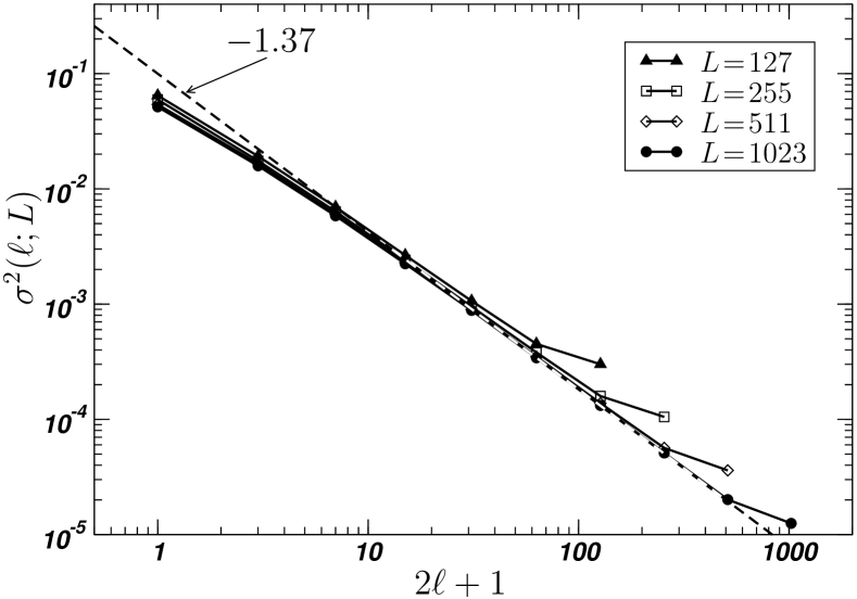
with , the correlation at , which is bound to be non-negative. At the heart of hyperuniformity is the behaviour of the sum in Eq. (8). Even if is negative for , it might still be subleading, resuling in . However, as illustrated in Fig. 4, we found a scaling of , for in an intermediate range of the width of about . We believe this value of the exponent is compatible with found by Hexner and Levine for the same quantity in the fixed energy version of the Manna Model.
Ignoring the contributions from for small or, equivalently, assuming that the positive contributions at , which scale like , are cancelled by negative ones from small, positive (where it does not follow a power law), the scaling of in large is due to the (intermediate) asymptote of , which means that the exponent of in the inset of Fig. 2(b) is to be compared to and , found for here and in Hexner and Levine (2015), respectively. Standard finite size scaling indeed suggests Grassberger et al. (2016). Notably, the scaling of , which has to be cut off when exceeds and the absence of finite size scaling of the amplitude are compatible with hyperuniformity. Our numerics indicate that the scaling of persists up to , which suggests that the scaling of is long-ranged, possibly of the form , with a cutoff length linear in the system size. Algebraic correlations of the substrate have first been observed analytically in the seminal work by Majumdar and Dhar Majumdar and Dhar (1991) on the paradigmatic Abelian Sandpile Model Bak et al. (1987); Dhar (1990) and thus may be considered the fingerprint of the critical state.
III.3 Active state
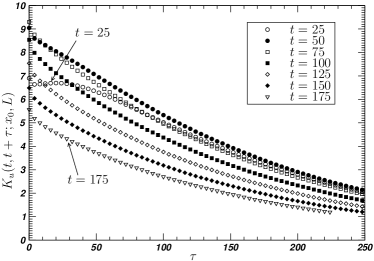
The features in the active state, i.e. during the course of an avalanche, are much richer not least due to the additional time-dependence. In the following, we will follow roughly the order of observables above. The one-point correlation function is, as above, really the response function , as defined below. It is the activity density at and (microscopic) time after the system was driven at at time . Numerically, is the estimated number of topplings of site at time after an initial charge at .
As explained above, this frequency is measured by recording the number of topplings that occur at each lattice site during the th sweep across all active sites, which is the th round of parallel updates. The zeroth sweep is the initial drive, and so at the first sweep , where is the (expected) density of particles at the driven site. In order to derive time-resolved estimates, for each time these records have to be summed over and divided by the total number of drivings. If is the record of the activity after driving attempts (macroscopic time), we use the estimator
| (9) |
from a sample of (consecutively) attempted avalanches by driving the system at site . To make the estimator well-defined for , we define whenever exceeds , the duration of the th avalanche ( if no avalanche has occurred).
The time-dependence makes the numerics more difficult to handle compared to the statistics in the quiescent state discussed above. Indeed, the response function contains more information in its space and time-dependence than, say, and even at fixed the analysis is numerically and analytically more difficult due to the additional time-dependence. To facilitate further analysis, we will focus mostly on various integrals of the response function .
By the definition of the local dynamics (toppling), the trajectories of active particles are those of random walkers. On the other hand, itself does not obey the diffusion equation,333This does not contradict the time-integrated activity, Eq. (10), to obey the Poisson equation Dhar (1990), Eq. (11). first of all because active particles may become trapped for a certain microscopic time, only to be re-activated some time later. Were those resting times discounted, each individual active particle would perform a random walk from the time it enters the system by external drive to the time when it leaves the system through an open boundary. However, regardless of how resting-times are discounted, the density is never that of pure diffusion, as there are fluctuations and correlations in the number of active particles at different times.
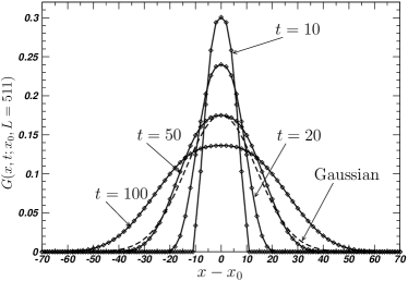
Fig. 5 shows time slices of the activity, which is, according to Fig. 5(a) almost a slowly broadening Gaussian. Below we discuss briefly in what sense a plain diffusion process is recovered, but from Fig. 5(a) it is clear that the spatial structure is not exactly but very close to a Gaussian, as demonstrated by the slight mismatch of the data (full line) and an approximated Gaussian with the same height and roughly the same width (dashed line). One may argue that the slight deviation is due to lattice effects or due to the parity conservation in the activity, as the parity of the coordinate of sites active at a given time is identical to that of . The slight difference is certainly not due to the avalanche having reached the boundaries, as times are chosen short enough.
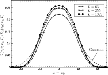
The activity also shows a mild dependence on the system size, as shown in Fig. 5(b), but seems to converge. One may think that this is due to the probability of activity being triggered at all, which is the occupation probability at the driving site, , because the (average) activity is reduced on the whole across all sites if the site driven is not occupied (and thus fails to topple). However, this is not the case, as the data in Fig. 5(b) has been rescaled accordingly. It is also not due to the avalanche having reached the boundary, as times are chosen short enough again. As the time in these figures is chosen to confine activity to the bulk, it seems most likely that the reduction of activity is caused by all sites in a smaller system having a smaller occupation probability (Fig. 1(a)), thus hindering spreading of activity somewhat. At the same time, however, stationarity is maintained, i.e. the hindrance in the activity spreading does not result in an accumulation of particles. That the time integral over all activity is nevertheless identical to that of a random walk regardless of the system size, does not mean that the activity in smaller systems, which is reduced at earlier times, must exceed that of bigger systems at later times or last longer, because the path density of random walkers increases with system size, as discussed below.
We will discuss the temporal features of the response function in further detail below. They show a very clear departure from a diffusion process, rendering the present behaviour superdiffusive.
The random walker nature of individual particles can be captured by summing over all times
| (10) |
which is the average number of topplings caused at site by driving at site . In directed sandpiles, this quantity can be used to solve the system exactly, as higher order responses can be written in terms of products of such two-point functions Dhar and Ramaswamy (1989); Dhar et al. (2015). In the stationary state, every particle added eventually leaves the system, following a random walker trajectory until it reaches the dissipative boundary. One may thus think of each particle added as producing a random walker trajectory from the source to a point at the boundary (even when the activity trace is more akin to a branching process, following individual branches of the trajectories and allowing occasional rests, produces random walker paths).
To ease notation, we adopt mostly a continuum perspective in the following. Because each toppling results in two particles being moved, the total number of topplings at site (per avalanche) is thus half the density of Brownian paths (per particle), where and is the solution of the diffusion equation, , with diffusion constant and initial condition . On a lattice is the lattice Laplacian and is to be replaced by . Carrying on in the continuum, it follows that solves the Poisson equation
| (11) |
with and Dirichlet boundary conditions identical to those on the lattice, , which in one dimension produces
| for | (12a) | ||||
| for , | (12b) |
a solution that holds identically on the lattice.
We note in passing that at half the density of walker paths is and thus clearly smaller than the response because , which means in turn that the return probability of activity is (at some later times) less than half of that of a random walker, as otherwise the time integral of activity cannot be exactly equal to half the integral over .
The Poisson equation Eq. (11) and, on the lattice, the corresponding difference equation
| (13) |
with a lattice Laplacian on the left and a Kronecker- on the right equally apply in higher dimensions. It may be interpreted and derived as a continuity equation of particles being transported from one site to another, two at each toppling. In the continuum it is easily solved in higher dimensions by
| (14) |
where are the components of in the periodic directions and is its component in the open direction, correspondingly for . The dimensional vector has components with for , whereas is a scalar with . The solution of Eq. (13) is correspondingly
| (15) |
with , , with for , and with .
The continuum solution Eq. (14) still carries the signature of the lattice: there are sites in the periodic direction with site being identical to site but only sites in the open direction, with activity on both sites and vanishing. The only quantities with the dimension of a length on the right hand side of Eq. (14) are therefore from the pre-factors and from in the denominator. Anticipating the (simplified) scaling form Eq. (25) we therefore notice that Eq. (14) can be written as with dimensionless , and . In case of the time-integrated activity, , which is a two-point response function, one can therefore identify as the correlation length analytically.
Integrating Eq. (14) over the periodic directions (sheets of constant ), as used later in Eq. (50), gives times the integrand at ,
| (16) |
and on the lattice
| (17) |
from Eq. (15), which recovers exactly Eq. (12b) with dependent on the dimension. This is not surprising as integrating over sheets of constant corresponds to considering hopping of particles only as far as their -coordinate is concerned. Given the periodicity of , the integral obeys , the differential equation in one dimension with the reduced diffusion constant of , as hops in only one of directions results in a change of sheets.
Fig. 6 confirms the triangular shape of the time-integrated activity Eq. (12b). As discussed above, the origin of the profile is somewhat trivial, but it has two important implications: Firstly, the activity is shaped by the boundaries. As opposed to the nearly featureless density profile of the inactive particles, Fig. 1, the activity is very strongly affected by the presence of the boundary, as all activity ceases there. Every particle added is eventually transported to the boundary Paczuski and Bassler (2000). Secondly, because time integrals of the response are exactly random walker profiles, the -dependence of a (suitable) propagator in a field theory will not renormalise. A non-trivial dynamical exponent , which is often obtained through the renormalisation of the diffusion constant, will have to be obtained through the renormalisation of the time-dependence. At frequency , the full propagator in a field theory reads exactly , whereas the frequency-dependence may deviate from the tree-level in almost arbitrary form, provided only that it vanishes at . Anticipating some of the discussion below, we note that the propagator being implies .
III.3.1 Spatially integrated activity
Instead of integrating the response function over time, to reduce the number of independent variables, one may just as well integrate in space. The simplest version of this quantity is the spatial integral of the activity
| (18) |
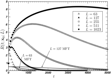
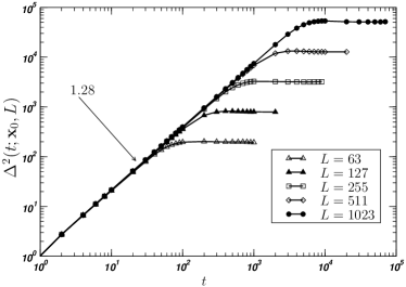
i.e. the total (spatially integrated) activity at time , which in a numerical implementation corresponds to the height of the stack of active sites with each entry being weighted by , the activity at that site. The spatial activity integral is closely related to the order parameter of many absorbing state phase transitions Lübeck (2004), the spatially averaged activity density . In fact is the area under the activity “slices” shown in Fig. 5. Numerical results, shown in Fig. 7(a), clearly differ across system sizes on the large time scale. Even on the very short time scale (, not shown separately) appears to differ systematically for all system sizes considered (although displaying some convergence). If this is solely due to the slightly decreased occupation density by inactive particles, , then the effect is cumulative and highly non-linear, as barely varies between different system sizes. For large the activity eventually reaches the boundary of the system. As is clear from the collapse in Fig. 7(b) and further discussed below, the position of the maximum total activity, , scales with the dynamical exponent, .
Employing again a continuum approximation (where we identify to ease notation), in an MFT, the spatially integrated activity is given by the propagation of the activity profile of a single active particle, which undergoes a Poissonian branching or extinction with equal rates, subject to Dirichlet boundary conditions. In one dimension the resulting profile is the spatial integral of the density , see Eqs. (16) and (17), with momenta (Pruessner, 2013), as discussed above, which gives444The integral for odd needs to be replaced by on the lattice.
| (19) |
Fig. 7(a) shows this profile as well. The mean field theory differs very clearly from the one-dimensional Manna Model in a number of points: Firstly, the tail of the mean field activity drags out for very long times, even for moderately large systems, not least as to make up for Eq. (24) below, the “sum rule” relating the mean avalanche size and the time integral over the (total) activity. In comparison, avalanches in the Manna Model are “short and sharp”. Secondly, by construction, the activity in the mean field theory never exceeds , whereas the maximum activity in the Manna Model seems to increase with system size, clearly exceeding unity even for the smallest system sizes studied. This is particularly clear at where the simple mean field assumes an activity of , whereas in the Manna Model activity is triggered with the occupation probability at the driven site.
The scaling of can be determined by making the usual (Ornstein-Zernike-like) scaling ansatz of the response Hansen and McDonald (2006); Täuber (2014),
| (20) |
where we assume, for simplicity, translational invariance, even when our systems are not translationally invariant in the -direction. Eq. (20) may be regarded of the definition of the anomalous dimension and the dynamical exponent . The dimensionless scaling function turns off correlations beyond the system size and confines them to a region of linear extent proportional to at the short time scale. Dimensional consistency is restored by metric factors and . Taking the limit in Eq. (20), the spatial integral of gives . We expect this scaling behaviour to hold for ; in fact, re-writing Eq. (20) as
| (21) |
and integrating over at finite gives
| (22) |
even for finite , or alternatively
| (23) |
with suitable metric factors and scaling function, as used in Fig. 7(b).
It turns out that in fact vanishes, as suggested in the discussion after Eq. (16). Firstly, this is implied by the sum rule arising from the temporal integral over , which is the average avalanche size,
| (24) |
written as an integral for convenience. In the present case of centre driving, the average avalanche size scales in like and follows from using the scaling form Eq. (23) in the integrand of Eq. (24).
A more subtle demonstration that follows from the time integral of the activity, which reduces the activity to random walker trajectories. Taking the time integral of Eq. (20) gives
| (25) |
with a new, suitably defined scaling function . This observable, , is the average number of topplings at site per particle added at site , as discussed at the beginning of Sec. LABEL:sec:active_state_1D, see Eq. (10). An Ornstein-Zernike correlation function Hansen and McDonald (2006), as the one generated by the density of Brownian paths has and must coincide with Eq. (25), so follows. Alternatively, one may consult in Eq. (12b) and Eq. (14), which indeed behave like for fixed .
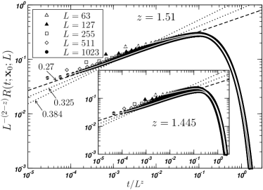
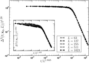
Taking henceforth, Fig. 7(b) shows a good collapse on the basis of Eq. (23) with , in poor agreement with the literature value of based on the scaling of avalanche durations Huynh et al. (2011). The collapse based on is shown in the inset of Fig. 7(b). White lines for the data of and have been added on top of the symbols to assess the quality of the collapse, which, away from the tail, is clearly worse for than for .
Apart from the collapse in , according to Eq. (22), there is also scaling in at large enough but early times. Clearly, for fixed the total activity converges in large , as for sufficiently large the activity no longer reaches the boundaries, which therefore become irrelevant. Apart from small (but possibly cumulative) effects due to the density of inactive particles, for fixed a regime exists where independent of (large) , so that in Eq. (22), which carries all -dependence, is constant, or equivalently, that in Eq. (23) behaves like a power law itself, . Therefore in Eq. (22) shapes on the short time scale, and the scaling function on the long time scale.
The initial power law regime is clearly visible in Fig. 7(b), which suggests and thus , again quite off the expected value of from (Huynh et al., 2011), also shown in the plot. A third slope shown in Fig. 7(b), is determined by giving the best collapse, . However, measuring exponents by fitting a section of the data against a straight line in a double logarithmic plot ignores the rôle of the scaling function and is generally prone to errors (Clauset et al., 2009; Deluca and Corral, 2013; Christensen et al., 2008). The significance of the slopes shown in Fig. 7(b) is therefore that both slopes of and (corresponding to and respectively) seem to be consistent with the data, whereas the literature value of fails, producing a slope of , which is clearly off.
III.3.2 Temporal shape of the avalanche
The Manna Model differs from the MFT above in that particles and thus activity display some complicated “resting”, but otherwise trajectories are random walks. Time integrals over the activity therefore remove any non-trivial behaviour, whereas space integrals retain it. It is thus worthwhile to look for ways of extracting universal features from or similar quantities.
Because is bound to scale in order to accommodate the average avalanche size, no convergence of can be expected in large at large . To observe convergence for all , the profile has to be rescaled by the duration of the avalanche and the mean activity. Theory has access (at least at MFT level) to an approximation of the spatial integral of the activity conditional to a certain time of termination, , the duration of the avalanche, but it is difficult to condition in addition to a certain avalanche size. Numerically, on the other hand, this would be trivial: If is an individual measurement of the space-integrated activity at time of an avalanche that has size and duration , then would be the relevant quantity to consider. Instead we note that
| (26) |
is the avalanche size if is the duration and averaging over the rescaled measurements ,
gives , so that normalising by (the estimate of) produces
| (27) |
a quantity that has a unit-integral and may therefore be expected to converge. Closely related to this is a quantity sometimes referred to as the “temporal shape of the avalanche” (Le Doussal and Wiese, 2013; Thiery et al., 2015), first studied by Kuntz and Sethna Kuntz and Sethna (2000) (see also Baldassarri et al. (2003)), and closely connected to the () power spectrum Laurson et al. (2005). To make in Eq. (27) well-defined in case of (and thus ), one may consider the above derivation with replaced by and take the limit .
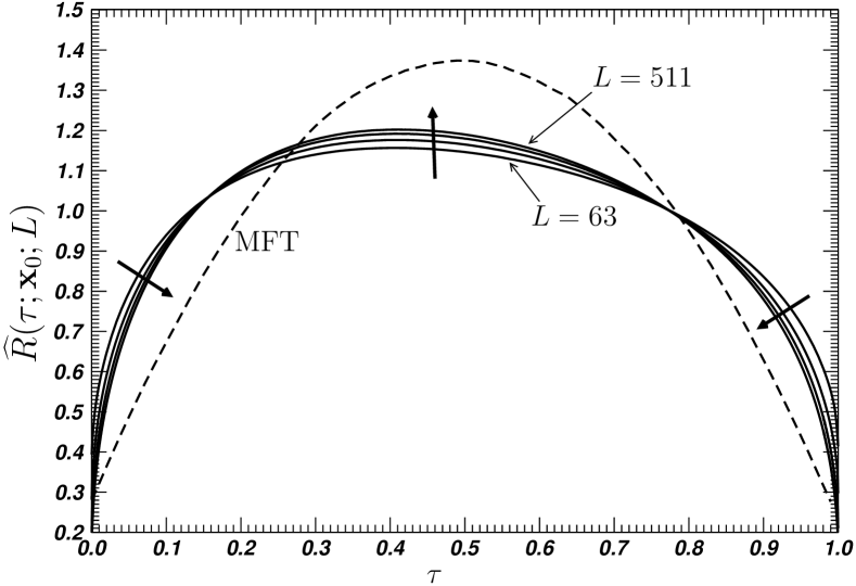
Fig. 8 shows for different system sizes , demonstrating the expected convergence. Notably, the graph displays a slight, unexpected asymmetry that is absent in the mean-field theory of a branching process.
Because the time averaged total activity diverges (slowly) for and at is exactly the finite occupation density at and expected to be small at , in the thermodynamic limit, is expected to vanish at and (and one may speculate that the MFT gives asymptotically ). In a suitable theory, one may redefine time and observables such that is exactly unity at these points.
III.3.3 Width of the response
In the following we want to characterise further the deviation of the activity density from plain diffusion. In Fig. 5 we have demonstrated that the spatial distribution of activity at in response to driving at at is very close to Gaussian. We may proceed by determining the kurtosis etc, but as mentioned above, it is difficult to attribute any deviation correctly, because there are several sources for corrections: finiteness of the lattice, boundaries, discretisation in space, discretisation in time and separation into even and odd sublattices. Only the time integral of the activity can be mapped exactly to a random walk, which is approximated by a Gaussian in the continuum. It turns out that the temporal evolution of the spatial distribution of activity is strongly superdiffusive. To see this more clearly, we may calculate the spatial variance of the normalised , using the spatial integral , Eq. (18). The width of the response may be defined as
| (28) |
In the present definition, looks very much like a mean squared displacement, except that many particles contribute to simultaneously and only very few have actually been displaced starting from , the origin. In fact, many may have been moved towards and most may have moved only a couple of sites.
Fig. 9(a) shows a very clear power law dependence of on (small) time , scaling faster than linear in for intermediate times (below a cutoff set by the system size), thus rendering the process superdiffusive. To relate this to the results above, we integrate using Eq. (21) over , which gives
| (29) |
using Eq. (22), regardless of .
If (expected for but not guaranteed as the scaling function may contribute, Eq. (29)), Fig. 9(a) suggests and thus rather than of Huynh et al. (2011). This is confirmed by a collapse, Fig. 9(b). The value of from the -dependence of is reasonably consistent with the value of from the -dependence of in Fig. 7(b) (). The literature value of produces a rather dissatisfying collapse shown in the inset of Fig. 9(b), that improves in the tail (large ) only because converges to and so plotted versus produces a straight line in a double logarithmic plot with slope for any . We will discuss the range of results for further in Sec. LABEL:sec:conclusion.
III.3.4 Further spatial scaling of the response
A quantitative test for scaling is to extract “moments” by integrating out all but one independent variable. This procedure leads to the measurements normally taken in SOC De Menech et al. (1998), such as moments of the avalanche size (for example, the temporal integral of gives ). The usual caveats apply, in particular finite size corrections, which we have largely ignored in the present analysis. A qualitative test of scaling is to attempt a collapse of the data, such as the one for in Fig. 7(b). However, for this is difficult to attain in the form (20) as there are at least three independent parameters, (assuming translational invariance), and , listed in order of increasing sparseness. In principle such a collapse can be done in three-dimensional plots, but the small range of compared to the high density of points in and the still fairly large range and number of measurements in , makes it difficult to assess the quality of such a collapse, which becomes nearly useless when projected into two dimensions.
To investigate further the spatial dependence of the activity , we consider fixed , so that according to Eq. (20) with ,
| (30) |
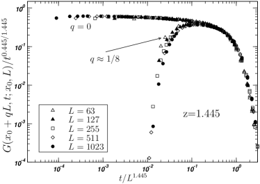
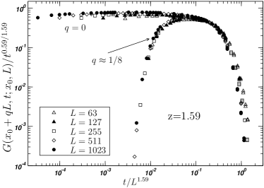
which for fixed ought to collapse when plotting against (for the earliest to the latest times ). Fig. 10 shows a collapse for () as well as () with centre driving, . While the literature value of works fairly well, Fig. 10(a), the collapse is relatively insensitive against different choices of the dynamical exponent ( is shown in Fig. 10(b), exceeding even above, see Fig. 7(b), but identical to the used in Fig. 11).
Assuming instead produces a collapse of on the basis of Eq. (20) when plotting against for different and , Fig. 11. The main panel shows a fairly neat collapse in the tail, while the inset shows a somewhat broader tail which, however, seems to cover a wider range of data, incorporating even the data marked by “off”. Picking, however, the data as to exclude those that do not produce a collapse, presumably on the basis that is violated, is a form of biased selection.
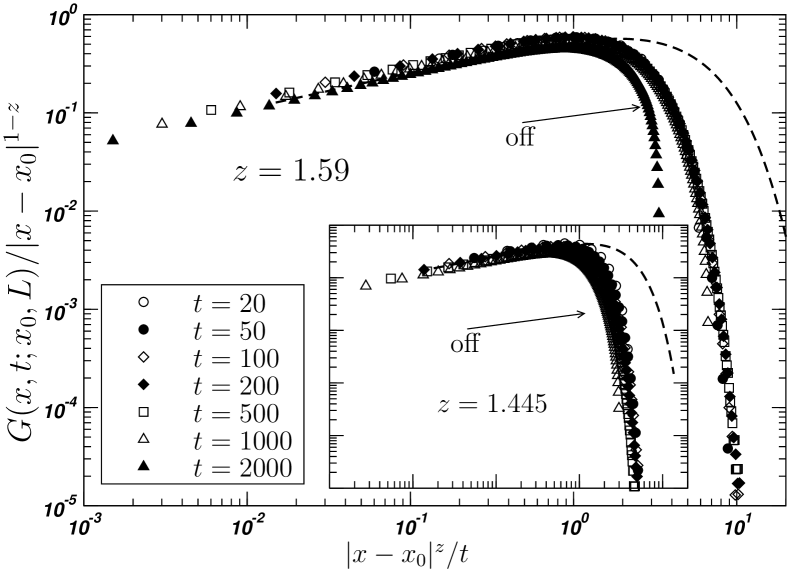
In summary, the scaling of the response is exactly as expected in a critical finite system: on the short time scale the characteristic length is set by the time , Eqs. (20) and (22) (demonstrated in Fig. 7(b)), and on the long time scale by the system size in the form , as discussed in Sec. LABEL:sec:shape_of_ava_1D (Eq. (22) and discussion towards the end). Indeed, with the time-dependence integrated out, activity has all characteristics of a random walk (Fig. 6), so that all the non-trivial features are to be found in the time-dependence. While collapses such as Fig. 7(b) and Fig. 9 confirm the presence of scaling, the exponent we found in one dimension varied: In Fig. 7(b) from the collapse but from the scaling in of , in Fig. 9(a) from the collapse and the scaling in of the width and in Fig. 10 no clear outcome ( but also ) for the scaling of the activity . On the other hand, the dynamical exponent determined in the literature from the scaling of the cutoff of the avalanche duration is Huynh et al. (2011). We will discuss this discrepancy further in Sec. LABEL:sec:conclusion.
III.3.5 Activity-activity correlations
There are very little spatial correlations in the density of the inactive particles (Fig. 2). This is very different for the activity. The correlation function to be considered next is, strictly speaking, a three-point function, as it measures the correlations of activity at different sites and in a system driven at . Although we have also considered data where all three sites are distinct, generally statistics is better for (or , which amounts to the same), so we have focused on that case.
This correlation function is also a function of two times relative to the time of driving. We decided to consider only equal time correlations, with the aim to extract interesting spatial behaviour. The estimators for the unconnected activity-activity correlation function
| (31) |
and the connected correlation function
| (32) |
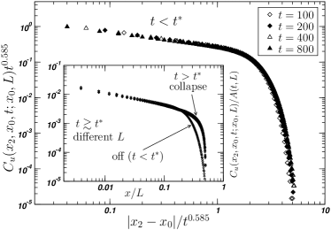
are based on the same measurements of local activity as Eq. (9). Choosing still leaves us with four independent variables. To capture the temporal evolution, we chose to take samples only at for a range of different system sizes, all driven at the centre. However, as mentioned in Sec. LABEL:sec:observables, activity vanishes on sites whose distance to the driven site has a parity different from that of , and in particular strictly for all at odd , so that both and vanish at odd . From the data shown in Fig. 12(a), it is clear that the unconnected correlation function collapses in one dimension for different, early according to
| (33) |
with some amplitude , exponent (here similar to the exponent in Eq. (39) below, whereas (Huynh et al., 2011)) and scaling function , but “saturates” for like (inset of Fig. 12(a))
| (34) |
where is no longer a power-law in (as effectively in (33)), but is instead dominated by an exponential in . For fixed , that amplitude is essentially the fraction of “survivors”, i.e. the probability of an avalanche lasting at least until . Data for is shown in the inset of Fig. 12(a), together with data of the correlation function not quite at saturation (labelled “off” as opposed to “collapse”). The evolution of the activity-activity correlation function is therefore compatible with the classic narrative of correlations spreading throughout the system as the avalanche unfolds Grinstein (1995); Dickman et al. (1998); Lise (2002), until the effective correlation length (the cutoff length in Eq. (33)) reaches the boundaries, suggesting (see below). For essentially all the time thereafter and thus most of the time, the correlation function has the form (34), although numerical data for very long times becomes very noisy.
We are unable to offer an explanation for the scaling form Eq. (33), because of the many different variables and scales involved. It depends on at least two different points in space and on a time that needs to be small enough so that Eq. (33) applies, determining implicitly. The most striking feature of the scaling form is that the exponent in the pre-factor is identical to the exponent in the argument of the scaling function, which we expect to be . However, (based on in Fig. 12(a)) is greater than any measured above. Below we will derive the scaling of the time-averaged correlation function , but it is difficult to relate it to the scaling of (33), as the latter requires .
Repeating the analysis for the connected correlation function , Eq. (32), shows rather poor collapses. It remains somewhat unclear why that happens. The second term in (32) has a fairly small contribution, yet big enough to spoil most collapses. A collapse like Fig. 12(a) for is rather noisy and dissatisfying, producing no reasonable estimate of according to Eq. (33).
If the activity correlations can be regarded as “almost stationary” (or quasi-stationary as in fixed energy sandpiles Dickman et al. (1998); Vespignani et al. (1998); Lübeck (2004)), it is justified to take their time average. If is the duration of the th avalanche, then
| (35) |
estimates the time-averaged activity at site conditional to activity (somewhere) Pruessner (2007), as otherwise time stops passing. Because , the time-average is the average number of topplings of site per avalanche, i.e.
| (36) |
see Eqs. (9) and (10). Correspondingly, the unconnected time-averaged correlation function may be written as
| (37) |
and the connected one as
| (38) |
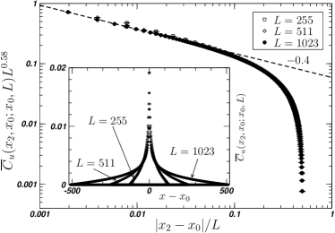
The unconnected time-averaged correlation function for (in one dimension) is shown in Fig. 12(b) and displays a remarkably good collapse
| (39) |
for different system sizes with (for an earlier estimate of based on uniform driving see McAteer et al. (2016)). The denominator in the argument of the scaling function should be regarded as the correlation length, which is in fact proportional to the system size, exactly as expected for a finite system at the critical point Bak et al. (1987, 1988); Lübeck (2004); Pruessner (2012); Watkins et al. (2016). The exponent that scales the amplitude in Eq. (39) can be related via a sum-rule to known scaling exponents, such as the scaling of the activity variance (Lübeck, 2004; McAteer et al., 2016) (see Eq. (2.36) in Lübeck (2004), is the variance of the density and is the spatial integral of the variance),
| (40) |
where we have used the notation of Lübeck (2004), except that we use for the spatial dimension (denoted by in Lübeck (2004)). If the scaling of is essentially translationally invariant, as suggested in Eq. (39), then from Eq. (40) and thus . The estimate above (Fig. 12(b)) is perfectly in line with literature values of in one dimension Lübeck (2004).
Alternatively, one may relate to the second moment of the avalanche size. Given that the instantaneous avalanche size is Eq. (26), the estimator for the second moment is exactly equivalent to
| (41) |
resulting in a corresponding sum rule on the unconnected correlation function. It requires, however, the two (three) point, two time correlation function. Assuming that it follows essentially Eq. (39) with and as additional arguments in the scaling function, gives
| (42) |
where undoes the normalisation in Eq. (37) compared to Eq. (41), is due to the double space integral (or sum, Eq. (41)), is due to the additional time integral in Eq. (41) compared to Eq. (37) and, finally, is due to Eq. (39). Given that , and (all exponents explained in detail in Pruessner (2012)), one arrives at which is in line with because what is denoted here is in Lübeck (2004) and so here is in fact there. However, gives using the values of and of Huynh et al. (2011). The mismatch with mentioned above cannot be explained by the dynamical exponent of measured in Lübeck (2004), which gives an even smaller value of . Rather, it is the poor match of in Lübeck (2004), which gives based on measurements in the fixed energy sandpile (FES) version of the Manna Model, and of Huynh et al. (2011) taken in the SOC mode.
The slope of , Eq. (39), that is so clearly visible in Fig. 12(b) (dashed line) may be captured by fitting against a power law with a cutoff, so that for small . For sufficiently small and sufficiently large , the correlation function thus behaves like . It is difficult to see how to relate this behaviour to known exponents through scaling relations.
The connected time-averaged correlation function collapses as well, but is much less sensitive to a change of the exponent in Eq. (39). While it is compatible to , with some small deviations, its tail ( close to unity) still collapses even for . That the tail collapses so easily is of course unsurprising, as vanishes as sites become uncorrelated, i.e. when approaches , and a sharp drop is very insensitive to rescaling.
III.3.6 Two-time activity correlations and -noise
Historically, SOC was introduced as an “explanation for noise” Bak et al. (1987), even when that notion quickly took a less prominent place Pruessner (2012); Watkins et al. (2016). The initial measurement Bak et al. (1987) of the power-law characteristics of the power spectrum of the BTW Model was soon revised by Jensen et al Jensen et al. (1989), who had to made a number of drastic assumptions in order to link the power spectrum to the avalanche duration distribution. A more recent, detailed numerical analysis by Laurson et al Laurson et al. (2005) found non-trivial noise in both the BTW and the Manna Model.
In the following, we analyse the correlations in the spatially integrated activity signal
| (43) |
of avalanche with duration , which, of course, varies among avalanches. That makes the calculation of correlations somewhat ambiguous,555Apart from allowing for vanishing (see below), one may, for example, rescale time to the unit interval or weight avalanches of different durations differently. in particular when taking averages over ensembles. We intend to carry out the following analysis in the spirit of the original link of SOC and spectra. To arrive at a single time series, we effectively concatenate consecutive by inserting an infinite trail of zeros.
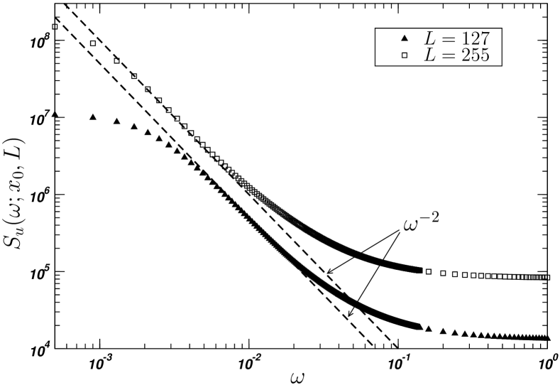
We will make use of the estimators (cf. Eqs. (31) and (32))
| (44) |
and
| (45) |
where the second term makes use of , which is the expectation of , Eqs. (9) and (18). To make well-defined for all , we take for . This together with Eq. (44) that never mixes different avalanches, amounts to analysing correlations in concatenated activity histories as if each was succeeded by an infinite trail of zeros, thereby implementing separation of time scales. Other choices have been made in the literature, notably by Laurson et al who suggest the effect of trailing zeros is negligible Laurson et al. (2005).
As the process is not time-homogeneous, are functions of two times and . In the past, this feature was to large extent ignored. In Jensen et al. (1989) the authors assume that is a top-hat function with duration and height , approximating by a suitably weighted integral of convolutions of that top-hat.
From Fig. 7 it is clear that in the Manna Model, is not overly well approximated by a top-hat. In the following, we want to explore the shape of the unconnected and connected correlation functions and . The first question that arises is whether it is justified to assume that and are essentially functions of the time lag , but otherwise independent of . Fig. 13(a) shows that this is indeed the case for a range of at least as far as the connected correlation function is concerned. This feature is clearly less pronounced for the unconnected correlation function, Fig. 13(b), which, however, is closer to the one studied in the past with regard to its characteristics in the BTW Model Jensen et al. (1989); Laurson et al. (2005).
Carrying on along the lines of Jensen et al Jensen et al. (1989) but also Laurson et al Laurson et al. (2005), the unconnected two-time correlation function is time-integrated (not time-averaged, as usual, e.g. Gardiner (1997)) over ,
| (46) |
and Fourier-transformed,
| (47) |
which resembles a sigmoidal shape, as shown in Fig. 14, quite different to what Laurson et al Laurson et al. (2005) obtain using a different concatenation scheme. The intermediate drop may be approximated by a power law, , consistent with similar findings in the BTW Model Jensen et al. (1989), but it is difficult to trace that behaviour back to the decay of temporal correlations.
In fact, there is little non-trivial, asymptotic long-time behaviour in or at all. What displays scaling in these quantities is their cutoff (because of the scaling of durations), but not the correlation functions themselves, Fig. 13(a). The approach by Laurson et al Laurson et al. (2005) has clearly been more successful in that respect.
One might be tempted to repeat the above analysis for the connected correlation function as defined in Eq. (45). However, taking an average like Eq. (46) over the unconnected part remains ambiguous. It is arguably to be replaced by the square of the average activity , in which case, however, the time averaged no longer drops to for as normally expected for a connected correlation function. Given that our main interest in the present correlation functions was to make contact with the historic research focus, namely -noise as studied in Jensen et al. (1989), we did not pursue this approach any further.
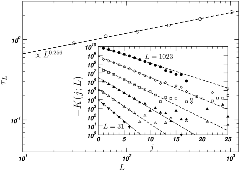
III.3.7 Macroscopic time correlations
We finally consider the correlations in the size of consecutive avalanches, as a function of , estimated via Anderson (1971)
| (48) |
In the Oslo Model Christensen et al. (1996) the avalanche size can be interpreted as the displacement of an interface pulled on one end over a rough surface Paczuski and Boettcher (1996); Pruessner (2003, 2012) and the macroscopic correlation time is, in this model, therefore related to the interface’s roughness, which scales like with . In the present case, neither the mapping exists nor can the driving be interpreted easily as a pulling force. Following nevertheless the same argument as in Paczuski and Boettcher (1996), the typical total number of topplings needed to avoid an overlap between initial and final interface configuration scales like . The number of avalanches to be triggered to reach essentially independence is therefore of order , which in the present case scales like as , Eq. (1) with . In other words, the macroscopic correlation time should scale like Huynh et al. (2011).
It is difficult to extract good estimates of the macroscopic correlation time from the data. As observed in directed models Welinder et al. (2007), correlations for are anti-correlations, , as large avalanches are normally followed by smaller ones and vice versa. Fig. 15 shows in a semi-logarithmic plot in the inset, suggesting an exponential decay of correlations, which are quite short-lived in one dimension (and obviously orders of magnitude shorter than the transient). Fitting them (by eye), with amplitude , and plotting the resulting estimates for the correlation times yields a scaling of approximately , as shown in Fig. 15, compatible with quoted above.
IV Higher dimensions
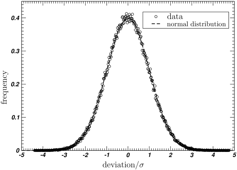
We have repeated many of the measurements discussed above in three and five dimensions. Because the upper critical dimension of the Manna Model is Lübeck and Hucht (2002); Lübeck and Heger (2003a); Lübeck (2004), is expected to be much closer to mean-field results (and in that sense better behaved), whereas is expected to reproduce them at least as far as universal quantities are concerned.
As the most interesting observables to consider in higher dimensions, we have selected the density of inactive particles in the quiescent state (cf. Sec. LABEL:sec:quiescent_state_1D), the spatially integrated activity (cf. Sec. LABEL:sec:shape_of_ava_1D), the temporal shape of the avalanche (cf. Sec. LABEL:sec:temp_shape_of_ava), the width of the response (cf. Sec. LABEL:sec:msd_1D), the spatial activity-activity correlation function (cf. Sec. LABEL:sec:actact_corrs_1D), and the macroscopic time avalanche-avalanche correlations (cf. Sec. LABEL:sec:ava_ava_corr).
Numerically, dimensions greater than one pose the disadvantage of high memory requirements for comparatively “small” system sizes as far as linear extent is concerned. In particular in five dimensions, lattices of linear extent beyond are difficult to realise. The largest lattice we used in five dimensions therefore was . We have avoided scanning lattices as much as possible (see discussion before Eq. (3)), so that CPU-time requirements are mostly determined by the average avalanche size . The largest lattice in three dimensions was . As discussed above, periodic boundary conditions were applied in all but one (open) direction.
The periodic boundary conditions may suggest that observables do not depend on the coordinates orthogonal to the open direction (parameterised by ). We will indeed consider in the following certain observables with respect to their sheet-average (spatial average at constant ) and their deviation from it. Yet, given centre driving at one single site , , translational invariance is broken in every direction.666If one is not interested in the particular symmetries of the system, this can be cured by driving (randomly) across entire sheets of constant . This is expected to be reflected in the observables, for example the response function: Periodic boundary conditions or not, activity that begins in a point will not spread instantaneously across entire sheets of constant (which are of size ).
IV.1 Three dimensions
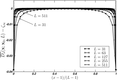
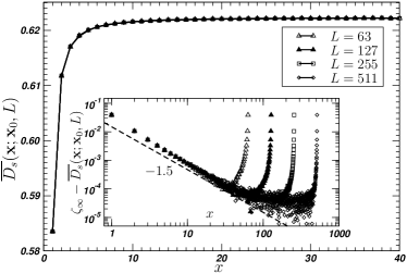
It turns out, however, that even with (non-translational invariant) centre driving the density of inactive particles displays translational invariance within sheets of constant . It is rather futile to attempt to visualise that by plotting the density profile for constant (coordinates within a sheet). Fig. 16 shows instead a histogram of the number of standard deviations by which the (estimated) density at each and every point within the sheets deviates from the average within a sheet,
| (49) |
where . The result is a distribution very close to a normal distribution (also shown), suggesting that the small deviations of local densities from the sheet average are possibly random and independent rather than systematic. However, confirming that by direct measurements of correlations is difficult, firstly because of the statistical noise (as seen in Fig. 2(b)) and secondly because of the wide range of correlations to consider. For example the two point function , Eq. (6), depends on the positions relative to the open ends, and , as well as the displacements in the periodic direction, . Again, integrated observables, such as the window-averaged density Eq. (7), might be better suited to reveal (anti-) correlations.
Given the (observed) translational invariance in the periodic directions, Fig. 17 shows the sheet-averaged density profile across the open direction in three-dimensional systems as the deviation from the bulk value Huynh and Pruessner (2012). This data shows little qualitative difference compared to Fig. 1, except that the density remains much closer to the bulk value throughout, even close to the boundaries and even for comparatively small systems. The range of the ordinate of Fig. 17(a) is about an order of magnitude smaller than in one dimension. Fig. 17(b) shows that the profile close to the boundary displays no discernible difference among the system sizes considered; there is certainly no finite size scaling of the amplitude of the profile. However, similar to one dimension, Fig. 1, boundary effects decay like a power law. We estimate the exponent to be around (as shown in the inset of Fig. 17(b)), but a reliable estimate is hampered by the high level of noise in the data and does not improve much when the data is binned. For comparison (see discussion in Sec. LABEL:sec:quiescent_state_1D) Lübeck (2004), compatible with the exponent estimated here.
Integrating the local activity over the entire lattice produces the total activity, , as defined in Eq. (18). As discussed in Sec. LABEL:sec:shape_of_ava_1D, we expect plotting against to produce a collapse. In dimensions this is indeed the case and works very well using , based on the dynamical exponent as obtained in Huynh and Pruessner (2012); Fig. 18 shows a corresponding collapse like the one obtained in Fig. 7(b) in dimensions.
Also shown in this figure is the slope of the rescaled total activity in rescaled time, which we expected to display an exponent of (see the discussion in Sec. LABEL:sec:shape_of_ava_1D). While this was not fully confirmed in one dimension, it is perfectly in line with the findings in three dimensions.
Normalising the activity profile in the form introduced in Eq. (27) produces the “temporal shape of the avalanche” shown in Fig. 19 together with the mean field theory introduced in Sec. LABEL:sec:shape_of_ava_1D and Sec. LABEL:sec:temp_shape_of_ava. The curves are remarkably close given that the mean field theory should apply only in dimensions of . The data still shows a slight skew which is difficult to see by naked eye. The mean field data displays a similar slant (possibly a finite size effect), but in the opposite direction. The collapse thus improves when plotting against the MFT.
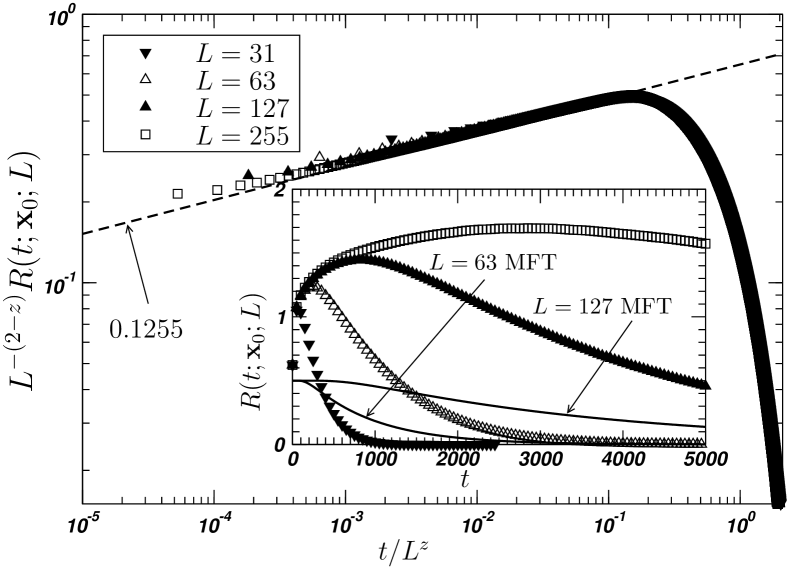
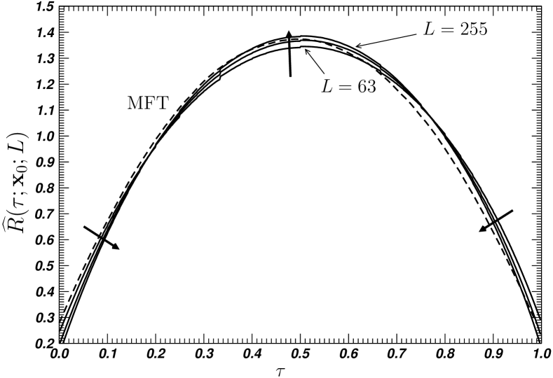
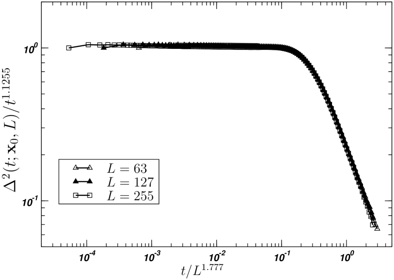
The width of the response propagator, , as defined in Eq. (28) produces a collapse if rescaled suitably, as shown for in Fig. 9(a). In Sec. LABEL:sec:msd_1D it was demonstrated that in one dimension the collapse requires a dynamical exponent, , that deviates quite clearly from the expected value of from the literature. In Fig. 20 we show that the data in three dimensions is compatible with the expected value, Huynh and Pruessner (2012), apparently validating the scaling arguments in Sec. LABEL:sec:msd_1D. The possible causes of the mismatch in one dimension is discussed further in Sec. LABEL:sec:conclusion.
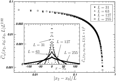

As mentioned above, the propagation of activity (the response function) is certainly not expected to be translationally invariant, as activity surely is correlated to the position of the initial driving. However, it is numerically very challenging to analyse spatial data as a function of all components. We have therefore decided to study activity and its correlations after spatially averaging in the periodic direction. This way we obtain enough statistics and yet can still test for the expected scaling behaviour.
As indicated in Eqs. (16) and (17), averaging (or, for that purpose, summing) the time-integrated activity over the periodic direction reproduces the one-dimensional profile Eq. (12b). The resulting profiles of the time-integrated activity summed over the periodic direction look therefore up to a pre-factor exactly like Fig. 6.
Activity-activity correlations on the other hand show some clear non-trivial scaling as a function of space. Defining the time-integrated, sheet-averaged activity in terms of the numerical observable as
| (50) |
produces a function of essentially only one variable, , the position in the open direction with the shape shown in Fig. 6, see Eq. (17). The activity-activity correlation functions may be defined in the same vein,
| (51) |
and
| (52) |
with and . Noticeably, and have each dashed components which are summed over independently, with the intention to render correlation functions of spatial averages rather than spatially averaged correlation functions. This is a matter of choice, motivated by the independence of the two coordinates in Eq. (40).
Both correlation functions collapse very nicely under suitable rescaling, similar to Fig. 12(b). Fig. 21 shows the collapses by plotting against , Eq. (39), with for the unconnected correlation function and for . Just like in one dimension, we have chosen , i.e. one sheet in the two-point correlation function is the one where the driving takes place. The exponent should be compared to from Lübeck (2004) or Huynh and Pruessner (2012), see the discussion after Eq. (39). These two values from scaling relations do not fully agree, but not as significantly as in one dimension, where they suggest and respectively. Moreover, the collapses with and are relatively better compatible with these literature values in both cases (in contrast to in one dimension, which is much less compatible with than with ). One may wonder that the unexpectedly inconsistent scaling is a feature of one dimension (see also Lübeck and Heger (2003b)).
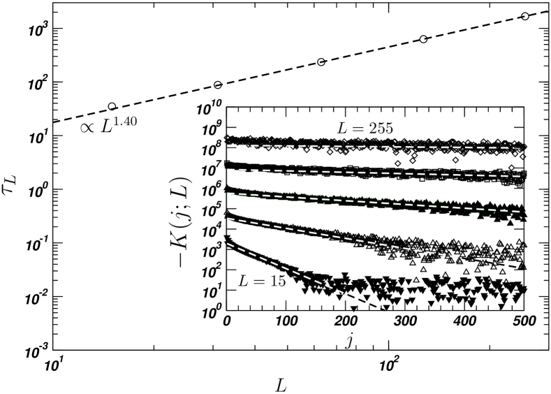
Finally we consider correlations of avalanche sizes on the macroscopic time scale. Compared to one dimension, where correlation “times” (measured in number of avalanches attempted) are fairly short and do not increase dramatically with system size, correlations in three dimensions last much longer and rise significantly. Fig. 22 shows the correlation function (in the inset, Eq. (48)) and the estimated correlation times, which change from around avalanches at to about avalanches at . Fitting the correlation time against the system size results in an exponent of , which is not too far off the expected value of Huynh and Pruessner (2012) (see discussion after Eq. (48)).
IV.2 Five dimensions
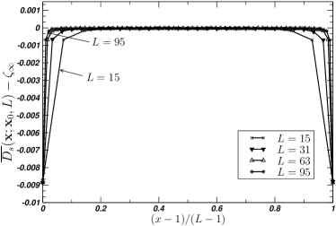
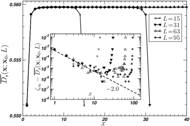
Five dimensions are supposedly above the upper critical dimension and so the Manna Model should display the same asymptotes and, in particular, the same scaling, as its Mean Field Theory Le Doussal et al. (2016), where and Lübeck (2004). Because of the high dimensionality, the linear extent of the systems studied numerically is rather limited. The largest lattice we used was thus with sites. With a particle density of that means one cannot reasonably expect the system to equilibrate within avalanches when starting from an empty lattice. For these very large systems, we decided to determine the bulk density on a smaller lattice (starting from , having sites) over the course of avalanches, and use that density uniformly as the initialisation for the next bigger lattice. In each case, we dismissed avalanches as transient.
As seen already in the sharpening of the density profile from one dimension, Fig. 1, to three dimensions, Fig. 17, in five dimensions, Fig. 23, the density across different four-dimensional sheets of constant is nearly the same everywhere in the system. Only around and a deviation from the bulk density is actually noticeable but still is minute. To determine , we have fitted against with fitting parameters , and . From we found (and ) with a goodness of fit of , which is to some extent owed to the small number of data points and the comparatively large number of fitting parameters. In the inset of Fig. 23(b) we used instead, as it produced a more systematic dependence of the apparent cutoff on the system size. In that figure, we show that the small deviations of the substrate density from the bulk value close to the boundaries is reproduced for different system sizes and may display some power law dependence on the distance (similar to Figs. 1(b) and 17(b)). Unfortunately the data is too noisy to extract a reliable estimate of the exponent. Fig. 23(b) shows exponent for comparison.
While the particle density is non-universal and difficult to capture theoretically, the total activity , Eq. (18) (Sec. LABEL:sec:shape_of_ava_1D), as shown in Fig. 24 and its normalised form , Eq. (27) (Sec. LABEL:sec:temp_shape_of_ava), as shown in Fig. 25, display universal scaling, as shown in Figs. 7(b) and 8, in one dimension and in Figs. 18 and 19 in three dimensions. The former, , is based on the collapse of the rescaled activity as a function of suitably rescaled time, the latter, on the universal shape of the activity profile averaged after scaling it to the interval .
Fig. 24 shows the activity as a function of rescaled time using the exponent , Eq. (23). Indeed, no initial slope is visible in , as expected for , Eq. (22) (see Sec. LABEL:sec:shape_of_ava_1D). Accordingly, the collapse occurs when time is rescaled by . The inset shows a comparison to the MFT as introduced in Sec. LABEL:sec:mft. While the match is far from perfect, it shows a noticeable improvement over the data for , Fig. 18, and the data for , Fig. 7. It could surely be improved further by rescaling the activity so that it matches, initially, the density of immobile particles, , as the activity at is exactly the probability of the initial particle (supplied by the external drive) arriving at an occupied site. A qualitative difference to the situation in and (Fig. 18 and Fig. 7(a) respectively) is the fact that the activity drops almost monotonically, apart from a very slight initial increase. In and it shows a very clear maximum, that exceeds unity in both cases.
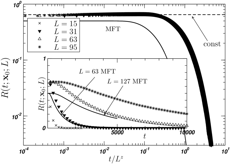
Fig. 25 shows a comparison of the (specially normalised) activity profile according to Eq. (27) and the profile expected from mean field theory, i.e. the branching random walk (Sec. LABEL:sec:shape_of_ava_1D), which are expected to share the same universal shape. The data for the five-dimensional lattice is in good agreement with the MFT. Because of the large avalanche duration exponent and avalanche size exponent Pruessner (2012) in five dimensions, relatively many avalanches are short in time and small in size, so that the data used for in Eq. (27) is mostly rather stepped. That results in visible artefacts as seen in Fig. 25, made worse by the fact that the artefacts align for different system sizes. The situation can be improved by using Poissonian updating which smears out the steps or by introducing a cutoff to suppress avalanches below a certain size.
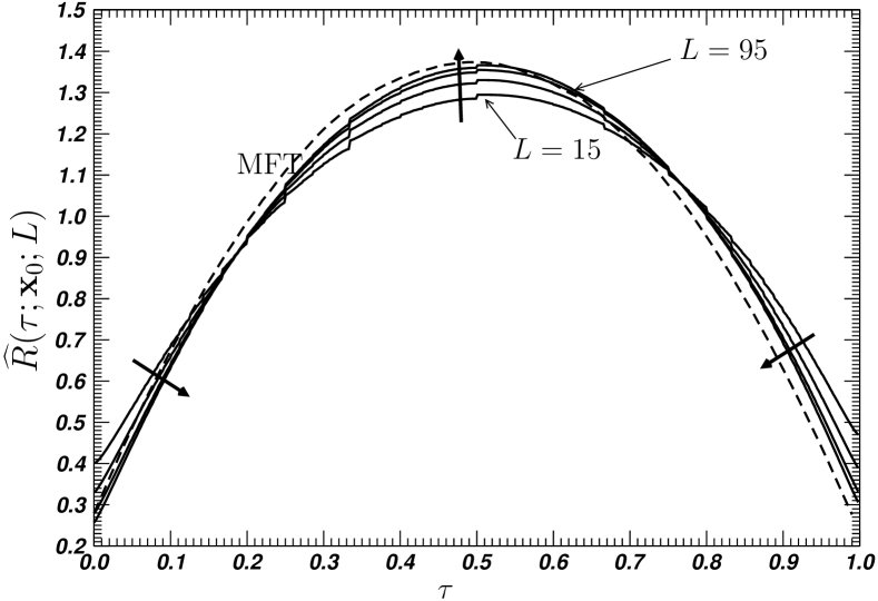
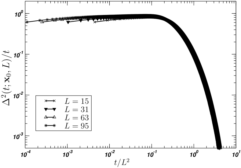
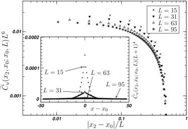
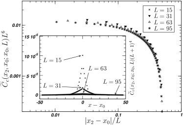
Comparing the data in Fig. 25 to that in Fig. 19 suggests that the mean-field theory works better or applies at least as well in three dimensions as in five. One possible explanation is that system sizes in five dimensions are much smaller and so the coincidence between mean field theory and data in five dimensions would actually be significantly better, if bigger system sizes were available. Inspecting the data in Fig. 19 suggests that the data may display convergence away from the mean-field curve, whereas the data in Fig. 25 is still compatible with a convergence towards it. However, even the mean-field data is based on a comparatively small lattice (, see Sec. LABEL:sec:shape_of_ava_1D) and might change slightly as bigger lattices are considered. As in three dimensions, there is a slight slant in opposite directions in the MFT data and the data from the Manna Model. Plotting against the MFT significantly improves the collapse.
We expected the mean squared displacement , Eq. (28), to be almost perfectly linear in time in five dimensions, corresponding essentially to the behaviour of a random walker, so that the data collapses under rescaling of time by and by , Fig. 26. The data in three dimensions, Fig. 20, displayed a near-perfect collapse and very clear asymptotics. It turns out, however, that the data for the five-dimensional system, Fig. 26, is not as clear and clean as in three dimensions, although it collapses nicely under the rescaling expected. Two issues might play an important rôle: Firstly, the linear extent of the lattices, which effectively limit the maximum mean-square displacement from above and the finite size corrections from below. These are small in five dimensions (maximum ) compared to three (maximum ). Secondly, the exponents used in the collapse in five dimensions are the analytical values expected. Allowing them to deviate slightly from that (thus becoming effective exponents for the given range of system sizes) improves the quality of the collapse by compensating for some of the finite size corrections, something that was not needed in three dimensions (possibly because of the larger linear extents used there), which was based on the literature value.
Finally, Fig. 27 shows a collapse of the unconnected and the connected activity-activity correlation functions, Eq. (51) and (52) respectively. Again, the collapse is based on the analytical value of the exponent (see Eq. (39) and the discussion thereafter), which gives because and at . This is not equivalent to which gives as is expected to vanish for all Lübeck and Heger (2003a). The reason for the mismatch is that in dimensions above the upper critical dimension, the variance of the total activity no longer follows with as suggested in Eq. (40), but, rather, drops off like , so that produces (see also the discussion around Eq. (40)). This is because activity is confined to a volume of size whenever , while the variance of the activity density drops like , so the space integrated variance is .
However, the collapses in Fig. 27 are surprisingly poor compared to the three-dimensional counterpart (Fig. 21). The same qualifications as above apply (small system sizes in five dimensions and the exponents in five dimensions not chosen to optimise the collapse as in , Fig. 12, but not in ). In the present case works best for and works best for . Moreover, one may argue that space is more accurately rescaled by , because ranges from to . However, even at the small linear system sizes used, this makes only a very small visible difference and does not improve the collapse significantly.
Considering finally the avalanche-avalanche correlations on the macroscopic time scale in five dimensions, it turns out that correlation times are extremely long and the signal prohibitively noisy. It is virtually impossible to fit an exponential against the correlation function, even when allowing for very large error bars. After some window-averaging, the smallest system size gives a correlation time (measured in number of attempted avalanches) of about , but the next larger, has one at around avalanches. Data for does not produce any reasonable results even after taking window averages. This result is all the more lamentable, as it would have been interesting to verify the scaling of the correlation time above the upper critical dimension. This will require, however, many more than the avalanches that we considered.
V Discussion and Conclusion
The key-objective of the present numerical study was to provide an extensive survey of spatio-temporal correlations in SOC. They are frequently overlooked as the hallmark of criticality, as the vast majority of numerical studies focuses on integrated observables, such as the space-time integral of the activity during an avalanche (avalanche size) or its duration. As most clearly seen in one dimension, this is to large extent justifiable by the complications that arise from the additional independent variables (such as distances in time and space), the often noisier numerics and the less convincing scaling behaviour, even when modern computing resources can compensate for some of these disadvantages.
On the other hand, much of what “self-organised criticality” ought to display, in particular self-organisation and spatio-temporal self-similarity Watkins et al. (2016), is very well captured and in fact confirmed by the correlation functions studied above. Among the numerical results presented, the independence of the density profile of the substrate from the driving position, further supported by the calculations in the appendix, stands out as one of the clearest signs of self-organisation Grassberger et al. (2016). Interestingly, correlations in the substrate (Fig. 2) have a small amplitude, which does not scale with the system size. This is very much in contrast to other models, such as the OFC Model Olami et al. (1992), where correlations are very visible and part of the evolution towards a (supposedly) scale invariant steady state Middleton and Tang (1995); Lise (2002). The lack of correlations is apparently also in sharp contrast to the fixed energy version of the Manna Model, as Basu et al refer to “the natural long-range correlations in the background” Basu et al. (2012) and the hyperuniformity found by Hexner and Levine Hexner and Levine (2015), which we confirmed above Sec. LABEL:sec:substrate_correlations. In fact, Grassberger, Dhar and Mohanty Grassberger et al. (2016) have successfully used periodic initial conditions in the closely related Oslo Model to reduce transients. In other words, there are clear indications of correlations, but they are not easily measured in the density autocorrelation function studied above.
The effect of the boundary on the substrate particle density further in the bulk is discernible only for a small, fixed number of sites (a number of sites that does not increase with system size), because the amplitude of the deviation from the bulk density does not scale in . Yet, there is a visible power law decay of the boundary effect, cut off by the system size, see Figs. 1(b), 17(b) and 23(b). As that data is rather noisy and the amplitude does scale up with system size, at a large scale the boundary will barely be noticeable in the density of immobile particles in the bulk. In contrast, it is very clearly visible in the activity, Fig. 6 and Eq. (12b), which is dissipated at the open boundaries of the system Hwa and Kardar (1989); Paczuski and Bassler (2000). The triangular shape of the time-integrated activity is certainly not “guided” by the almost featureless density of particles in the substrate. The activity throughout would surely be affected by a change in substrate density, but the latter self-organises such that the time integral of the former displays the behaviour of mere random walkers, which at stationarity have no sinks or sources in the bulk other than by driving.
That the environment organises visibly only as far as a scalar density is concerned is different to the seemingly more complicated picture emerging from experiments, say the ricepile Frette et al. (1996), where particles appear to arrange so a newly added one finds itself in a system that mediates long range interaction. In the Manna Model, self-organisation manifests primarily in a scalar density of substrate particles and during avalanches, when large correlations of active particles arise whose amplitude scales with system size. One may test this hypothesis further by destroying the spatial correlations explicitly, while leaving the densities profile unchanged Stapleton (2007). This is probably best done in dimensions , because of the uniformity of the density in the periodic directions.
In summary, the self-organisation on the macroscopic time scale affects almost exclusively the bulk density of immobile particles and does not seem to result in them being significantly correlated. As far as self-organisation towards the critical state is concerned, in the present study we have not encountered significant effects in the system, other than the critical scaling in the active state itself. Even, the algebraic scaling of the density away from the boundary, as shown in Figs. 1(b), 17(b) and 23(b), has no discernible effect on the bulk, even when the correlation length seems to be of order . None of the features in the bulk of the substrate (can) have an amplitude that scales with the system size and therefore may easily be overlooked in natural systems. Although self-organisation to the critical density takes place, at quiescence we were unable to detect an unambiguous fingerprint of criticality.
The substrate particle density displays a noisy power law decay of the (small) deviation from the bulk value away from the boundaries, see Figs. 1, 17 and 23. The amplitude of that deviation cannot possibly increase indefinitely with system size and thus may, again, be difficult to detect in real systems in particular without a well-defined lattice spacing. Otherwise, the space-dependence of the substrate particle density is rather trivial and almost featureless. One may be tempted to say the same about the time-integrated response function (Fig. 6), although a characteristic scale, i.e. a correlation length, can be (analytically) identified as the system size and the amplitude scales linearly in . The time-resolved response has some significant spatial structure (Fig. 5, also Fig. 10) and the characteristic length scale, a correlation length, is indeed the system size, as can be seen vividly in Fig. 6. However, without time-dependence, the response function is that of a random walker with and no renormalisation of the diffusion constant.
The scaling of the correlation function of the activity, on the other hand, confirms the picture that spatial correlations build up over microscopic time (such as in Fig. 11 and in Fig. 12(a)) but are eventually curbed by the system size (e.g. inset of Fig. 12(a), Fig. 12(b)). As a result, the scaling that is ultimately (in the long-time limit) displayed by the Manna Model is finite size scaling. For the correlation functions, this result is far from trivial — as the process takes place on the lattice, there is no dimensional reason for the correlation length not to be a non-trivial power of the system size. Nevertheless, the correlation length (i.e. the decay length of the correlation functions) is indeed proportional to the system size (as demonstrated in Fig. 12), so that standard finite size scaling applies.
For quantities such as the time-integrated response , the scaling with can be determined analytically, Eqs. (12b) and (14). This is a general theme: the scaling in space of the response is to large extent determined by the particles’ trajectories being random walks. No such mapping exists for higher order correlation functions. Scaling in time, on the other hand, is generally non-trivial. For example, the mean squared displacement (for , see discussion after Eq. (20)) displays strongly superdiffusive behaviour as activity ceases only at low local (immobile) particle densities, i.e. where it has not ceased in the past. Only above the upper critical dimension, where , does the mean squared displacement slow down to reach , Fig. 26. In that sense, the temporal behaviour is richer than the spatial behaviour.
On the other hand, higher correlation functions (technically, three-point correlation functions) display a highly non-trivial spatial structure, e.g. Fig. 12, Fig. 21 and Fig. 27. The presence of spatio-temporal scaling of the activity (including its amplitude) is reassuring and has to be seen in contrast to the absence of finite size scaling of the amplitude of the (weak) anti-correlations in the (immobile) substrate particles, Fig. 2, which are bounded just as the density is. Summarising these findings, one might be tempted to generalise that the substrate, the “backdrop” of the activity, is not the best place to search for correlations and scaling in SOC. At least our direct measurements of the one-point and two-point correlation functions did not reveal any scaling of the amplitude with system size. In the Manna Model, interesting behaviour is most easily found in the activity.
We have also considered temporal correlations on the macroscopic timescale, not least in order to validate and generalise the mapping of SOC to interfacial growth Paczuski and Boettcher (1996). This seems to work well in one and three dimensions, but in five dimensions was hampered by the enormously long correlation times. If valid, the correlation time between avalanche sizes on the macroscopic time scale scales like , i.e. avalanches separated by avalanche attempts may be considered as independent. As the average number of topplings scales like and determines the CPU-time needed to perform the avalanches, the average amount of CPU-time for independent events scales like , to be considered when selecting observables (possibly in the presence of self-averaging Ferrenberg et al. (1991); Pruessner (2012)).
The most concerning result above is the significant deviation from the literature value of the dynamical exponent in one dimension, as estimated in the collapses above. Worse, some of the exponents are inconsistent even for the same observable. The problem is confined to one dimension, with data for producing all the expected behaviour, while shows some deviations, likely to be caused by finite size effects. In the following, we focus on the problems in one dimensions and discuss possible explanations.
The dynamical exponents in one dimension that we found were for the collapse of the spatially integrated activity (Fig. 7(b)), but also from the slope in small in the same plot (which however assumes constant , see discussion at the end of Sec. LABEL:sec:shape_of_ava_1D). Further, we found from the scaling of the mean squared displacement (Fig. 9(a)), to for the scaling of the response propagator in time at fixed spatial coordinates (Fig. 10), (but not ) for the scaling of the response in space at short times (Fig. 11) and finally if for the spatial scaling of the unconnected correlation function in Fig. 12(a). The scaling of the time averaged correlation function can be related to the dynamical exponent through two different scaling relations which are not fully consistent. Choosing the one based on SOC observables (see discussion after Eq. (42)) gives for the data shown in Fig. 12(b) and using from Huynh et al. (2011). The alternative scaling relation produces Lübeck (2004), validating the scaling found in Fig. 12(b), but seems to clash with .
To acknowledge the significance of the disparity of the dynamical exponents in one dimension, it is worth comparing to three dimensions, where results are quite consistent: The spatially integrated activity collapses nicely with the literature value (Fig. 18) even for the slope in small , as does the mean squared displacement (Fig. 20). The average spatial activity-activity correlation function shows some variability, Fig. 21, as for the unconnected correlation function (Fig. 21(a), ) and for the connected on (Fig. 21(b), ), based on in the literature Huynh and Pruessner (2012). The collapse of the unconnected correlation function is not as good as for the connected one and may generally be expected to display slightly worse scaling. In all, it seems that the numerics in three dimensions validate the methods and the scaling proposed. Further support comes from the numerics in five dimensions, if one accepts that the scaling was spoilt to some extent by finite size corrections.
The results in one dimension (i.e. the value of the dynamical exponent ) are worrying firstly because they clash with the literature values obtained in traditional SOC simulations. This is put in perspective by the variety of results reported, ranging from Lübeck and Heger (2003b) to Dickman et al. (2001). However, all literature values known to us, except in Huynh et al. (2011) were taken in variants of the Abelian Manna Model; Nakanishi and Sneppen (1997) was obtained in the non-Abelian version of the Manna Model, Dickman et al. (2001) in the FES version, and Dickman et al. (2002) in different versions of the height-restricted FES version, Lübeck and Heger (2003b) in the non-Abelian version and Dickman (2006) in the FES version with height restriction. We would expect that as a matter of universality, the exponents found for these models should coincide with the measurements of correlation functions obtained above. In fact, some traditional SOC observables such as the avalanche size are “coarse grained” variations of observables used above, such as the spatial integral of the activity, .
Secondly, as seen above, estimates for the dynamical exponent in one dimension found in the present work are inconsistent across different observables. This is particularly worrying in cases when the exponent is not measured by finding a collapse whose quality is difficult to assess, but when it is determined by measuring an “obvious” slope. Such a slope may, however, be obscured by the presence of a lower cutoff and a scaling function Clauset et al. (2009); Deluca and Corral (2013); Christensen et al. (2008). In case of , shown in Fig. 7(b), a good collapse was obtained using . A less good one was obtained from . On the other hand, the initial slope ought to be for , but turns out to be much closer to , suggesting . Although the exponents characterising the slope are small, close inspection leaves little doubt about the latter. A similar clash of the dynamical exponents used in the collapse versus the one used in the initial time-dependence was not found for the width of the propagator Fig. 9(a).
To reconcile these results, one may revisit the scaling form Eq. (20) and relax it to
| (53) |
with additional exponents and . The time integral gives , whose scaling is known exactly, Eq. (12b), leading to Eq. (25) with . The corresponding result for the form (53) is and , reproducing Eq. (20). The pre-factor of in Eq. (23) then follows from the spatial integral of Eq. (53) which gives . As for the scaling in small , integrating Eq. (53) in space to produce gives necessarily the scaling form Eq. (22) with ,
The only possible reason why scales in small not as is that is itself a power law. That, however, implies that is not finite, i.e. either diverges or vanishes, which cannot possibly happen, because the total activity across the entire system at fixed time must be monotonically increasing in , yet is bounded from above (for example by ).
The exponent describing the initial slope is rather small, we found as shown in Fig. 7(b), whereas the collapse was done with , so that as if . However, the numerics giving is very reliable, suggesting that one should much rather consider as the “correct” value of That value of produces a good collapse in small , but a comparatively poor one in the tail. The picture thus remains dissatisfying: As far as the collapse Fig. 7(b) is concerned, the powerlaw of the initial slope cannot be made consistent with the exponents needed for a satisfactory collapse. Both exponents are larger than what we think is the most reliable literature value, , which is close to the conjectured value of for the Oslo Model Grassberger et al. (2016).
Based on our data we conclude that the scaling form Eq. (20) must be suffering from very significant corrections. One might wonder whether this is a matter of, say, the assumption of translational invariance mentioned after Eq. (20). This assumption could be relaxed by allowing (in one dimension) as an argument of the scaling function. However, was essentially constant for the different considered.
A more daunting explanation for the poor consistency of the exponents is the definition of the time scale. We have repeated some of the simulations in one dimension using a Poissonian waiting time between topplings and found that the picture does not change significantly. While a collapse like Fig. 7(b) works well with (cf. above), the initial slope still suggests (cf. above).
Another observable that, in one dimension, displays unexpectedly poor scaling with exponents from the literature is the width of the propagator , Eq. (28), as shown in Fig. 9 (with ). Like the total activity , this is essentially a spatial integral of the propagator. In this case, the initial slope, , which features very clearly, and the exponent to collapse can be chosen consistently. However, is well away from the expected value of . In fact, further inspection suggests that the collapse and the match of the initial slope may possibly be further improved by taking as large as . An exponent of looks very poor in comparison, certainly for the initial slope, which is more clearly visible for in Fig. 9(a) than for in Fig. 7(b).
A possible explanation for the inconsistencies with the literature values for the exponents are the corrections that were allowed for in the latter, but are difficult to capture in a collapse. According to Eq. (29) collapses when plotted against . Instead of taking any specific , one may use an estimate of the characteristic time scale , which scales like only to leading order, to rescale time by rather than . The characteristic time scale is proportional to the moment ratio (the second moment of the duration over the first). A collapse is therefore expected by plotting against .
However, there is no improvement of the collapse in comparison to using with . Even when considering only very small system sizes, clearly scales with an exponent of less that , while the collapse clearly needs a dynamical exponent larger than .
In comparison with three dimensions, the one dimensional collapses display many inconsistencies. It was argued by Lübeck and Heger Lübeck and Heger (2003b) that the Manna universality class splits in one dimension into two distinct ones, at least as far as absorbing state phase transitions are concerned. Basu et al Basu et al. (2012) suggested that such fixed energy sandpiles (FES) belonged “generically to [the] directed percolation” universality class, although they studied in fact only the Manna Model and only in one dimension. Interestingly, Lee Lee (2013) pointed out that the observations made by Basu et al are confined to one dimension. In two dimensions, the scaling of the FES Manna Model clearly differs from that of directed percolation. The original claim by Basu et al was based on the observation that under improved numerical conditions five exponents studied (, , , and ) were closer to directed percolation than previously reported in the literature Lübeck (2004).777Closer inspection reveals, however, that both and had already been reported Lübeck and Heger (2003b) within one standard deviation of those by Basu et al, i.e. there has not been a claim that or were much different from those in directed percolation. Their finding of is within the range of some of the findings above and remarkably far from their own estimate of and , which gives , supposedly equal to . One may speculate whether their de facto observation of an inconsistent (in one dimension only) is linked to ours. As far as the dynamical exponent is concerned, in one dimension many of the findings above for the Manna Model are not incompatible with directed percolation, Jensen (1999). However, many others are incompatible. One may speculate whether this is due to an interplay of two microscopic timescales, the other one characterising avalanche durations, one characterising correlations, or the two microscopic length scales, namely finite distances on the lattice and its size.
Another surprise was the unexpectedly poor scaling in five dimensions. While the collapses worked (mostly) with exponents as expected from theory, their quality was not as good as most of those in three dimensions. In Fig. 24 the collapse worked essentially as expected, but Fig. 25 showed visible artefacts and produced results seemingly further away from MFT than the corresponding ones in three dimensions, Fig. 19. Similarly, the collapse of the width, Fig. 26, was good given the (expected) MFT exponent, yet somewhat disappointing for early times . The worst behaviour was found for the correlation function, Fig. 27, which showed clear deviations from the expected exponents. As mentioned above, the system sizes are bound to be very small in five dimensions — observables like the width are necessarily bounded from above by the system size, while corrections are bounded from below. However, it seems somewhat inconsistent to accept finite size corrections as an explanation for the poor behaviour in and in the light of the very convincing results in three dimensions (which, nevertheless, validates many of the scaling assumptions).
To put the inconsistencies in perspective, one should keep in mind that collapses are a comparatively poor tool to extract exponents and as a result, to some extent also a poor test for scaling. Firstly, there are the corrections alluded to above. While these are well understood for the finite size scaling of individual moments Wegner (1972); Barber (1983), we are not aware of a systematic way of introducing and assessing them in a data collapse, say
| (54) |
with , cf. Eq. (21). Secondly, the range within which the collapse is supposed to “work” is cut off towards the smaller scale, yet it is difficult to assert the value of that cutoff. Thirdly, statistical errors are difficult to estimate, other than via the range of exponents that seem to result in an acceptable collapse (whatever that may be). Finally, even a very simple form like (Eq. (29))
| (55) |
suggests a collapse of versus for any value of . Technically, different should make little difference, but a choice that makes the resulting range of the ordinate large, will blur displacements in that direction. Depending on the choice of some deviations are more readily identified than others. For example, (Fig. 9(b)) is more forgiving for deviations in the tail, whereas is more forgiving for deviations in small (cf. Fig. 9(a)). We used this choice consciously when we collapsed in Fig. 7(b), Fig. 18 and Fig. 24 by rescaling it by a power of according to Eq. (23) (and “read off” the -dependence according to Eq. (22)) rather than collapsing by Eq. (22).
In response to this ambiguity, and in light of the fact that a data collapse is best regarded as a tool to illustrate and possibly test for scaling, our initial decision was to plot all collapses with what is expected from the SOC literature Huynh et al. (2011); Huynh and Pruessner (2012). However, in one dimension, this led to very poor results, which could be improved easily by using different exponents, namely those shown. In contrast, in three and five dimensions, we mostly used literature values and the results were mostly good or satisfactory (mild but clear deviations were visible in the spatial activity-activity correlation function shown in Fig. 21 and Fig. 27).
In summary, we see scaling of spatio-temporal correlations confirmed in the Manna Model of SOC. As far as self-organisation and scaling of activity and its correlations with system size go, the behaviour is as expected. In contrast, scaling in the substrate has small, fixed amplitudes and is difficult to detect. Some results in one dimension are inconsistent, but this is in line with other findings for the Manna Model in the FES mode Lübeck and Heger (2003b); Basu et al. (2012).
Acknowledgements.
The authors gratefully acknowledge interesting discussions with D. Dhar, N. Huynh, P. Grassberger and N. Wei. The authors would also like to thank Andy Thomas and Niall Adams for computing support.References
- Stanley (1971) H. E. Stanley, Introduction to Phase Transitions and Critical Phenomena (Oxford University Press, New York, NY, USA, 1971).
- Täuber (2014) U. C. Täuber, Critical dynamics (Cambridge University Press, Cambridge, UK, 2014).
- Bak et al. (1987) P. Bak, C. Tang, and K. Wiesenfeld, Phys. Rev. Lett. 59, 381 (1987).
- Pruessner (2012) G. Pruessner, Self-Organised Criticality (Cambridge University Press, Cambridge, UK, 2012).
- van der Ziel (1950) A. van der Ziel, Physica 16, 359 (1950).
- Watkins et al. (2016) N. W. Watkins, G. Pruessner, S. C. Chapman, N. B. Crosby, and H. J. Jensen, Space Sci. Rev. 198, 3 (2016).
- Jensen et al. (1989) H. J. Jensen, K. Christensen, and H. C. Fogedby, Phys. Rev. B 40, 7425 (1989).
- Stauffer and Aharony (1994) D. Stauffer and A. Aharony, Introduction to Percolation Theory (Taylor & Francis, London, UK, 1994).
- Lübeck (2004) S. Lübeck, Int. J. Mod. Phys. B 18, 3977 (2004).
- Bröker and Grassberger (1997) H.-M. Bröker and P. Grassberger, Phys. Rev. E 56, 3944 (1997).
- Christensen and Moloney (2005) K. Christensen and N. R. Moloney, Complexity and Criticality (Imperial College Press, London, UK, 2005).
- Paczuski and Boettcher (1996) M. Paczuski and S. Boettcher, Phys. Rev. Lett. 77, 111 (1996).
- Pruessner (2003) G. Pruessner, Phys. Rev. E 67, 030301(R) (pages 4) (2003), eprint arXiv:cond-mat/0209531.
- Bak et al. (1988) P. Bak, C. Tang, and K. Wiesenfeld, Phys. Rev. A 38, 364 (1988).
- Tang and Bak (1988a) C. Tang and P. Bak, Phys. Rev. Lett. 60, 2347 (1988a).
- Tang and Bak (1988b) C. Tang and P. Bak, J. Stat. Phys. 51, 797 (1988b).
- McAteer et al. (2016) R. T. J. McAteer, M. J. Aschwanden, M. Dimitropoulou, M. K. Georgoulis, G. Pruessner, L. Morales, J. Ireland, and V. Abramenko, Space Sci. Rev. 198, 217 (2016).
- Huynh et al. (2011) H. N. Huynh, G. Pruessner, and L. Y. Chew, J. Stat. Mech. 2011, P09024 (2011), eprint arXiv:1106.0406.
- Huynh and Pruessner (2012) H. N. Huynh and G. Pruessner, Phys. Rev. E 85, 061133 (2012), eprint arXiv:1201.3234.
- Dhar (1990) D. Dhar, Phys. Rev. Lett. 64, 1613 (1990).
- Dhar and Majumdar (1990) D. Dhar and S. N. Majumdar, J. Phys. A: Math. Gen. 23, 4333 (1990).
- Majumdar and Dhar (1991) S. N. Majumdar and D. Dhar, J. Phys. A: Math. Gen. 24, L357 (1991).
- Majumdar and Dhar (1992) S. N. Majumdar and D. Dhar, Physica A 185, 129 (1992).
- Priezzhev (1994) V. B. Priezzhev, J. Stat. Phys. 74, 955 (1994).
- Ivashkevich (1994) E. V. Ivashkevich, J. Phys. A: Math. Gen. 27, 3643 (1994).
- Mahieu and Ruelle (2001) S. Mahieu and P. Ruelle, Phys. Rev. E 64, 066130 (pages 19) (2001), eprint arXiv:hep-th/0107150.
- Ruelle (2002) P. Ruelle, Phys. Lett. B 539, 172 (2002), eprint arXiv:hep-th/0203105.
- Jeng (2005a) M. Jeng, Phys. Rev. E 71, 016140 (pages 12) (2005a).
- Jeng (2005b) M. Jeng, Phys. Rev. E 71, 036153 (pages 17) (2005b).
- Jeng et al. (2006) M. Jeng, G. Piroux, and P. Ruelle, J. Stat. Mech. 2006, P10015 (2006), eprint arXiv:cond-mat/0609284.
- Saberi et al. (2009) A. A. Saberi, S. Moghimi-Araghi, H. Dashti-Naserabadi, and S. Rouhani, Phys. Rev. E 79, 031121 (pages 5) (2009).
- Azimi-Tafreshi et al. (2010) N. Azimi-Tafreshi, H. Dashti-Naserabadi, S. Moghimi-Araghi, and P. Ruelle, J. Stat. Mech. 2010, P02004 (2010), eprint arXiv:0912.3331v2.
- Dhar and Ramaswamy (1989) D. Dhar and R. Ramaswamy, Phys. Rev. Lett. 63, 1659 (1989).
- Grinstein (1995) G. Grinstein, in Scale Invariance, Interfaces, and Non-Equilibrium Dynamics, edited by A. McKane, M. Droz, J. Vannimenus, and D. Wolf (Plenum Press, New York, NY, USA, 1995), pp. 261–293, NATO Advanced Study Institute on Scale Invariance, Interfaces, and Non-Equilibrium Dynamics, Cambridge, UK, Jun 20–30, 1994.
- Dickman et al. (1998) R. Dickman, A. Vespignani, and S. Zapperi, Phys. Rev. E 57, 5095 (1998).
- Lise (2002) S. Lise, J. Phys. A: Math. Gen. 35, 4641 (2002), eprint arXiv:cond-mat/0204490.
- Basu et al. (2012) M. Basu, U. Basu, S. Bondyopadhyay, P. K. Mohanty, and H. Hinrichsen, Phys. Rev. Lett. 109, 015702 (2012).
- da Cunha et al. (2014) S. D. da Cunha, L. R. da Silva, G. M. Viswanathan, and R. Dickman, J. Stat. Mech. 2014, P08003 (2014), eprint arXiv:1405.1134.
- Dickman and da Cunha (2015) R. Dickman and S. D. da Cunha, Phys. Rev. E 92, 020104 (2015).
- Grassberger et al. (2016) P. Grassberger, D. Dhar, and P. K. Mohanty, Phys. Rev. E 94, 042314 (2016).
- Le Doussal and Wiese (2015) P. Le Doussal and K. J. Wiese, Phys. Rev. Lett. 114, 110601 (2015).
- Pruessner (2017) G. Pruessner (2017), in preparation.
- Lübeck and Hucht (2002) S. Lübeck and A. Hucht, J. Phys. A: Math. Gen. 35, 4853 (2002).
- Lübeck and Heger (2003a) S. Lübeck and P. C. Heger, Phys. Rev. Lett. 90, 230601 (pages 4) (2003a).
- Christensen et al. (1993) K. Christensen, H. Flyvbjerg, and Z. Olami, Phys. Rev. Lett. 71, 2737 (1993).
- Flyvbjerg et al. (1993) H. Flyvbjerg, K. Sneppen, and P. Bak, Phys. Rev. Lett. 71, 4087 (1993).
- Janowsky and Laberge (1993) S. A. Janowsky and C. A. Laberge, J. Phys. A: Math. Gen. 26, L973 (1993).
- Zapperi et al. (1995) S. Zapperi, K. B. Lauritsen, and H. E. Stanley, Phys. Rev. Lett. 75, 4071 (1995).
- Lauritsen et al. (1996) K. B. Lauritsen, S. Zapperi, and H. E. Stanley, Phys. Rev. E 54, 2483 (1996).
- Vergeles et al. (1997) M. Vergeles, A. Maritan, and J. R. Banavar, Phys. Rev. E 55, 1998 (1997).
- Vespignani and Zapperi (1997) A. Vespignani and S. Zapperi, Phys. Rev. Lett. 78, 4793 (1997).
- Vespignani and Zapperi (1998) A. Vespignani and S. Zapperi, Phys. Rev. E 57, 6345 (1998).
- Lübeck (2003) S. Lübeck (2003), personal communication.
- Yang (2004) C. B. Yang, J. Phys. A 37, L523 (2004).
- Hwa and Kardar (1989) T. Hwa and M. Kardar, Phys. Rev. Lett. 62, 1813 (1989).
- Paczuski and Bassler (2000) M. Paczuski and K. E. Bassler (2000), eprint arXiv:cond-mat/0005340v2, eprint arXiv:cond-mat/0005340v2.
- Chessa et al. (1998) A. Chessa, E. Marinari, and A. Vespignani, Phys. Rev. Lett. 80, 4217 (1998).
- Barrat et al. (1999) A. Barrat, A. Vespignani, and S. Zapperi, Phys. Rev. Lett. 83, 1962 (1999).
- Pastor-Satorras and Vespignani (2000) R. Pastor-Satorras and A. Vespignani, Phys. Rev. E 62, 6195 (2000).
- Le Doussal et al. (2016) P. Le Doussal, K. J. Wiese, and G. Pruessner (2016), in preparation.
- Dhar (1999a) D. Dhar, Physica A 263, 4 (1999a), proceedings of the 20th IUPAP International Conference on Statistical Physics, Paris, France, Jul 20–24, 1998, eprint arXiv:cond-mat/9808047.
- Manna (1991) S. S. Manna, J. Phys. A: Math. Gen. 24, L363 (1991).
- Pruessner (2013) G. Pruessner, Int. J. Mod. Phys. B 27, 1350009 (2013), eprint arXiv:1208.2069.
- Christensen et al. (1996) K. Christensen, Á. Corral, V. Frette, J. Feder, and T. Jøssang, Phys. Rev. Lett. 77, 107 (1996).
- Dhar (2004) D. Dhar, Physica A 340, 535 (2004), eprint arXiv:cond-mat/0309490.
- Corral (2004) Á. Corral, Phys. Rev. E 69, 026107 (pages 12) (2004), eprint arXiv:cond-mat/0310181v1.
- Lübeck (2000) S. Lübeck, Phys. Rev. E 61, 204 (2000).
- Pastor-Satorras and Vespignani (2001) R. Pastor-Satorras and A. Vespignani, Eur. Phys. J. B 19, 583 (2001), eprint arXiv:cond-mat/0101358.
- Bonachela (2008) J. A. Bonachela, Ph.D. thesis, Departmento de Electromagnetismo y Fisíca de la Materia & Institute Carlos I for Theoretical and Computational Physics, University of Granada, Granada, Spain (2008), accessed 12 Sep 2009, URL http://hera.ugr.es/tesisugr/17706312.pdf.
- Matsumoto and Nishimura (1998) M. Matsumoto and T. Nishimura, ACM Trans. Model. Comp. Sim. 8, 3 (1998).
- Bak and Sneppen (1993) P. Bak and K. Sneppen, Phys. Rev. Lett. 71, 4083 (1993).
- Bonachela and Muñoz (2007) J. A. Bonachela and M. A. Muñoz, Physica A 384, 89 (2007), proceedings of the International Conference on Statistical Physics, Raichak and Kolkata, India, Jan 5–9, 2007.
- Bonachela and Muñoz (2009) J. A. Bonachela and M. A. Muñoz, AIP Conf. Proc. 1091, 204 (2009), proceedings of Modeling and Simulation of New Materials: Tenth Granada Lectures, Granada, Spain, Sep 15–19, 2008, eprint arXiv:0905.1827.
- Nakanishi and Sneppen (1997) H. Nakanishi and K. Sneppen, Phys. Rev. E 55, 4012 (1997).
- Hexner and Levine (2015) D. Hexner and D. Levine, Phys. Rev. Lett. 114, 110602 (2015).
- Torquato and Stillinger (2003) S. Torquato and F. H. Stillinger, Phys. Rev. E 68, 041113 (2003).
- Dhar et al. (2015) D. Dhar, G. Pruessner, P. Expert, K. Christensen, and N. Zachariou (2015), eprint arXiv:1511.06088.
- Hansen and McDonald (2006) J.-P. Hansen and I. R. McDonald, Theory of simple liquids (Academic Press, London, UK, 2006).
- Clauset et al. (2009) A. Clauset, C. R. Shalizi, and M. E. J. Newman, SIAM Rev. 51, 661 (2009), eprint arXiv:0706.1062v2.
- Deluca and Corral (2013) A. Deluca and Á. Corral, Acta Geophys. 61, 1351 (2013).
- Christensen et al. (2008) K. Christensen, N. Farid, G. Pruessner, and M. Stapleton, Eur. Phys. J. B 62, 331 (2008).
- Le Doussal and Wiese (2013) P. Le Doussal and K. J. Wiese, Phys. Rev. E 88, 022106 (2013).
- Thiery et al. (2015) T. Thiery, P. L. Doussal, and K. J. Wiese (2015), eprint arXiv:1504.05342v1.
- Kuntz and Sethna (2000) M. C. Kuntz and J. P. Sethna, Phys. Rev. B 62, 11699 (2000).
- Baldassarri et al. (2003) A. Baldassarri, F. Colaiori, and C. Castellano, Phys. Rev. Lett. 90, 060601 (2003).
- Laurson et al. (2005) L. Laurson, M. J. Alava, and S. Zapperi, J. Stat. Mech. 2005, L11001 (2005).
- De Menech et al. (1998) M. De Menech, A. L. Stella, and C. Tebaldi, Phys. Rev. E 58, R2677 (1998).
- Vespignani et al. (1998) A. Vespignani, R. Dickman, M. A. Muñoz, and S. Zapperi, Phys. Rev. Lett. 81, 5676 (1998), eprint arXiv:cond-mat/9806249v2.
- Pruessner (2007) G. Pruessner, Phys. Rev. E 76, 061103 (pages 4) (2007), eprint arXiv:0712.0979v1.
- Gardiner (1997) C. W. Gardiner, Handbook of Stochastic Methods (Springer-Verlag, Berlin, Germany, 1997), 2nd ed.
- Anderson (1971) T. W. Anderson, The Statistical Analysis of Time Series (John Wiley & Sons, New York, NY, USA, 1971).
- Welinder et al. (2007) P. Welinder, G. Pruessner, and K. Christensen, New J. Phys. 9, 149 (pages 18) (2007).
- Lübeck and Heger (2003b) S. Lübeck and P. C. Heger, Phys. Rev. E 68, 056102 (pages 11) (2003b).
- Olami et al. (1992) Z. Olami, H. J. S. Feder, and K. Christensen, Phys. Rev. Lett. 68, 1244 (1992).
- Middleton and Tang (1995) A. A. Middleton and C. Tang, Phys. Rev. Lett. 74, 742 (1995).
- Frette et al. (1996) V. Frette, K. Christensen, A. Malthe-Sørenssen, J. Feder, T. Jøssang, and P. Meakin, Nature 379, 49 (1996).
- Stapleton (2007) M. A. Stapleton, Ph.D. thesis, Imperial Collage London, University of London, London SW7 2AZ, UK (2007), accessed 12 May 2007, URL http://www.matthewstapleton.com/thesis.pdf.
- Ferrenberg et al. (1991) A. M. Ferrenberg, D. P. Landau, and K. Binder, J. Stat. Phys. 63, 867 (1991).
- Dickman et al. (2001) R. Dickman, M. Alava, M. A. Muñoz, J. Peltola, A. Vespignani, and S. Zapperi, Phys. Rev. E 64, 056104 (pages 7) (2001).
- Dickman et al. (2002) R. Dickman, T. Tomé, and M. J. de Oliveira, Phys. Rev. E 66, 016111 (pages 8) (2002).
- Dickman (2006) R. Dickman, Phys. Rev. E 73, 036131 (pages 5) (2006).
- Lee (2013) S. B. Lee, Phys. Rev. Lett. 110, 159601 (2013).
- Jensen (1999) I. Jensen, J. Phys. A: Math. Gen. 32, 5233 (1999).
- Wegner (1972) F. J. Wegner, Phys. Rev. B 5, 4529 (1972).
- Barber (1983) M. N. Barber, in Phase Transitions and Critical Phenomena, edited by C. Domb and J. L. Lebowitz (Academic Press, New York, NY, USA, 1983), vol. 8, pp. 145–266.
- Chua and Christensen (2002) A. Chua and K. Christensen (2002), eprint arXiv:cond-mat/0203260v2.
- Wolfram Research Inc. (2014) Wolfram Research Inc., Mathematica (Wolfram Research, Inc., Champaign, IL, USA, 2014), version 10.0.2.0.
- Sadhu and Dhar (2009) T. Sadhu and D. Dhar, J. Stat. Phys. 134, 427 (2009).
- Dhar (1999b) D. Dhar, Physica A 270, 69 (1999b), rooted in (Dhar, 1999a)., eprint arXiv:cond-mat/9902137.
- Willis (2015) G. Willis, Ph.D. thesis, Imperial College London, Department of Mathematics, London, UK (2015), accessed 6 Aug 2016, URL https://spiral.imperial.ac.uk/handle/10044/1/28952.
- Grimmett and Stirzaker (1992) G. R. Grimmett and D. R. Stirzaker, Probability and Random Processes (Oxford University Press, New York, NY, USA, 1992), 2nd ed.
- van Kampen (1992) N. G. van Kampen, Stochastic Processes in Physics and Chemistry (Elsevier Science B. V., Amsterdam, The Netherlands, 1992), third impression 2001, enlarged and revised.
Appendix A Markov matrices of the one-dimensional Manna Model
In the appendices we determine properties of the distribution of quiescent or “relaxed” configurations of the one-dimensional Manna Model in the stationary (or steady) state. A configuration is said to be quiescent or relaxed if none of the sites carries more than one particle. Given that the particle number at each site is non-negative, there are therefore relaxed configurations in a system with sites.
The distribution of quiescent configurations will be captured in a (column) probability vector , with each component corresponding to the probability to find the system in configuration . The evolution of this probability vector is due to Markov matrices , “charging” the system at site and fully relaxing it. The elements of these matrices are the probability with which relaxed configuration goes over to relaxed configuration after charging the system at . The distribution of final configurations after charging an ensemble of systems given by on site is thus given by . The steady state is described by a distribution , not necessarily unique and initially expected to depend on , which is invariant under the application of , i.e. .
Further below, we will make extensive use of the equation due to Dhar Dhar (1999a), Eq. (63), which encapsulates the toppling rules of the Manna Model by relating the charging of to the charging of its neighbours (subject to boundary conditions). For illustration purposes, we will occasionally distinguish , the charging at a particular initial position and , the charging at any other .
Much of the calculations in the present section are more straight forward in the Oslo Model Christensen et al. (1996), where (in one dimension) two particles are moved away from the toppling site by moving one particle to each neighbour (corresponding to a downhill movement of height-units). In contrast to the Manna Model, in the Oslo Model avalanches cannot last indefinitely. As we will see, this is related to a certain nil-potency of matrices (which is not found in the Manna Model) and thus leads to a simplification of the Markov matrices which have been determined in the Oslo Model for systems up to size Corral (2004). The nil-potency, however, also has the consequence of certain configurations being inaccessible Chua and Christensen (2002).
In the following, we briefly outline how the Markov matrices can be determined in closed form, using computer algebra and some simple enumeration. As set out above, there are precisely relaxed configurations in a system with sites. After charging site the configuration may no longer be relaxed, i.e. the number of particles residing at site (and in the course of the avalanche at other sites) may exceed . We will refer to a configuration that may still decay into a relaxed configuration as an “excited configuration”. In a slight abuse of terminology, the set of excited configurations contains all relaxed configurations but not vice versa. While there is in principle no “height restriction” in the Manna Model, given we allow only single charges, there are at most excited configurations, because after being charged once, a system cannot contain more than particles, which may be distributed among the sites in all possible ways during the course of an avalanche. In other words, the excited configurations are certainly closed under the evolution of the Manna Model. In fact, is a rather generous over-estimate, as many of those excited configurations may not be accessible from any relaxed configuration, because they contain more than particles.
To construct the Markov matrices (for all at once), we will first construct the rectangular matrix which contains the probabilities with which each configuration (mostly, however, non-relaxed ones) decays to a particular relaxed one. The entries of are those columns of (which has columns) which correspond to initial configurations that are relaxed configurations except for one additional particle added at site . For example, to extract the resulting distribution of configurations after charging the relaxed configuration at the first site, one has to consult the entries for in .
To construct , we first introduce the (column) vectors , with , whose entries are the probabilities for an excited configuration to end up in a particular relaxed configuration . These can be determined implicitly as
| (56) |
where is the matrix that maps each excited configuration to a relaxed configuration, i.e.
| (57) |
is made up of the column vector . The vector is a column vector where each entry is the probability with which the non-relaxed configuration goes over into the non-relaxed configuration , by toppling, at least one active site. The column vector , is the vector of probabilities that excited configuration goes over into relaxed configuration . If is a relaxed configuration then and have a single non-vanishing entry and vanishes everywhere. Each relaxation (or “decay channel”) is to be accounted for exactly once in Eq. (56) either by or by . No overcounting ought to take place, even when and both evolve excited configuration to a relaxed configuration; does it directly while does it via non-relaxed configurations not considered in . To simplify accounting, may account for relaxations to a relaxed configuration in exactly one step (or none, namely when is relaxed already) and for the transition to another non-relaxed configuration in exactly one step.
Combining Eq. (56) and Eq. (57) gives the implicit equation
| (58) |
and thus
| (59) |
with
| (60) |
the matrix of relaxations of excited configurations to relaxed configurations directly (via relaxation of at least one site) and
| (61) |
the matrix of transitions from one excited configuration to another excited configuration (by relaxation of at least one site). One may read Eq. (58) as indicating that the decay of any configuration into a relaxed one happens either within one step () or by the decay of a configuration that has evolved by one step ().
If is easy to populate and all decay channels are considered at once, then vanishes and . In general, however, this is not the case and both and contain single topplings (mostly, as may contain entries corresponding to no toppling at all). Because the probabilities involving single relaxations are integer multiples of , the matrices and , which are easily determined by automated enumeration, can be represented as (sparse) matrices containing integers, preceded by a factor . Once and are determined for a given system size in such an exact enumeration scheme, a computer algebra system (such as Mathematica Wolfram Research Inc. (2014)) can derive in exact form and extract all . Other successful methods to characterise the transition matrices, in particular for the Manna Model by Sadhu and Dhar Sadhu and Dhar (2009), can be found in the literature Corral (2004).
In the following we discuss a number of numerical implementation details. Given that memory requirements become a significant constraint, the matrices are best kept small, which can be achieved by considering only those excited configurations, which are actually encountered in the decay channels of every singly charged (initially relaxed) configuration. In other words, in a numerical implementation, all relaxed configurations are generated first and charged at the different sites to generate precisely excited configurations (namely those times configurations which carried particle at the site that is being charged, which is the case for precisely of the configurations). Those excited configurations must be part of the following considerations, as are all excited configurations that appear as intermediate configuration in the various decay channels.
These initially excited configurations are placed on a stack, which in the following contains one entry for each excited configuration not considered yet. In addition, a lookup-table of all possible excited configurations is maintained. That list contains an index for each excited configuration that indicates their position in the matrices, with signalling that the configuration has not been considered yet. The indices for the relaxed configurations are most easily determined by interpreting their binary representation as the occupation; for example the index indicates the first two sites occupied and the rest empty. However, in general, configurations are best represented as an digit number with base (namely up to particles per site). The first two sites singly occupied therefore translates to . Because not all excited configurations will be generated, not all indices are used and therefore maps are needed from indices to configurations and vice versa.
For simplicity and to reduce memory requirements, the size of the matrices is determined first by relaxing all initially excited states and all excited states appearing in their decay channels. Only then the matrices are allocated and populated, by repeating this process, as described in the following.
Taking an element off the stack of unprocessed excited states, it is processed by, say, finding the leftmost excited site, generating three (two for boundary sites) excited states, and putting them on the stack if they have not been considered already. Repeating this process until the stack is empty provides the total number of excited configurations to be considered.
After reserving memory for the excited configurations (or, rather, for the matrices of size ), the matrices described above can be generated. They are populated by repeating the process above (filling the stack with singly excited configurations and updating those) using the lookup-table described above to determine rows and columns of and , which in an actual implementation may better be realised as parts of a bigger, joint matrix, as they share the number and indexing of the columns. After determining and outputing those two matrices, can be calculated in closed form using Eq. (59) in a computer algebra system.
In principle, one could generate the relevant matrix at the time of determining the indices (each configuration on the stack has been assigned an index at the time it enters the stack, so in principle, at the time of determining possible new configurations, all their indices are known). However, the memory to be reserved for the matrix is significantly smaller than for , so should be determined first. This is not a computationally costly exercise.
Further code is needed to extract the correct data to compile the Markov matrices for each of the driving sites . In line with the notation above, each row of the Markov matrix corresponds to a particular target configuration, i.e. the probabilities to make the transition from to is stored in row and column . This is the same for . The Markov matrix for a particular driving site is compiled column by column or line by line,888Most easily done so that each line corresponds to a particular initial state, which requires some transpose operations. half of which contain a single entry (unity) for a transition from one relaxed configuration to another relaxed configuration, as the driven site is empty. The other half contain the entries from the matrix for those excited configurations, which actually feature as those reached from driving any of the relaxed configurations at site . All other elements of may be thought of as “stepping stones” to compile the entries that make up the Markov matrix .
Finally, some more code may be needed to determine observables from the eigenvectors of the Markov matrix, for example a suitable density matrix, that translates each relaxed configuration to an occupation for each site.
The procedure above may appear rather cumbersome, in particular in comparison to similar procedures for, say, the Oslo Model Christensen et al. (1996); Dhar (2004); Corral (2004). The reason for the extra complication, embodied in Eq. (59) is the appearance of decay channels of arbitrary duration in the Manna Model for any : In principle a pair of particles might move back and forth indefinitely, therefore requiring the implicit determination of decay probabilities. This cannot possibly happen in the Oslo Model, where particle transport is deterministic (even when the decision whether or not it takes place is stochastic) and so each system size has a finite maximum avalanche size. In the Oslo Model, determining the Markov matrices is therefore a “mere” counting exercise, which may be tedious, but is finite. The Manna Model necessitates the solution of an additional set of linear equations, Eq. (59).
To see the difference between Oslo and Manna Model mathematically we note that the excited-excited relaxation matrix is nilpotent in the Oslo Model, i.e. a finite number of relaxations produces a relaxed configuration. This is not the case in the Manna Model. The problem is vividly expressed in Eq. (59), as
| (62) |
assuming convergence. In the Oslo model, the right hand side contains a finite number of terms, because is nilpotent.
Appendix B Eigenstates
In the following we carry on with the characterisation of operators and their eigenvectors in the one-dimensional Manna Model. We will call an eigenvector of with eigenvalue unity, , an eigenstate. An eigenstate is thus a distribution of configurations that is invariant under the action of . By normalisation, a row of unities is a left eigenvector with eigenvalue unity of any Markov matrix, and a corresponding right eigenvector exists. We will call a “joint eigenstate” any eigenstate that is common to all operators .
As prominently pointed out by Grassberger, Dhar and Mohanty Grassberger et al. (2016) (also Sadhu and Dhar (2009)), the Abelianess (in particular the commutation property) of the guarantees that a joint eigenstate exists. For many applications, it may be enough to know of the existence of a joint stationary state, that is the same eigenstate independent of the site driven. However, eigenstates may be degenerate and different ones reached depending on the site driven and the initial condition. Yet, by the Perron-Frobenius theorem, the eigenstate is unique provided all final (recurrent) states are “accessible” from every initial state; otherwise the set of all final states may be decomposable into disjoint subsets. As shown explicitly in Appendix LABEL:sec:appendix_unique_estat accessibility is easily demonstrated for any global, random drive operator Dhar (1999b), driving randomly with finite probability on every site, as defined in Eq. (67). As any such operators commute, their eigenstates are thus identical and unique.
However, accessibility is much more difficult to demonstrate for an individual, single , i.e. if driving takes place at only one site . In Appendix LABEL:sec:appendix_joint_eigenstates, we show that all eigenstates of and are common to all operators, including any random drive, which has a unique eigenstate. It follows that and have the same unique eigenstate as any random drive. The proof does not hinge on accessibility by and , but on the operator equation Eq. (63), due to Dhar Dhar (1999a) as mentioned above.
That accessibility is a non-trivial hurdle is shown in Appendix LABEL:sec:appendix_degeneracy, as the eigenstates of are not unique if is odd and is even. The argument presented applies to other models, such as the Oslo Model Christensen et al. (1996). Consequently, the (degenerate) eigenstates of some operators do not coincide with those obtained for random drive, but depend on initial conditions.
B.1 Joint eigenstates
The key insight (to be proved in the following) is that every eigenstate of , that is the Markov matrix (or operator) controlling the evolution of the system after charging the first site once (the left-most site, ) is also an eigenstate of all other operators (which is what we call a “joint eigenstate”) Willis (2015). The argument can obviously be inverted to demonstrate the same for for driving the right-most site. What makes these two sites, and , special are the boundary conditions. To show that every eigenstate of and is an eigenstate of all goes beyond demonstrating that there is a common eigenstate of all , because the uniqueness of the latter implies the uniqueness and thus the identity of the eigenstates of , and the common one. In other words, the unique eigenstate that is common to all is the only eigenstate of and and so boundary drive always arrives at the same stationary state as any global drive, irrespective of initial conditions. As shown in Appendix LABEL:sec:appendix_degeneracy, in general, the same does not apply to for , i.e. the eigenstates of, say, may be degenerate and thus may not coincide with the unique, common one, even when the numerics (Fig. 28) suggests that asymptotically the density profile at stationarity is independent of the driving position. All that follows for the eigenstates of from their Abelianess and the uniqueness of the eigenstate of random drive, is that one particular linear combination of their eigenstates coincides with the unique, common one.
Squared Markov matrices of the Manna Model have the important property Dhar (1999a)
| (63) |
for all with boundary conditions , identities, as charging the system outside the boundary sites and leaves it invariant. Abelianess of the Manna Model means that and commute, so that the crossterm of Eq. (63) may be written as .
In the following, we will show that if is an eigenstate of and , i.e. for charging the left two sites, then it is also an eigenstate of , the rightmost site of the three consecutive ones at , and . A proof by induction then starts by considering an eigenstate of and using .
If for both and , then it follows from and (63) that
| (64) |
If we define such that , i.e. the deviation of from , we have and therefore
| (65) |
i.e. is either an eigenvector of with eigenvalue or it vanishes. Because is a Markov matrix, its spectrum is bounded by the unit circle and it follows that vanishes and thus , i.e. is an eigenstate of . In summary, if for and , then . By induction it follows that if for and then for . The base case is easily established for and an eigenstate of , because follows trivially from . This concludes the proof.
The proof can obviously be applied “in reverse” to demonstrate that an eigenstate with must be an eigenstate of all . This is no longer possible if boundary conditions are modified, for example to reflecting ones, , so that
| (66) |
One might think that means the proof above no longer applies in the presence of reflecting boundaries, because they imply that Eq. (63) does not apply for . However, to prove that for (no longer including the “irrelevant” site ) Eq. (63) is only ever invoked for , i.e. the modification of Eq. (63) for , Eq. (66), never enters. It follows that all eigenstates of are eigenstates of all operators. The proof can even be generalised to systems with anisotropy, but not to those with ballistic motion, i.e. when all particles moved during a toppling are moved to one side only, which makes perfect sense, as that dynamics excludes evolution of sites upstream, so charging there or charging downstream produces a different sequence of configurations and thus a different eigenstate.
A similar proof is available for the Oslo Model Christensen et al. (1996) where Dhar (2004) replaces Eq. (63) above, again in the presence of Abelianess. To arrive at a statement about the independence of the steady state from the driving or the uniqueness of the joint eigenstate Grassberger et al. (2016) by invoking Perron-Frobenius, one has to consider accessibility, as done below for the Manna Model.
B.2 Uniqueness of eigenstate
Above, we have shown that every eigenstate of and remains invariant under the application of any of the operators (for any ). However, we have also shown that any eigenstate of and is an eigenstate of all . This is specific to and . We have no proof of that property for any other operator . In the following, we show that the eigenstates of and are unique, which follows from them being joint eigenstates of all . In Appendix LABEL:sec:appendix_degeneracy we will demonstrate that eigenstates of for even are degenerate if is odd, so that not all of their eigenstates are also joint eigenstates.
In the following, we will consider the operators in a linear combination to make them amenable to the Perron-Frobenius theorem in its simplest form: if is an irreducible Markov matrix, i.e. there exists a power for each initial configuration and each final configuration , such that , then the eigenvector with eigenvalue is unique Grimmett and Stirzaker (1992).
If is an eigenstate of all operators , with , then
| (67) |
which is the operator of “random drive” with probabilistic weights so that , has obviously also that eigenstate, . The Markov matrix is what is referred to above as random drive and what is being studied in the following. We will show that its eigenstate is unique, by demonstrating accessibility explicitly. Because every joint eigenstate is necessarily an eigenstate of , it follows that joint eigenstates (simultaneous eigenstates of all ) are unique. Because all eigenstates of and are joint eigenstates, it follows that , and have the same, unique eigenstate.
To determine the positivity of the entries of a positive power of , all that matters is whether a decay channel exists, that connects initial configuration and final configuration within a finite number of relaxations, which therefore occur with a finite probability.999If some final states are accessible only from some particular initial states (and thus not all are recurrent), it may happen that several distinct stationary states exist, which may be reached depending on initialisation or, given not all are recurrent, are accessed depending on the initial (random) sequence of charges. By demonstrating that such a channel exists for each of the pairs of initial and final states, we also demonstrate that all are recurrent. In the following, we may consider very unlikely decay channels, yet that suffices for the argument. Unlike the Abelian Sandpile Pruessner (2012), not all recurrent states appear with the same frequency.
The relevant decay channels are easily constructed explicitly: Any initial quiescent configuration containing in total particles can be emptied by applying repeatedly and choosing the decay channel whereby each site containing a particle already is charged and the resulting pair of particles moved to a boundary until it is dissipated by leaving the system. This procedure requires charges, i.e. contains entries indicating that the empty configuration is obtained with finite probability starting from a configuration containing particles. To reach any configuration with particles from there, is repeatedly applied and the “decay” channel is chosen whereby each site to be occupied is charged, requiring further charges. It takes therefore never more than charges to go from one quiescent configuration to another, i.e. and . Given that is a unique state and from therefore reached trivially,101010Of course, we cannot allow as a valid number of applications of to go from to , but from the completely full lattice the completely full is accessed within two charges, namely by emptying one site and refilling it. The same argument applies to to . the maximum number of charges to access a particular quiescent configuration from another, given, quiescent configuration is for (it is for ).
It follows that is irreducible and thus, by Perron-Frobenius, has a unique eigenvector with eigenvalue unity.111111In fact, one can show, taking a route via the completely filled lattice, that for is primitive (there is a single power such that for all and ), so that periodic behaviour can be excluded as well, i.e. all eigenvalues other than have magnitude strictly less than unity. For that is not the case, as is easily seen by the periodic behaviour of that system. By construction, Eq. (67), one eigenstate of is known, namely the eigenstate of or studied in Appendix LABEL:sec:appendix_joint_eigenstates, which turned out to be a joint eigenstate such that for all . With the present accessibility argument, we know that any such joint eigenstate is unique (there exists at most one joint eigenstate) and that it is also the eigenstate of random drive, in particular uniform drive. Because all states are accessible for from all initial states, the eigenstate has strictly positive elements (all states recur with positive frequencies).
This concludes the proof that there is exactly one stationary state that is reached by either driving only at site , or only at site or randomly throughout the lattice, Eq. (67). In the next section we consider the question whether the same can be said about driving only at site . It turns out, that this is not the case. There are certain (namely even in lattices with odd ), that reach different stationary states depending on initial conditions. Their degenerate eigenstates form a subspace such that the eigenstate of , and is only one particular linear combination of their eigenstates. In other words, driving at these sites generally leads to a different stationary state. However, as far as density profiles are concerned, in reasonably large systems, these different stationary states are numerically indiscernible, as shown below.
B.3 Degeneracy
In the proof above, the uniqueness of the stationary state hinges on the positivity of the elements of the Markov matrix raised to some power . In contrast to random drive Eq. (67), this positivity cannot be shown for individual . In the following, we will demonstrate that certain configurations are inaccessible from certain other configurations for certain , i.e. that some of the are decomposable van Kampen (1992) (the chain not irreducible Grimmett and Stirzaker (1992)). As a result, these operators have (at least) two distinct, i.e. degenerate eigenstates, whose equally weighted superposition is in fact the unique eigenstate of , and , Eq. (67), discussed above.
It is generally very difficult to demonstrate which set of states is accessible by driving the system only at one particular site (but, as seen above, very straight forward to show that all states are accessible when the system is driven randomly at all sites). All we can demonstrate in the following is that the eigenstate of some are at least two-fold degenerate (although we have convinced ourselves numerically that no higher degeneracy occurs). From the proof in Appendix LABEL:sec:appendix_joint_eigenstates eigenstates of and are common to all and from Appendix LABEL:sec:appendix_unique_estat we also know that this eigenstate is unique, i.e. we know that and have unique eigenstates, so they they do not possess a degenerate eigenstate. We show now that the with even have a degenerate eigenstate if is odd (we know already that never has a degenerate eigenstate).
The degeneracy is due to parity conservation, namely the inaccessibility of the set of configurations with an even number of particles on the odd sublattice (which is the set of sites with odd coordinates ) from those with an odd number of particles there and vice versa: Focusing on bulk-dynamics and thus ignoring boundaries and driving site for a moment, the number of particles transferred in a toppling from one sublattice to the other is always even, i.e. under bulk dynamics the parity of the particle number on each sublattice is conserved. As far as boundaries and driving is concerned, topplings at boundary sites break that symmetry whenever one particle is lost. Driving at site changes the parity of its sublattice.
One boundary site is always odd, , i.e. the parity of the particle number on the even sublattice is never conserved. The second boundary site is . If is even the parity on the odd sublattice is also not conserved, i.e. none of them are conserved. If is odd, then the parity on the odd sublattice is conserved, unless the driving site itself if odd.121212In fact, for odd , driving on a site on the odd sublattice flips the parity of the particle number of the odd sublattice and because for odd this is the only mechanism by which the parity can be changed, one may expect one eigenvalue of . In other words, when driving odd at even , the phase space divides into two mutually inaccessible regions. We conclude that for odd and even degeneracy is at least two-fold. With the findings above (joint eigenstate of all operators and the lack of parity conservations for even or odd ), we suspect that this is in fact the only situation when the phase space becomes disjoint, i.e. there is at most two-fold degeneracy. Unfortunately, is odd and is even for the centre driving used above.
We were able to verify exactly two-fold degeneracy up to the largest system we could analyse analytically, , driving at sites and at . On each even site, the pair of eigenstates can obviously be written so that they are orthogonal. In fact, the two eigenstates on each (even) site can always be chosen so that they correspond to the stationary states where all recurrent configurations have either even or odd parity of the odd sublattice, setting components corresponding to states with the other parity to . The eigenstates for a given parity found on different (even) sites must be the same, because the linear combination of the two eigenstates must result in the (same) unique joint eigenstate. The pair of eigenstates can, in fact, be constructed by taking all components in the common, unique eigenstate corresponding to one particular parity of the odd sublattice, setting the others to . In other words, if there is indeed only ever at most two-fold degeneracy at even for odd , then the pairs of eigenstates at those driving sites can be chosen to be identical among different .
To see that the unique joint eigenstate is an equally weighted sum of the two eigenstates containing only configurations of a single parity on the odd sublattice, we consider (any) global drive where even and odd parity of the odd sublattice occur with equal frequencies, because it changes only when odd sites are driven. As a result, configurations with odd and even parity on the odd sublattice appear with equal frequencies in the unique joint eigenstate, which must therefore be made up from the two eigenstates of opposite parity with equal weights.
As we were unable to identify any degeneracy in even or for driving at odd , the further analysis focuses on odd and even driving . In , we were able to calculate matrices and their eigenstates explicitly using the techniques discussed in Appendix LABEL:sec:appendix_generate_matrices and the computer algebra system Mathematica Wolfram Research Inc. (2014). We confirmed that the equally weighted sum of the two degenerate eigenstates (for even and odd parity) reproduces the unique eigenstate and that there was two-fold degeneracy of the eigenstate only when driving even sites and not when driving odd sites. For larger we have determined numerically the density profile (i.e. the probability for a site to be occupied in the stationary state) as a “fingerprint” of the stationary state, Fig. 28. In these systems, we could only ever see two-fold degeneracy for driving at even in odd resulting in the same pair of density profiles for all even . With increasing system size the (in total three) different density profiles become less and less different. Fig. 28(f) shows the profiles obtained for which are virtually indistinguishable from the unique density profile of odd . In reasonably large systems as those studied above, observing the degeneracy in the density profile may be beyond numerical reach. We expect similar caveats to apply in the Oslo Model Christensen et al. (1996); Grassberger et al. (2016).