Efficient Segmental Cascades for Speech Recognition

Abstract

Discriminative segmental models offer a way to incorporate flexible feature functions into speech recognition. However, their appeal has been limited by their computational requirements, due to the large number of possible segments to consider. Multi-pass cascades of segmental models introduce features of increasing complexity in different passes, where in each pass a segmental model rescores lattices produced by a previous (simpler) segmental model. In this paper, we explore several ways of making segmental cascades efficient and practical: reducing the feature set in the first pass, frame subsampling, and various pruning approaches. In experiments on phonetic recognition, we find that with a combination of such techniques, it is possible to maintain competitive performance while greatly reducing decoding, pruning, and training time.

Index Terms: segmental conditional random fields, discriminative segmental cascades, structure prediction cascades, multi-pass decoding

1 Introduction

Segmental models have been proposed for automatic speech recognition (ASR) as a way to enable ASR systems to use informative features at the segment level, such as duration, trajectory information, and segment-level classifiers [1, 2]. Discriminative segmental models such as segmental conditional random fields (SCRFs) [2] and segmental structured support vector machines (SSVMs) [3] allow for flexible integration of a variety of such information sources via feature functions with learned weights.

One of the main impediments to the broad use of segmental models is their computational requirements. Since, in principle, each edge in the graph of potential segmentations must be considered separately, segmental models involve a great deal more computation than do frame-based models. This challenge has made it difficult to apply segmental models in first-pass decoding, and most segmental ASR work has been done by rescoring lattices produced by first-pass frame-based systems [2, 4, 5]. In recent work on phonetic recognition, it has been shown that it is possible to achieve high-quality first-pass recognition with segmental models [6, 7, 8], but computation is still a concern. It is possible to obtain large speed improvements through cleverly constrained feature functions [9], but in the general case of arbitrary segmental feature functions the problem remains.

In recent work we introduced discriminative segmental cascades (DSC) [10], a multi-pass approach in which each pass is a segmental model. This avoids any reliance on frame-based systems to produce lattices and allows the use of arbitrary segmental feature functions, while still producing roughly real-time decoding for phonetic recognition. This is achieved by delaying the more expensive feature functions to later passes, and using deep network compression to further reduce computational requirements. Discriminative segmental cascades allow us to shift features between passes, giving us greater flexibility in trading off performance and speed. In this paper, we further explore this capability for more efficient segmental cascades.

If we can shift features to later passes, we can reduce pruning time in the first pass. If $k$ segments are pruned in the first pass, then the time saved for the second pass is $O(kd)$ where $d$ is the number of features. Even though the second pass uses many more features than the first pass, the decoding time is vastly lower due to sparseness of the lattices.

Another expense is feeding forward in neural networks used to compute the feature functions. For example, in our implementation it takes about $0.33\times$ real-time to feed forward in a three-layer bidirectional long short-term memory network (LSTM) [11].

The total recognition time is the sum of the decoding and feed-forward times. In this paper, we reduce both. By making the first pass extremely simple and pushing complex features to later passes, in combination with frame skipping and high-speed pruning, we are able to obtain several-fold speedups in recognition and training. Ultimately, we obtain a segmental system that runs in roughly 1/8 real time and takes roughly 3 hours to train on TIMIT, not counting feeding forward. Feeding forward alone takes about 1/6 real time, and training LSTMs takes about 30 hours. In sum, our proposed system decodes in about 1/3 real time and takes 33 hours to train with a single four-core CPU.

2 Segmental cascades

Before defining segmental models, we first set up the following notation. A segment $e$ is a tuple $(s,t,\ell)$, where $s$ is the start time, $t$ is the end time, and $\ell$ is its label. Let $y$ be a sequence of segments $((s_{1},t_{1},\ell_{1}),\dots,(s_{K},t_{K},\ell_{K}))$. A sequence of connected segments is also called a path.

Let $\mathcal{X}$ be the set of sequences of input acoustic vectors. For any $x\in\mathcal{X}$, let $\mathcal{Y}(x)$ be the set of paths that cover $x$. We call $\mathcal{Y}(x)$ the hypothesis space of $x$. Let $E$ be the set of all possible segments. A segmental model is a tuple $(\theta,\phi)$, where $\theta\in\mathbb{R}^{d}$ are the model parameters and $\phi:\mathcal{X}\times E\to\mathbb{R}^{d}$ is a vector of feature functions. For any segmental model, we can use it to predict (decode) by finding the best-scoring path:

$$\operatorname*{\arg\!\max}_{y\in\mathcal{Y}(x)}\>\theta^{\top}\phi(x,y),$$ (1)

where $\phi(x,y)=\sum_{e\in y}\phi(x,e)$ (here we treat the sequence $y$ as a set and $e$ enumerates over the segments).

For efficient decoding, we will encode a hypothesis space $\mathcal{Y}(x)$ as a finite-state transducer (FST). A finite-state transducer is a tuple $(V,E,I,F,\text{tail},\text{head},i,o,w)$, where $V$ is a set of vertices, $E$ is a set of edges, $I$ is a set of starting vertices, $F$ is a set of ending vertices, $\text{tail}:E\to V$ is a function that maps an edge to its starting vertex, $\text{head}:E\to V$ is a function that maps an edge to its ending vertex, $i:E\to\Sigma$ is a function that maps an edge to an input symbol in the input symbol set $\Sigma$, $o:E\to\Lambda$ is a function that maps an edge to an output symbol in the output symbol set $\Lambda$, and $w:E\to\mathbb{R}$ is a function that maps an edge to a weight. We also define $\text{adj}(v)=\{e:\text{tail}(e)=v\}$, the set of edges that start at vertex $v$. We deliberately reuse $E$ in this definition since edges in the FST correspond to segments in the hypothesis space.

A segmental cascade [10] is a multi-pass system, consisting of a sequence of segmental models $A_{1},A_{2},\dots,A_{M}$. Given $x\in\mathcal{X}$, we first train $A_{1}=(\theta_{1},\phi_{1})$ on $\mathcal{Y}_{1}=\mathcal{Y}(x)$, and use $A_{1}$ to prune $\mathcal{Y}_{1}$ to produce $\mathcal{Y}_{2}$. In general, for any $i$, we train $A_{i}$ on $\mathcal{Y}_{i}$ and produce $\mathcal{Y}_{i+1}$. In the end, we use the final segmental model $A_{M}$ to predict by choosing the best scoring path in $\mathcal{Y}_{M}$. The hypothesis spaces $\mathcal{Y}_{2},\mathcal{Y}_{3},\dots$ are often called lattices.

Based on [12]’s comparison of various losses and costs for training segmental models, we use hinge loss with overlap cost. In the next several sections, we introduce several ingredients that we explore for speeding up decoding and training.

3 Efficiency measure 1: A simple two-feature first-pass model

The first efficiency measure we explore is a first pass segmental model that is as simple as possible, in order to prune the initial hypothesis space as fast as possible. In particular, to use as few features as possible in the first pass, we propose a two-feature segmental model that, as the name suggests, uses only two features: a label posterior feature defined below, and a bias.

We assume the existence of a neural network classifier that produces a posterior for each possible label for each frame of acoustic input. For any segment $(s,t,\ell)$, the label posterior feature $\phi_{p}$ is the sum of the log posterior of the label $\ell$ (according to the frame classifier) over the frames in the segment:

$$\phi_{p}(x,(s,t,\ell))=\sum_{k=s}^{t}\log h(x)_{k,\ell}$$ (2)

where $h(x)$ is the sequence of output vectors of the network given $x$, and $h(x)_{k,\ell}$ is the $\ell$-th vector element at time $k$.

4 Efficiency measure 2: Pruning

One major component in segmental cascades is pruning. Different pruning methods produce lattices with different properties. We consider three pruning methods, described next, and will experimentally compare the quality of lattices they produce.

4.1 Beam pruning

Beam pruning [13] is a widely used pruning method, and it includes many variants with different pruning criteria [14]. For a precise comparison, we describe in detail the beam pruning algorithm we use here.

The algorithm keeps track of the maximum partial scores of paths reaching a vertex $v$, $d(v)$; the vertices it will explore, $\mathcal{B}$; and the paths explored so far, $\mathcal{P}$. The algorithm starts with $\mathcal{B}\leftarrow I,\mathcal{P}\leftarrow\emptyset$, and $d(i)=0$ for all $i\in I$. The vertices are traversed in topological order. Suppose $v$ is traversed, and $v\in\mathcal{B}$. We calculate the maximum and minimum score branching out from $v$:

$$s_{\max} =d(v)+\max_{e\in\text{adj}(v)}w(e)$$ (3)

$$s_{\min} =d(v)+\min_{e\in\text{adj}(v)}w(e)$$ (4)

After computing the maximum and minimum, we use them to compute the threshold

$$t=\alpha_{\text{beam}}s_{\max}+(1-\alpha_{\text{beam}})s_{\min},$$

where $\alpha_{\text{beam}}$ controls the proportion of edges to be pruned. Edges are pruned locally while branching out according to the threshold. Edges that survived pruning are kept in the set

$$\mathcal{S}_{v}=\{e\in\text{adj}(v):d(v)+w(e)>t\}.$$

Paths are expanded as well:

$$\mathcal{P} \leftarrow\bigcup_{p\in\mathcal{P}}\{pe:e\in\mathcal{S}_{v}\},$$

where $pe$ is the concatenation of $p$ and $e$. The maximum scores are updated for every $e\in\mathcal{S}_{v}$, and the algorithm keeps the vertices that are not pruned and moves on to the next reachable vertex:

$$d(\text{head}(e)) \leftarrow\max(d(\text{head}(e)),d(\text{tail}(e))+w(e))$$

$$\mathcal{B} \leftarrow(\mathcal{B}\setminus\{v\})\cup\{\text{head}(e):e\in\mathcal{S}_{v}\}$$

Vertices not reachable from $\mathcal{B}$ are simply ignored. The set of paths $\mathcal{P}$ comprise the final output lattice.

4.2 Max-marginal edge pruning

The max-marginal [15, 16] of an edge is defined as the maximum path score among the paths that pass through $e$:

$$\gamma(e)=\max_{y\ni e}\>\theta^{\top}\phi(x,y).$$ (5)

We prune an edge $e$ if its max-marginal $\gamma(e)$ is below a certain threshold. We use a threshold of the following form

$$t=\alpha_{\text{edge}}\max_{e\in E}\gamma(e)+(1-\alpha_{\text{edge}})\frac{1}{|E|}\sum_{e\in E}\gamma(e),$$

where $\alpha_{\text{edge}}$ controls the proportion of edges that are pruned. Max-marginal edge pruning has a guarantee that all paths left unpruned have higher scores than the threshold, while beam pruning has none. However, for max-marginal edge pruning, we need to enumerate the edges at least once, while for beam pruning, we are able to ignore some of the edges without even accessing them.

4.3 Max-marginal vertex pruning

The max-marginal of a vertex is defined as

$$\gamma(v)=\max_{y\ni v}\theta^{\top}\phi(x,y).$$ (6)

In words, it is the maximum path score among the paths that pass through $v$. We prune a vertex $v$ if its max-marginal $\gamma(v)$ is below a certain threshold. Similarly to edge pruning, we use the threshold

$$t=\alpha_{\text{vertex}}\max_{v\in V}\gamma(v)+(1-\alpha_{\text{vertex}})\frac{1}{|V|}\sum_{v\in V}\gamma(v),$$

where $\alpha_{\text{vertex}}$ controls the aggressiveness of the pruning.

Because of the way we construct FSTs from hypothesis spaces, a vertex corresponds to the time of the boundary between its two neighboring segments. When a vertex is pruned, it indicates that the corresponding time point is unlikely to be a true boundary between segments.

5 Efficiency measure 3: Subsampling

In our segmental models, we use deep bidirectional LSTMs trained separately with log loss to produce frame posteriors $h_{1},\dots,h_{T}$ given input vectors $x_{1},\dots,x_{T}$ and frame label hypotheses $y_{1},\dots,y_{T}$. LSTMs are increasingly popular for speech recognition and, in recent work, have obtained excellent performance as feature generators for segmental models [8]. Not surprisingly, feeding forward through the networks contributes a large part of the total computation time. Following [17, 18], we consider dropping half of the frames for any given utterance in order to save time on feeding forward. Specifically, we only use $x_{2},x_{4},\dots,x_{T-2},x_{T}$ to feed forward through the deep LSTM and generate $h_{2},h_{4},\dots,h_{T-2},h_{T}$ (assuming $T$ is even, without loss of generality). We then copy each even-indexed output to its previous frame, i.e., $h_{i-1}=h_{i}$ for $i=2,4,\dots,T-2,T$. During training, the log loss is calculated over all frames and propagated back. Specifically, let $E_{i}$ be the log loss at frame $i$, and $E=\sum_{i=1}^{T}E_{i}$. The gradient of $h_{i}$ is the sum of the gradients from the current frame and the copied frame. Dropping even-indexed frames is similar to dropping odd-indexed frames, except the outputs are copied from $h_{i}$ to $h_{i+1}$ for $i=1,3,\dots,T-1$.

6 Experiments

We test our proposed efficiency measures for the task of phonetic recognition on the TIMIT dataset. An utterance in TIMIT is about 3 seconds on average, so absolute wall-clock time corresponding to 1 times real-time is 3 seconds per utterance.

For the following experiments, the running time is measured on a machine with a Core i7-2600 3.4 GHz quad-core CPU. All pruning and decoding experiments are done with a single thread, and all neural network feeding forward and back-propagating are done with four threads.

6.1 LSTM frame classification

Most of our segmental features are computed from the outputs of an LSTM, so we first explore its performance. We build a frame classifier by stacking 3 layers of bidirectional LSTM. The cell and hidden vectors have 256 units. We train the frame classifier with frame-wise log-loss and optimize with AdaGrad [19] with mini-batch size of 1 and step size 0.01 for 30 epochs. We choose the best-performing model on the development set (early stopping).

We compare training the LSTM with and without dropout. Following [20], we use dropout on the input vectors of the second and third layer. The results are shown in Figure 1. Without dropout, we observe that the frame error rates on the development set slightly increase toward the end, while with dropout, the frame error rates improve by about 1% absolute.

Next we consider the effect of frame subsampling. When training LSTMs with subsampling, we alternate between dropping even- and odd-numbered frames every other epoch. Other training hyper-parameters remain the same. We observe that with subsampling the model converges more slowly than without, in terms of number of epochs. However, by the end of epoch 30, there is almost no loss in frame error rates when we drop half of the frames. Considering the more important measure of training time rather than number of epochs, the LSTMs with frame subsampling converge twice as fast as those without subsampling. For the remaining experiments, we use the log posteriors at each frame of the subsampled LSTM outputs as the inputs to the segmental models.

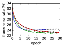
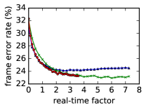
Figure 1: Development set frame error rates vs. number of epochs (left) and vs. training real-time factor (time spent training / duration of training set, right).

Table 1: Real-time factors for decoding per sample and hours for training the system.

	decoding (RT)						training (hours)
	1st pass	2nd pass	3rd pass	total decoding	feeding forward	total overall	1st pass	2nd pass	3rd pass	total training	feeding forward	total overall
baseline	0.33	0.01		0.34	0.33	0.67	49.5	0.6		50.1	59.4	109.5
proposed	0.11	0.02	0.01	0.14	0.17	0.31	1.0	1.2	0.6	2.8	29.7	32.5

6.2 Segmental cascade experiments

Our baseline system is a discriminative segmental model $R$ based on [10], which is a first-pass segmental model using the following segment features: log posterior averages, log posterior samples, log posteriors at the boundaries, segment length indicators, and bias. See [10] for more complete descriptions of the features. All features are lexicalized with label unigrams. The baseline system is trained by optimizing hinge loss with AdaGrad using mini-batch size 1, step size 0.1, and early stopping for 50 epochs.

Recall that the proposed two-feature first-pass system is a segmental model $A_{1}$ with just the label posterior and bias features. We use hinge loss optimized with AdaGrad with mini-batch size 1 and step size 1. None of the features are lexicalized. Since we only have two features, learning converges very quickly, in only three epochs. We take the model from the third epoch to produce lattices for subsequent passes in the cascade.

Given $A_{1}$, we compare lattices generated by $A_{1}$ with different pruning methods. We consider $\alpha_{\text{edge}}\in\{0.8,0.85,0.9\}$ for edge pruning, $\alpha_{\text{vertex}}\in\{0.925,0.95,0.975\}$ for vertex pruning, and $\alpha_{\text{beam}}\in\{0.93,0.94,0.95,0.96\}$ for beam pruning. The results are shown in Figure 2. We observe that edge pruning generally gives the best density-oracle error rate tradeoff. Beam search is inferior in terms of speed and lattice quality.

We also measure real-time factors for different pruning methods, shown in Figure 2. We can see that all pruning methods can obtain oracle error rates less than 2% within 0.1 $\times$ real-time. No single pruning method is significantly faster than the others. Intuitively, while max-marginal pruning requires more computation per edge, it makes more informed decisions. The bottom line is that max-marginal pruning produces less-dense lattices with the same performance in the same amount of time.

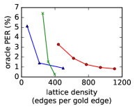
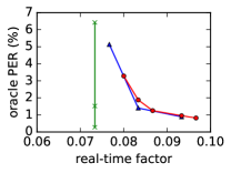
Figure 2: Left: Densities versus oracle error rates of lattices generated by different pruning methods. Right: Time spent on generating the lattices with different pruning methods.

Based on the above experiments, we use lattices produced by edge pruning with $\alpha_{\text{edge}}=0.85$ for the remaining experiments, because the lattices are sparse and have only 1.4% oracle error rate. We train a second-pass model $A_{2}$ with the same features as the baseline system $R$ except that we add a “lattice score” feature corresponding to the segment score given by the two-feature system $A_{1}$. Hinge loss is optimized with AdaGrad with mini-batch size 1, step size 0.1, and early stopping for 20 epochs.

The learning curve comparing $R$ and $A_{1}$ followed by $A_{2}$ is shown in Figure 3. We observe that the learning time per epoch of the two-feature system $A_{1}$ is only one-third of the baseline system $R$. We also observe that training of $A_{2}$ converges faster than training $R$, despite the fact that they use almost identical feature functions. The baseline system achieves the best result at epoch 49. In contrast, the two-pass system is done before the baseline even finishes the third epoch.

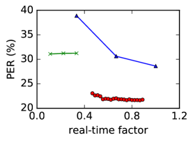
Figure 3: Learning curve of the proposed two-pass system compared with the baseline system. The time gap between the first pass and the second pass is the time spent on pruning.

Following [10], given the first-pass baseline, we apply max-marginal edge pruning to produce lattices for the second-pass baseline with $\alpha_{\text{edge}}=0.8$. The second-pass baseline features are the lattice score from the first-pass baseline, a bigram language model score, first-order length indicators, and a bias. Hinge loss is optimized with AdaGrad with mini batch size 1, step size 0.01, and early stopping for 20 epochs. For the proposed system, we produce lattices with edge pruning and $\alpha_{\text{edge}}=0.3$ for the third-pass system. We use the same set of features and hyper-parameters as the second-pass baseline for the third pass.

Phone error rates of all passes are shown in Table 2. First, if we compare the one-pass baseline with the proposed two-pass system, our system is on par with the baseline. Second, we observe a healthy improvement by just adding the bigram language model score to the second-pass baseline. The improvement for our third-pass system is small but brings our final performance to within 0.4 of the baseline second pass.

Table 2: Phone error rates (%) of proposed and baseline systems.

		1st pass	2nd pass	3rd pass
baseline	dev	21.9	21.0
	test	24.0	23.0
proposed	dev	33.6	21.5	21.3
	test		23.7	23.4

Next we report on the speedups in training and decoding obtained with our proposed approach. Table 1 shows the real-time factors for decoding with the baseline and proposed systems. In terms of decoding time alone, we achieve a 2.4 time speedup compared to the baseline. If the time of feeding forward LSTMs is included, then our proposed system is two times faster than the baseline.

Table 1 shows the times needed to train a system to get to the performance in Table 2. The speedup mostly comes from the fast convergence of the first pass. In terms of training the segmental models alone, we achieve an 18.0-fold speedup. If the time to train the LSTMs is included, then we obtain a 3.4-fold speedup compared to the baseline.

To summarize some of the above results: With a combination of the first-pass two-feature system and edge pruning, we prune 95% of the segments in the first-pass hypothesis space, leading to significant speedup in both decoding and training. The feed-forward time for our LSTMs is halved through frame subsampling. In the end, with a single four-core CPU, we achieve 0.31 times real-time decoding including feeding forward, which is 2.2 times faster than the baseline, and 32.5 hours in total to obtain our final model including LSTM training, which is 3.4 times faster than the baseline. Excluding the LSTMs, the segmental model decoding alone is 2.4 times faster than the baseline, and training the segmental models alone is 18 times faster than the baseline.

7 Conclusion

We have studied efficiency improvements to segmental speech recognition structured as a discriminative segmental cascade. Segmental cascades allow us to push features around between different passes to optimize speed and performance. We have taken advantage of this and proposed an extremely simple first-pass segmental model with just two features, a label posterior and a bias, which is intuitively like a segmental analogue of a typical hybrid model. We have also compared pruning approaches and find that max-marginal edge pruning is the most effective in terms of time, lattice density, and oracle error rates. With the combination of these measures and frame subsampling for our input LSTMs, we obtain large gains in decoding and training speeds. With decoding and training now being much faster, future work will explore even richer feature functions and larger-scale tasks such as word recognition.

8 Acknowledgements

This research was supported by a Google faculty research award and NSF grant IIS-1433485. The opinions expressed in this work are those of the authors and do not necessarily reflect the views of the funding agency. The GPUs used for this research were donated by NVIDIA.

References

- [1] J. Glass, “A probabilistic framework for segment-based speech recognition,” Computer Speech & Language, vol. 17, no. 2, pp. 137–152, 2003.
- [2] G. Zweig and P. Nguyen, “A segmental CRF approach to large vocabulary continuous speech recognition,” in IEEE Workshop on Automatic Speech Recognition & Understanding, 2009, pp. 152–157.
- [3] S.-X. Zhang, A. Ragni, and M. J. F. Gales, “Structured log linear models for noise robust speech recognition,” Signal Processing Letters, IEEE, vol. 17, no. 11, pp. 945–948, 2010.
- [4] G. Zweig, P. Nguyen, D. V. Compernolle, K. Demuynck, L. Atlas, P. Clark, G. Sell, M. Wang, F. Sha, H. Hermansky, D. Karakos, A. Jansen, S. Thomas, G. Sivaram, S. Bowman, and J. Kao, “Speech recognition with segmental conditional random fields: A summary of the JHU CLSP 2010 summer workshop,” in IEEE International Conference on Acoustics, Speech and Signal Processing, 2011, pp. 5044–5047.
- [5] M. D. Wachter, M. Matton, K. Demuynck, P. Wambacq, R. Cools, and D. V. Compernolle, “Template-based continuous speech recognition,” Audio, Speech, and Language Processing, IEEE Transactions on, vol. 15, no. 4, pp. 1377–1390, 2007.
- [6] O. Abdel-Hamid, L. Deng, D. Yu, and H. Jiang, “Deep segmental neural networks for speech recognition.” in Proceedings of the Annual Conference of International Speech Communication Association, 2013, pp. 1849–1853.
- [7] Y. He, “Segmental models with an exploration of acoustic and lexical grouping in automatic speech recognition,” Ph.D. dissertation, Ohio State University, 2015.
- [8] L. Lu, L. Kong, C. Dyer, N. A. Smith, and S. Renals, “Segmental recurrent neural networks for end-to-end speech recognition,” arXiv preprint arXiv:1603.00223, 2016.
- [9] Y. He and E. Fosler-Lussier, “Efficient segmental conditional random fields for phone recognition,” in Proceedings of the Annual Conference of the International Speech Communication Association, 2012, pp. 1898–1901.
- [10] H. Tang, W. Wang, K. Gimpel, and K. Livescu, “Discriminative segmental cascades for feature-rich phone recognition,” in IEEE Workshop on Automatic Speech Recognition & Understanding, 2015.
- [11] S. Hochreiter and J. Schmidhuber, “Long short-term memory,” Neural computation, vol. 9, no. 8, pp. 1735–1780, 1997.
- [12] H. Tang, K. Gimpel, and K. Livescu, “A comparison of training approaches for discriminative segmental models,” in Proceedings of the Annual Conference of International Speech Communication Association, 2014.
- [13] V. Steinbiss, B.-H. Tran, and H. Ney, “Improvements in beam search,” in ICSLP, vol. 94, no. 4, 1994, pp. 2143–2146.
- [14] X. L. Aubert, “An overview of decoding techniques for large vocabulary continuous speech recognition,” Computer Speech & Language, vol. 16, no. 1, pp. 89–114, 2002.
- [15] A. Sixtus and S. Ortmanns, “High quality word graphs using forward-backward pruning,” in IEEE International Conference on Acoustics, Speech and Signal Processing, 1999, pp. 593–596.
- [16] D. Weiss, B. Sapp, and B. Taskar, “Structured prediction cascades,” 2012, arXiv:1208.3279 [stat.ML].
- [17] V. Vanhoucke, M. Devin, and G. Heigold, “Multiframe deep neural networks for acoustic modeling,” in IEEE International Conference on Acoustics, Speech and Signal Processing (ICASSP). IEEE, 2013, pp. 7582–7585.
- [18] Y. Miao, J. Li, Y. Wang, S. Zhang, and Y. Gong, “Simplifying long short-term memory acoustic models for fast training and decoding,” in IEEE International Conference on Acoustics, Speech and Signal Processing, 2015.
- [19] J. Duchi, E. Hazan, and Y. Singer, “Adaptive subgradient methods for online learning and stochastic optimization,” The Journal of Machine Learning Research, vol. 12, pp. 2121–2159, 2011.
- [20] W. Zaremba, I. Sutskever, and O. Vinyals, “Recurrent neural network regularization,” arXiv preprint arXiv:1409.2329, 2014.