Vortex knots in tangled quantum eigenfunctions

Abstract

Tangles of string typically become knotted, from macroscopic twine down to long-chain macromolecules such as DNA. Here we demonstrate that knotting also occurs in quantum wavefunctions, where the tangled filaments are vortices (nodal lines/phase singularities). The probability that a vortex loop is knotted is found to increase with its length, and a wide gamut of knots from standard tabulations occur. The results follow from computer simulations of random superpositions of degenerate eigenstates of three simple quantum systems: a cube with periodic boundaries, the isotropic 3-dimensional harmonic oscillator and the 3-sphere. In the latter two cases, vortex knots occur frequently, even in random eigenfunctions at relatively low energy, and are constrained by the spatial symmetries of the modes. The results suggest that knotted vortex structures are generic in complex 3-dimensional wave systems, establishing a topological commonality between wave chaos, polymers and turbulent Bose-Einstein condensates.

Complexity in physical systems is often revealed in the subtle structures within spatial disorder. In particular, the complex modes of typical 3-dimensional domains are not usually regular, and at high energies behave according to the principles of quantum ergodicityT ; H . The differences between chaotic and regular wave dynamics can be seen clearly in the Chladni patterns of a vibrating two-dimensional plateH , in which the zeros (nodes) of the vibration accumulate small sand particles to appear as random curved lines when the plate is irregular. The spatial distribution of these nodal lines is statistically isotropic at high energiesH , and this irregularity is typical for chaotic systems, whose ergodic dynamics are determined only by the energy and there are no other constants of motion.

Understanding the spatial structure of these wavefunctions can be challenging. Following the hydrodynamic interpretation of single-particle quantum mechanicsmadelung27 , the zeros of three-dimensional complex-valued scalar fields are, in general, lines, which are vortex filaments around which the phase, local velocity and probability current (in a quantum wavefunction) circulated ; riess70 ; E . This is analogous to the vortices of a classical fluid, although the phase change around the vortex line is quantised in units of 2$\pi$, and is singular at the vortex core where the amplitude is zero. A similar vortex topology occurs in condensates of many quantum particlesM . The pattern of their vortex lines provides a structural skeleton to wavefunctionsd ; E ; dennis09 . In modes above the lowest energies, the vortex pattern is far from regular and they are densely intertwined. A natural three-dimensional measure of the most extreme spatial irregularity is when the vortex filaments are knotted, and here we study the occurrence of knotted nodal vortex lines in three model systems of wave chaos, as a natural extension of the Chladni problem to three dimensions.

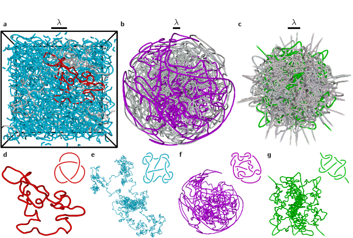
FIG. 1: Tangled and knotted vortex filaments in random high-energy eigenfunctions of energy $E_{N}$. Vortex lines are shown in a a periodic cubic cell, with principal quantum number $N=9$ ($E_{N}\propto 3N^{2}$); b the 3-sphere (plotted in a distorted projection in which all points on the bounding sphere are equivalent) with $N=17$ ($E_{N}\propto N(N+2)$), and c the three-dimensional harmonic oscillator with $N=21$ ($E_{N}\propto N+3/2$). The total vortex length is similar in each eigenfunction, a reference wavelength at the origin, proportional to $E_{N}^{-1/2}$ is given in each of a, b, c. Each vortex loop in the eigenfunction is coloured grey except for one or two knotted examples in each system, illustrated further in d-g; each of these coloured knots is plotted alongside a simpler projection of the same knot: d the trefoil knot (tabulated as $3_{1}$ G ; X ) from a, with length $L=50~{}\lambda$ and determinant $|\Delta(-1)|=3$; e a composite knot consisting of the two trefoils joined with the 6-crossing knot $6_{2}$ (i.e. $3_{1}^{2}\#6_{2}$), which passes through the periodic boundary of a many times with $L=$1700$~{}\lambda$ and $|\Delta(-1)|=99$; f the more complicated 14-crossing prime knot from b, labelled $K14n5049$ in the extended notation of standard tabulations beyond $11$ crossingsX , with $L=$1500$~{}\lambda$ and $|\Delta(-1)|=313$; g the open 8-crossing prime knot $8_{12}$ from c, having $L=$1000$~{}\lambda$ where $\lambda$ is defined with respect to momentum at the origin and only vortex length in the classically allowed region is considered, and with $|\Delta(-1)|=29$.

Despite numerous investigations of the physics of diverse random filamentary tangles, including quantum turbulencebarenghi07 , loop soupsZ , cosmic strings in the early universevilenkin , and optical vortices in 3-dimensional laser speckle patternsR , the presence of knotted structures in generic random fields has not been previously emphasized or systematically studied. Vortices and defects which are knotted have been successfully embedded in a controlled way in various 3-dimensional fields, such as vortex knots in waterN , knotted defects in liquid crystalsO ; P and knotted optical vortices in laser beamsQ , and theoretically as vortex lines in complex scalar fields, including superfluid flowskleckner16 , and superpositions of energy eigenstates of the quantum hydrogen atombb and other wave fieldsbd01 , but rigorous mathematical techniques to resolve the statistical topology of random fields are limitedS . With modern high-performance computers, the structure can be explored using large-scale simulations.

In the following, we investigate the knottedness of the nodal vortex structures in typical chaotic eigenfunctions of comparable size (i.e. energy and total nodal line length) for three model systems. The chaotic eigenfunctions are represented as superpositions of degenerate energy eigenfunctions weighted by complex, Gaussian random amplitudes; such superpositions are established as good models of wave chaos in the semiclassical limit of high energy F ; H ; T , since the wave pattern is determined only by their energy (unlike a plane wave which has a well-defined momentum). Our three systems are the cubic cell with periodic boundary conditions, whose degenerate eigenfunctions are plane waves; the abstract 3-dimensional sphere (3-sphere), whose degenerate eigenfunctions are hyperspherical harmonics and which has finite volume but no boundary; and the isotropic, 3-dimensional harmonic oscillator (3DHO), whose nodal structure is largely contained within the classically allowed region where energy exceeds the potential, such as could describe an isotropic harmonically-trapped Bose-Einstein condensateL . Further information and illustrations of these eigenfunction systems appear in Supplementary Note 1 and Supplementary Figures 1-4.

We find that vortex knots occur with high probability at sufficiently high energy in all of these random wave superpositions. Even in low energy cavity modes, possibly accessible to experiments, the results suggest knotted vortices will occur with some reasonable probability. The statistical details of random vortex knotting (with respect to the types of knot that occur, the length of knotted vortex curves, and the eigenfunction energy) depends strongly on the wave system, and we perform an analysis and comparison of these properties.

Results

Knots in high energy random eigenfunctions

Figure 1 shows the nodal/vortex structure of a typical chaotic eigenfunction in each model system: in 1a, a cube with periodic boundaries; in 1b, the 3-sphere; and in 1c, the 3DHO. In all three cases the random modes are labelled by energy $E_{N}$ with principal quantum number $N$ (further details of how the model systems are generated and how the vortices are located is given in Supplementary Notes 1 and 2). In each of Figures 1d-g, a single vortex line from these eigenfunctions is shown alongside a simpler projection of the same knot. Each vortex line resembles a random walk U ; R .

Our analysis of these knots uses the standard conventions of mathematical knot theoryG , in which knots in closed curves can be factorised into prime knots which are tabulated according to their minimum number of crossings (examples are shown in Supplementary Figure 5). Both prime knots (e.g. as Figure 1d,f-g), and composites of prime knots (e.g. as Figure 1e), are identified in the curve data by a combination of several schemes. After simplifying the longest curves by a geometric relaxation methodU , several topological invariants are computed for each curve, which distinguish knots of different types. These are: the absolute value of the Alexander polynomialk $|\Delta(t)|$, evaluated for $t$ at certain roots of unity; the hyperbolic volumeV ; and the second and third order Vassiliev invariantsJ ; W . Although other knot invariants can have more discriminatory power than these separately G ; X , they tend to be significantly more demanding in computer time: in practice the combination of this particular set of invariants discriminates almost all tabulated knotsG ; X (up to at least 14 crossings; the methods are described further in Supplementary Note 3). Each of these invariants encodes different topological and geometric information about each knotG . When comparing the knottedness of different vortex loops, we follow previous studiesk ; J in using the (positive integer-valued) knot determinant $|\Delta(-1)|$ as the primary quantitative measure of their knotting complexity.

We have identified approximately $50000$ knots from around $10^{9}$ curves (of different lengths), computed from about $10^{6}$ random eigenfunctions (at different energies). Some of these knotted curves are relatively short (such as that in Figure 1d), although the majority of vortex knots are much longer, such as in Figure 1e, whose full spatial extent spreads over several periodic cells. At large lengthscales, each curve approximates a Brownian random walkU ; R ; for closed curves, the radius of gyration scales with the square root of the total length. Most of the vortex knots occur in closed loops; in the 3DHO, however, most vortex lines stretch to spatial infinity as almost-straight lines in the classically forbidden region. Most of the knots in the 3DHO are in these open curves, such as that represented in Figure 1g. In the periodic cube, many of the longer lines wrap around the cell a nonzero number of times (i.e. they have nontrivial homology, so in a tiling of the 3D cells they would be infinitely long and periodicR ). Since knots in such a periodic space have not been adequately classified mathematicallyG , we only consider knots in closed loops with trivial homology in this system.

Links, which are configurations of two or more vortex curves that are topologically entangled with one another, also occur frequently. In fact we find links to be more common than knots, consistent with previous investigations of random optical fields at smaller lengthscales in which links are found to be common but knots were not detectedae . The restriction to knotting in the present study was chosen as it allows comparison with extensive studies of the knotting probability of random curves (as random walks)k , whereas the study of random linking is not so well developed. Furthermore, linking of open curves (in the 3DHO) is not well-defined. For these reasons, our analysis is limited to the statistics of vortex knotting.

Probabilities and complexities of knottedness

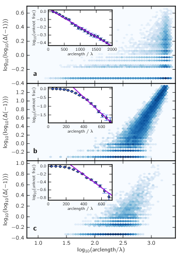
FIG. 2: Dependence of vortex knot complexity on curve length. The plots show histograms of $\log_{10}(\log_{10}|\Delta(-1)|)$ against $\log_{10}(L)$ for the thee systems at the same energies of the examples in Figure 1: a periodic cube, $N=9$; b 3-sphere, $N=17$; c three-dimensional harmonic oscillator, $N=21$. In each system, the logarithm of the probability that a given vortex curve is unknotted as a function of its length $L$ is plotted in the insets, with error bars representing the standard error on the mean probability over many different random eigenfunctions. For larger values of $L$, this unknotting probability logarithm is fitted to $-L/L_{0}+\mathrm{const}$, with scaling factors $L_{0}$ of approximately: a $$1800$~{}\lambda$; b $100~{}\lambda$; c $250~{}\lambda$. In the main plots, the strong horizontal lines of constant, low-value $|\Delta(-1)|$ correspond to specific knots, such as the trefoil (for which $\log_{10}(\log_{10}|\Delta(-1)|)=-0.32$) and the composite double trefoil $3_{1}\#3_{1}$ (for which $\log_{10}(\log_{10}|\Delta(-1)|)=-0.02$).

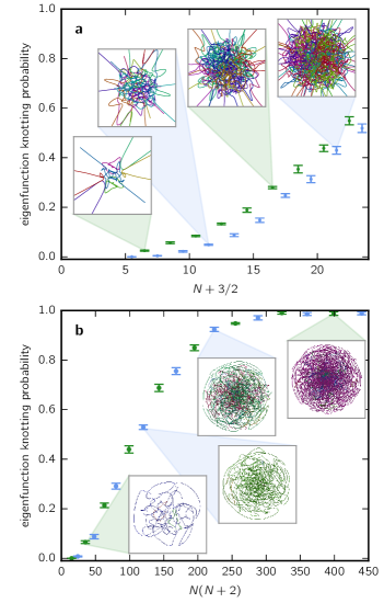
FIG. 3: Probabilities that, as functions of energy, a given random eigenfunction in the system contains knotted vortices. a three-dimensional harmonic oscillator; b 3-sphere. Blue (green) points denote those where the principal quantum number $N$ is even (odd), for reasons described in the main text, and errors represent the standard error on the mean fraction of knotted eigenfunctions, averaged over many different random samples. Insets depict the vortices in a typical eigenfunction at different energies, with each vortex curve is represented in a different colour.

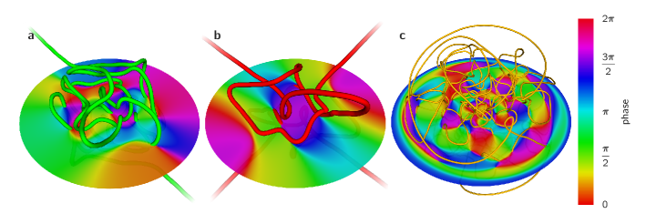
FIG. 4: Examples of low-energy eigenfunctions with knotted vortices in symmetric strongly amphicheirally symmetric conformations. a three-dimensional harmonic oscillator (3DHO), $N=5$, with a single open figure-8 vortex knot (tabulated as $4_{1}$) in a strongly negatively amphicheiral conformation (this is the simplest prime knot with this symmetry); b 3DHO, $N=4$, with a pair of mirrored trefoil vortex knots $3_{1}\#3_{1}$ (knotting at this low energy is found to be extremely rare); c 3-sphere, $N=7$, with the knot $10_{99}$ (the simplest prime knot with strongly positive amphicheiral symmetryAA ), but omitting the two other small vortex loops occurring in this eigenfunction. In each case, the phase in a plane through the centre of the complex random wavefunction is represented, coloured by hue. Supplementary Movies 1-3 show these wavefunctions from varying viewpoints.

As one might expect, the random eigenfunction statistics show that longer knotted vortex curves display a greater complexity of knot types, as measured by the knot determinant $|\Delta(-1)|$. This is represented in Figure 2 for each of the three systems at fixed energy. These histograms indicate that the distribution of $\log|\Delta(-1)|$ with respect to vortex length $L$ apparently scales according to a power law. Longer curves are also more likely to be knotted; the probability of a given vortex loop being unknotted decreases exponentially according to $L$ (Figure 2 insets), as previously studied for random walks modelling polymersI ; J ; k . The value of the unknotting exponents is different for each of the three systems, given in the caption.

Each of the model systems studied has a finite spatial extent: the side length of the cube, and the diameters of the 3-sphere and classically-allowed region of the 3DHO. In the latter two cases, this finite size imposes a long-length cutoff $S$ to the Brownian scaling of long vortex lines. In the 3-sphere and 3DHO, loops whose radius of gyration exceeds $S$ are confined, and the Brownian and confined regimes have different knotting probability exponents. Both knotting probability and complexity increase distinctly with length in the confined regime, where long curves are restricted to volumes much smaller than the corresponding Brownian radius of gyration would allow.

In contrast, the cube’s periodic boundary conditions allow the vortex lines to have extent greater than the cube side length, although the Brownian scaling of loop sizes gives way at some $S$ to the lines with nontrivial homology, which do not contribute to the knot count. Figure 2b,c shows that the minimal complexity of knots in the confined regime also scales with $L$; long vortices are always knotted in these systems, and the knot is usually very complex. By contrast, under periodic boundary conditions (Figure 2a) even the longest vortex loops can be topologically trivial. In all of these cases, the scaling depends weakly on the energy of the eigenfunction, at least in the ranges of energy considered in the simulations.

Low energy knots and the impact of eigenfunction symmetry

The total vortex length in random eigenfunctions is proportional to their energy $E_{N}$ (see Supplementary Note 1). It is therefore natural to expect knotted vortex lines to occur more frequently in higher-energy eigenfunctions. This probability of knotting with energy is shown in Figure 3 for eigenfunctions of the 3-sphere and 3DHO. In the 3-sphere, where all vortex loops must be closed, this probability reaches 99% when $N\approx 16$, which is surprisingly small to guarantee such a degree of topological complexity (as illustrated in the insets).

The energies simulated in the 3DHO are insufficient to guarantee that a random eigenfunction will contain a knotted vortex (Figure 3a), as the distribution of vortex lengths in the classically allowed region prefers a greater number of shorter curves. The knotting probability of a 3DHO eigenfunction also strongly depends on whether the principal quantum number $N$ is odd or even, since 3DHO energy eigenstates, and hence the zeroes (i.e. the vortex tangle), must be parity-symmetric with respect to spatial inversion through the origin; in fact, the nodal system of vortex curves is required to be strongly negatively amphicheiralAA (i.e. the tangents at parity-opposite vortex points must be parallel). Furthermore, when $N$ is odd, exactly one open vortex line must pass through the origin, such as the low-energy example in Figure 4a. Since strongly negatively amphicheiral knots must be open (see Supplementary Note 4 and Supplementary Figure 6), this line can take such a configuration and is commonly knotted, contributing to a larger knotting probability when $N$ is odd (other knots can occur when $N$ is odd or even, but only in antipodal pairs, as in Figure 4b). This symmetry constraint applies to all energies considered in the simulations.

Eigenfunctions of the 3-sphere must also be symmetric under inversion between antipodal points, but here the curve system must be strongly positively amphicheiral (opposite vortex points have antiparallel tangents). The simplest prime knot with this symmetry is in fact the 10-crossing knot $10_{99}$AA , and an example of a knotted vortex of this type is shown in Figure 4c.

Discussion

Based on computer experiments, we have shown that knotted vortex lines are common in random quantum wavefunctions, even at comparatively low energies. These results complement previous rigorous mathematical studies where small knots (of any type) have been proven to occur with nonzero probability in random eigenfunctions of the 3DHOac and hydrogen atomperaltasalashydrogen at high energies. These knots would be quite different from those studied in the present work, as they occupy limited volumes and, in the 3DHO, occur with exponentially small probabilities. As such, those knots may be thought of as highly structured superoscillatory phenomenaberry94 , known to be very rare. On the other hand, the knotted vortices emphasised here can extend throughout the entire wavefunction, and are rather common except at the lowest energies; in fact, the very smallest knots we find in the 3DHO are an order of magnitude larger than the bounds on the size of superoscillatory examples. Preliminary numerical studies of vortex knots in random eigenfunctions of hydrogen indicate similar behaviour to the 3DHO described here, where eigenfunctions containing knotted vortices are typical beyond a certain energy (and comparable mode count), although unlike the 3DHO and 3-sphere, the nodal sets are not constrained by an amphicheiral symmetry.

Although our computer experiments have been limited to modes of fixed energy, we do not anticipate major differences in systems of random waves with different power spectra, such as a turbulent Bose-Einstein condensateL with characteristic power law spectrum, especially when sizes of system are similar to or greater than those considered here.

Knotting of vortices in chaotic complex 3D eigenfunctions is a complex counterpart to Chladni’s original observation of the structure of cavity modes, and we anticipate that generic 3D complex cavity modesH ; T will contain knotted vortices. Our results lead us to expect that almost every random quantum eigenfunction at sufficiently high energy contains at least one knotted vortex line and, at least in the systems considered here, this is common even at the relatively low energies currently accessible to numerical experiment. Knotted nodal lines with characteristic complexity scalings may therefore be a complex, 3-dimensional counterpart to the nodal statistics proposed to signify quantum chaosad for real-valued chaotic eigenfunctions in two dimensions. Based on the mode countsH of the energies in Figure 3, we expect knotted vortices to occur with 50% probability from somewhere between the 500th (3-sphere) to $3000$th (3DHO) mode of a chaotic cavity.

Methods

Sampling random eigenfunctions. We generate random eigenfunctions of model systems via standard random superpositions of their degenerate eigenfunctions. Further details and comparisons of these systems, especially their eigenfunctions, are included in Supplementary Note 2.

Tracking vortices (nodal lines). Within each random eigenfunction, phase vortices are numerically tracked by sampling the wavefunction on a cubic lattice (initial voxel size approximately $0.1\lambda$) and checking around each numerical grid plaquette for the circulation of phase indicating the passage of a vortex line through the face of the grid cell. The phase is only guaranteed to circulate in this way when the amplitude is zero but the complex scalar gradient is non-zero (i.e. the vortices occur as transverse intersections of real and imaginary nodal surfaces), but this is generically the case in random eigenfunctions; the algorithm would otherwise fail to converge on the vortex line but, as anticipated, we have never observed this to happen. This core procedure does not always fully capture the geometry of the vortex curve (especially where two vortex lines approach closely), and so the above procedure is augmented with a recursive resampling of the numerical grid, at successively higher resolutions, in any location where the vortex line tracking is ambiguous; we call this the RRCG algorithm (see Supplementary Note 2). Since vortex lines must be continuous, the result of the algorithm is a piecewise-linear representation of each vortex in the entire large scale tangle. The vortex topology is retained, and geometry well recovered, even with a relatively poor initial sampling resolution. The algorithm generalises to each of periodic boundary conditions, the 3-sphere and the 3DHO via an appropriate choice of lattice boundary conditions, and in the case of the 3-sphere by sampling on multiple Cartesian lattices and joining appropriate boundaries to reproduce the geometry of the sphere.

Detecting and classifying knots and links. The topology of vortices is investigated using the standard knot invariants described in the main text, whose values depend only on the topology of a single curve and from which the knot type can be inferred. It is computationally expensive to use some invariants known to be more powerful (e.g. the Jones or HOMFLY-PT polynomials), or to identify the exact knot type of every curve. When necessary (Figure 1, Figure 4) we are able to do so unambiguously using the Alexander polynomial (evaluated at certain roots of unity), hyperbolic volume, and Vassiliev invariants or degree 2 and 3. We further use the knot determinant to measure the topological complexity of vortex curves even without identifying their specific knot types.

Data availability

All relevant data are available from the corresponding author upon request.

Author contributions

A J Taylor created the numerical routines for simulating eigenfunction modes and performing topological analysis. Other contributions were shared equally.

Supplementary Note 1:
Random wave formulation and nodal statistics

The wavefunctions whose nodal structures are considered in the main text are random superpositions of degenerate energy eigenstates in a given system, considered over 3-dimensional position $\vec{r}=(x,y,z)$,

$$\psi_{j}^{N}(\vec{r})=\sum_{j}a_{j}\Psi^{N}_{j}(\vec{r})$$ (1)

where the sum is over a finite set of indices labelled by $j$, the $a_{j}$ are Gaussian random complex variables, and the $\Psi^{N}_{j}$ satisfy the time-independent Schrödinger equation $\hat{H}\Psi^{N}_{j}=E\Psi^{N}_{j}$ for some 3-dimensional Hamiltonian operator $\hat{H}$. Thus $\hat{H}\psi_{N}=E\psi_{N}$, and $N$ denotes an integer quantum number.

In the usual random wave model (RWM) which is taken to model wave chaos (for instance, quantum chaotic eigenfunctions in the semiclassical limit) F ; L , the Hamiltonian is $\hat{H}=-\tfrac{\hbar^{2}}{2M}\nabla^{2}$ for a single particle of mass $M$ at a high energy, so the sum over $j$ is effectively infinite. The ensemble of random functions is statistically isotropic, homogeneous and ergodic, and the (non-normalizable) basis states $\Psi_{j}$ can be taken to be plane waves with the same spatial frequency $\Psi_{j}(\vec{r})=\exp(i\vec{k}_{j}\cdot\vec{r})$, where $E=\tfrac{\hbar^{2}}{2M}|\vec{k}_{j}|^{2}$.

Unlike the RWM, our numerical realisations are systems involving superpositions over a finite number of degenerate energy eigenfunctions (indexed by principal quantum number $N$), whose spatial complexity only occupies a finite spatial volume yet whose spatial configuration (including the vortex lines) is statistically similar to the RWM. These systems are the periodic cubic cell, the 3-sphere and the isotropic three-dimensional harmonic oscillator (3DHO). The statistical behaviour of the eigenfunctions of each of these systems approaches that of the isotropic RWM in the limit of high energy. We compare these systems at a range of different energies, from those where knotted vortices first appear to the highest energies practically accessible using the RRCG algorithm introduced in Section Supplementary Note 2: Numerical techniques. Sample functions of the two-dimensional analogues of these complex random fields are shown in Supplementary Figure 1, where the vortices occur as points (nodes of modulus, phase singularities).

The periodic 3-cell (flat 3-torus) of side length $L$ has the most direct connection to the treatment of the infinite bulk RWM. The Hamiltonian is again $-\tfrac{\hbar^{2}}{2M}\nabla^{2}$ and the eigenfunctions are plane waves with Cartesian components proportional to integers, $\vec{k}_{j}=\tfrac{2\pi}{L}(\ell,m,n)$. The corresponding energy is $\tfrac{2\pi^{2}\hbar^{2}}{ML^{2}}(\ell^{2}+m^{2}+n^{2})$, and the degeneracies follow naturally from different triplets of integers having the same sum of squares, with $j$ acting as an index over such triplets.

An extra consideration determines which eigenfunctions of the periodic cell are chosen for our study of vortex tangling. For a typical eigenfunction, the complex field $\psi_{N}$ is periodic with a cubic fundamental cell. However, it is not difficult to show that for any such $\psi$, if $\psi(\vec{r})=0$, then $\psi\left(\vec{r}+\tfrac{L}{2}(1,1,1)\right)=0$ and hence the periodicity of a typical eigenfunction’s nodal structure is body-centred cubic. The primitive cell of such a lattice, and therefore of the nodal line tangle, is a truncated octahedron. For simplicity in numerically tracking vortices through the periodic boundaries, we prefer to describe a periodic nodal structure whose primitive cell is a cube. These symmetries of nodal lines in a larger field with cubic symmetry are illustrated in Supplementary Figure 2.

Certain energies give rise to extra symmetries which guarantee this property. When energies are chosen to be $E=\tfrac{2\pi^{2}\hbar^{2}}{ML^{2}}3N^{2}$ for integer $N$, that is, $\ell^{2}+m^{2}+n^{2}=3N^{2}$, then $\ell,m,n$ must be all odd or all even, depending on whether $N$ is odd or even. The nodal structure of a superposition of these plane waves has a primitive cell which is cubic with side length $L/2$, which is an octant of the original cubic cell of the complex wavefunction. It is these smaller cells which are considered in the main text. Energies $E_{N}\propto 3N^{2}$ are guaranteed to have at least an eightfold degeneracy with $(\ell,m,n)=(\pm N,\pm N,\pm N)$, and in practice (for sufficiently high $N$) the degeneracy is much higher. In the examples in the main text, $N$ is chosen to be $9$, so triplets of integers whose sum of squares equals 243 are 3,3,15; 5,7,13; 1,11,11 as well as 9,9,9. All together, the total number of plane waves at this energy (counting permutations and all possible signs of components) is 104. The nodal statistics for random eigenfunctions at this energy closely recover local geometrical statistics expected of the isotropic model U .

In the 3-sphere, coordinates are specified in terms of three angles, $\chi,\theta,\phi,$ with $0\leq\chi,\theta\leq\pi,0\leq\phi<2\pi$. The energy eigenfunctions are those of the (normalised) Laplace-Beltrami operator on the 3-sphere, which are the hyperspherical harmonics hochstadt71 ,

$$\mathcal{Y}_{N\ell m}(\chi,\theta,\phi)=\sqrt{\frac{2^{2\ell+1}(N-\ell)!(1+N)}{\pi(1+\ell+N)!}}\,\ell!\,\sin^{\ell}(\chi)\,C_{N-\ell}^{(\ell+1)}(\cos\chi)\,Y_{\ell}^{m}(\theta,\phi)~{},$$ (2)

where $Y_{\ell}^{m}$ are the usual spherical harmonics of the 2-sphere, $C_{N-\ell}^{(\ell+1)}$ are Gegenbauer polynomials, and for integers $N,\ell,m$, $0\leq N$, $0\leq\ell\leq N$ and $-\ell\leq m\leq\ell$. The corresponding eigenvalues are labelled by the principal quantum number $N$, with $E_{N}=N(N+2)$ (in appropriate units) which are therefore $(N+1)^{2}$-fold degenerate with the label $j$ corresponding to different values of $\ell$ and $m$. In the main text, nodal structures are calculated in these systems for $N$ up to 21. In the stereographic projection of the 3-sphere into spherical polar coordinates, $\theta$ and $\phi$ are the usual spherical angles, and the radial coordinate is $\tan(\chi/2)$.

Random waves in the 3DHO are randomly weighted degenerate eigenfunctions of the Laplacian with an isotropic harmonic potential with angular frequency $\omega$,

$$\hat{H}\psi_{N}=-\tfrac{\hbar^{2}}{2m}\nabla^{2}\psi_{N}(\vec{r})+\tfrac{m\omega^{2}}{2}\vec{r}^{2}\psi_{N}(\vec{r})=E_{N}\psi_{N}(\vec{r})~{},$$

where $E_{N}=\hbar\omega(N+\tfrac{3}{2})$ for integer $N\geq 0.$ Following the standard theory of the three dimension isotropic harmonic oscillator, the energy eigenfunctions are $\tfrac{1}{2}(N+1)(N+2)$-fold degenerate rae07 . Multiple different bases of energy eigenfunctions can be chosen, but the simplest option for numerical computation utilises Hermite polynomials $H_{n}$ arising from separation of variables in Cartesian coordinates,

$$\Psi^{N}_{j}(\vec{r})=\frac{1}{\sqrt{2^{N}\ell!m!n!}}\left(\frac{M\omega}{\pi\hbar}\right)^{3/2}H_{\ell}\left(\sqrt{\tfrac{M\omega}{\hbar}}x\right)H_{m}\left(\sqrt{\tfrac{M\omega}{\hbar}}y\right)H_{n}\left(\sqrt{\tfrac{M\omega}{\hbar}}z\right)\exp\left(-\frac{M\omega}{2\hbar}[x^{2}+y^{2}+z^{2}]\right)~{},$$ (3)

where $j$ labels triples of nonnegative integers $\ell,m,n$ such that $N=\ell+m+n$. The resulting vortex tangle is largely confined to within the classical radius $r=\sqrt{2E}$, outside which vortices quickly become geometrically trivial, although they may extend infinitely as shown in Supplementary Figure 3.

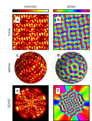
SUPP. FIG. 1: The intensity (modulus squared) and phase (argument) of sample random energy eigenfunctions in 2D systems. a-b square with periodic boundary conditions (flat 2-torus); c-d the 2-sphere; e-f the 2D harmonic oscillator (2DHO). These are found using 2D analogues of (1), i.e. complex random superpositions with the same energy (spatial frequency) of 2D plane waves in a and b, spherical harmonics in c and d, and 2D harmonic oscillator eigenstates (Hermite-Gauss functions) in e and f.

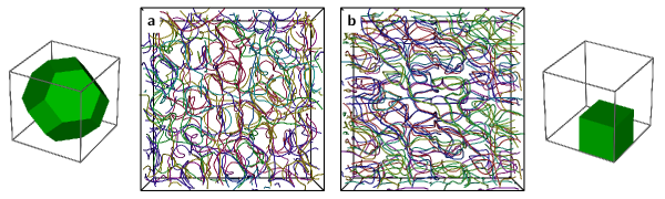
SUPP. FIG. 2: Vortices in random energy eigenfunctions in a periodic cubic cell; a without and b with the additional constraint to octant symmetry. In a, $\ell^{2}+m^{2}+n^{2}=26$ and the periodic unit cell of the vortex tangle is the truncated octahedron. In b, $\ell^{2}+m^{2}+n^{2}=27=3\times 3^{2}$ and the additional symmetry due to all $\vec{k}$ components being odd means that the periodic unit cell of the vortex tangle is an octant of field’s primitive cubic cell.

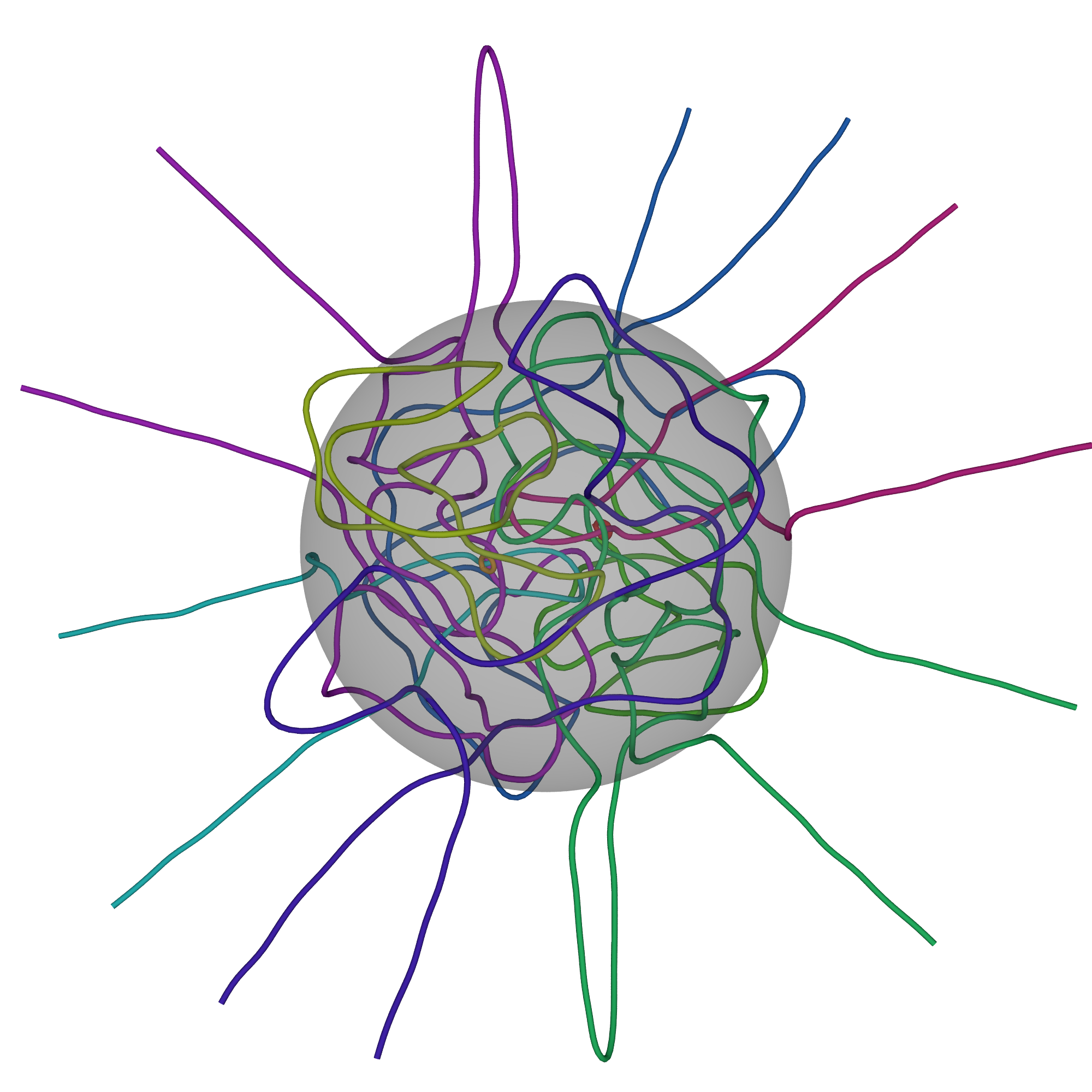
SUPP. FIG. 3: Vortices in a random eigenfunction of the 3DHO with N=8. The grey region marks the classical volume where the energy is greater than the potential, and which effectively bounds the vortex tangle; vortices become straight lines as they move further from this shell.

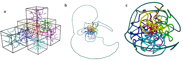
SUPP. FIG. 4: Projections of the 3-sphere to 3-dimensional Euclidean space, illustrated with the vortices of a random eigenfunction with $N=7$. a shows the vortices in each octant of a net of the 3-sphere (i.e. a discontinuous map, with the geometry recovered by joining cubic cells along their faces). The vortices within each such octant are given a different colour. In b the same vortices are shown via stereographic projection, continuous and angle preserving but significantly distorting distances, with the vortices still coloured according to the octants they passed through in a. c shows the rescaled stereographic projection used in Figures 1, 3 and 4 of the main text.

In each system, we compute the total vortex length per random eigenfunction. The distribution of these total lengths is found to be numerically strongly peaked at a value given by the integral over the volume of the mean vortex density, which is analogous to calculations of nodal lengths for real random eigenfunctions berry02 ; rudnick08 ; gnutzmann14 ; wigman09 ; bies2002 (the width of the distribution is in each case proportional to the square root of the reciprocal of the degeneracy). Significantly, this total line length is proportional to the systems’ total energy $E_{N}$. This justifies our comparison in the main text, of energy against knotting probability and complexity, as this provides a physical measure of the total arc length in each tangle. The reference wavelength $\lambda$ in the main text is proportional to $E_{N}^{-1/2}$. In all cases, we estimate the numerical error in the calculated total arclength (including that on smoothing the sampled curves) to be no bigger than $5\%$. Decreasing this would require significantly higher resolution in the sampling, and of course would not affect the topological results.

The vortex density in the ideal isotropic complex RWM is well known to be $2ME/3\pi\hbar^{2}$ F ; G . The other systems approach this limit when $N\gg 1$, but in slightly different ways. The vortex density in the periodic 3-cell depends weakly on direction U , but at the values of $N$ considered here can be taken to be the isotropic density. The density in the 3-sphere is constant, and can be found using standard methods to be $E_{N}/3\pi=N(N+2)/3\pi$ (as above, ignoring physical constants and assuming a 3-sphere of unit radius), consistent with the isotropic random wave model result. The vortex density of the 3DHO is the most complicated, as the density is inhomogeneous and isotropic (depending on the value of the radius), and we omit detailed calculations here. Although the detailed results depend subtly (although not strongly) on $N$, the total arclength we calculate (truncating at twice the classical radius) is indeed found to be proportional to the total energy within comparable error.

In the results of the main text (including Figures 1 and 2), the calculations involved the 3-torus with $N=9$, with average total arclength approximately $$2000$~{}\lambda$; the 3-sphere with $N=17$ and average arclength approximately $$1930$~{}\lambda$; and the 3DHO with $N=21$ and average arclength approximately $$1830$~{}\lambda$. Although these are not exact matches, they are sufficiently close to compare topological statistics which are representative of general trends.

Supplementary Note 2:
Numerical techniques

Vortex lines are numerically tracked in 3D complex wavefunctions via a recursively resampled Cartesian grid method (RRCG). The core procedure follows previous numerical experiments vachaspati84 ; caradoc-davies99 ; Y , sampling the field at points on a 3D Cartesian grid and searching for local 2D grid plaquettes that are penetrated by a vortex. Vortices can be located in this 2D problem either via their intensity (which must be zero) or the circulation of their phase (which must be $2\pi$ in a path around the edge of a penetrated plaquette). It is standard to make use of this latter property, as zeros of the intensity are difficult to pinpoint numerically whereas the integrated total change of the phase can be detected even with relatively few sample points situated far from the vortex core; in fact, it is possible to detect most vortex penetrations with just the four sample points at the corners of grid plaquettes with side length around $0.1\lambda$.

A vortex line is additionally oriented by the right-handed sense of its quantised phase circulation, and according to this orientation must both enter and leave any grid cell that it passes through (it cannot simply terminate). The above procedure therefore normally detects the passage of a vortex through two different faces of each 3D grid cell. The vortex curve is recovered by joining these points and connecting each line segment with those in neighbouring cells to build up a piecewise-linear approximation to the three-dimensional vortex tangle.

This basic procedure does not perfectly detect vortex curves; vortex penetration of a 2D plaquette may not be detected if the local phase change is too anisotropic on the scale of the lattice spacing. This occurs especially when the lattice spacing is large, or if vortices approach closely, since in this case the $2\pi$ integrated phase about multiple vortices cannot be distinguished from the zero phase change which would mean a vortex is not present. Such problems give apparently discontinuous vortex lines, and the numerical procedure resamples the complex wavefield in the cells around these apparent discontinuities, generating a new local grid with higher resolution and repeating the search for vortices using this new lattice. If a vortex is discontinuous on the new grid, the resampling procedure is repeated recursively, and is guaranteed to terminate eventually since at very small lengthscales the smoothness of the field limits large phase fluctuations. By matching the different numerical lattices with one another and joining vortices where they pass between them, the recovered vortex curves are continuous within the full numerically sampled region, forming locally-closed loops or terminating on its boundaries. A primary advantage of this method is that it correctly resolves the local topology of vortex lines without requiring a prohibitively high resolution sampling over the entire field. This issue has alternatively been addressed in previous studies using physical arguments Y , an extra random choice vachaspati84 or a different grid shape hindmarsh95 , but none of these options is so numerically convenient while guaranteeing robust results. The resampling procedure can also be used to enhance the recovery of local vortex geometry, as described in U , but this is not important to the topological results described here.

The RRCG algorithm must further be modified in each of the three different systems of wave chaos we consider. With periodic boundary conditions, the finite numerical grid is itself made periodic along each Cartesian axis of the periodic cell, but the RRCG procedure is otherwise unaffected. Vortex loops are recovered by ‘unwrapping’ vortex segments through the periodic boundaries, equivalent to tiling space with periodic cells and following each loop continuously until its starting point, so the net vortex loop can (and often does) pass through several periodic cell.

In the harmonic oscillator, vortices may extend to infinity and we only consider vortex length within a finite radius of the origin. As distance from the origin increases beyond the classical radius, vortex curves tend to radial lines without further tangling (clearly visible in Supplementary Figure 3, or Figure 1 of the main text), and we take the cutoff at twice the classical radius $\sqrt{2E}$.

Tracking vortices in the 3-sphere is more complicated since it must be projected to flat real space to make it accessible to our 3D Cartesian grid based numerical method. Standard methods such as stereographic projection are numerically inefficient because they greatly distort distances and therefore vortex densities, such that an initial numerical resolution sufficient to detect vortices in the densest regions will be far higher than necessary in other areas where the vortex densities are lower. We instead divide the 3-sphere into a net of eight cubes, with each taken to be a Cartesian grid covering one of the eight octants of the 3-sphere. The RRCG algorithm is run on each octant grid, with overall topology recovered by identification of faces in the overall net. This process is illustrated in Supplementary Figure 4, where 4a shows vortices in each of the cubic octants of the net, discontinuous where they meet the octant faces, while 4b-c show the same vortices in two continuous projections to $\mathbb{R}^{3}$; these are respectively stereographic projection and the projection used in the main text. Although the spatial round metric of the 3-sphere does vary over each octant, the length variation is in fact relatively small (by no more than a factor of $2$) and does not significantly impede vortex tracking efficiency.

Supplementary Note 3:
Topological background and techniques

The analysis of topology in wave chaos requires that the topological knot type of each vortex curve can be distinguished. It is standard to accomplish this through the calculation of knot invariants, which are mathematical objects (integers, polynomials, …) that can be computed from the geometric conformation but are the same for all representations of the same topological knot (i.e. under ambient isotopy). Mathematical knot theory provides many such invariants, which have been used to develop a taxonomy summarised in knot tables, although no invariant is known to distinguish all knots. The values of invariants associated with the unknot (i.e. a loop which is not knotted) are usually trivial, whereas the invariants of proper knots usually take other values. Knot tables are usually ordered by the invariant minimal crossing number, i.e. according to the smallest number of crossings the knot admits on projection into a 2-dimensional plane; the first few prime knots are written $3_{1}$ (the only knot with minimal crossing number 3, i.e. the trefoil knot), $4_{1}$ (the only knot with minimal crossing number 4, i.e. the figure-8 knot), then $5_{1},5_{2}$, and so on. Supplementary Figure 5 shows the 35 non-trivial prime knots with 8 or fewer minimal crossings. Composite knots, those which can be separated into distinct prime knot components each with smaller minimal crossing number such as Figure 1e in the main text, are not included in this table. Composite knots are referred to as combinations of prime knots joined by $\#$, or by exponents for a repeated component; for instance, $3_{1}^{2}$ for the double trefoil knot or $3_{1}\#4_{1}$ for the join of the first two non-trivial knots. Invariants of composite knots can usually be factorised in some sense into those of the component knots, and they are denoted by adjoining the notation of their prime components. Whether a given vortex curve is knotted is found by calculating one or more knot invariants, and then looking these up in the knot table. The values of invariants can also give information about different families and classes of which a given knot is a member X ; knotinfo .

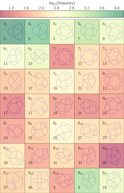
SUPP. FIG. 5: The first 35 non-trivial prime knots, ordered by minimal crossing number. These are all the prime knots with 8 or fewer crossings in their minimal projection, with the standard name of the knot ($3_{1}$, $4_{1}$, etc) in the top left. The value of the knot determinant $|\Delta(-1)|$ for each knot is also given in the lower left of each cell; of these, none has the same determinant as the unknot (which is unity). The cells are coloured according to the $\log$ of its frequency of occurrence in all of our data (unnormalised, and taken over across all systems at various different energies), as detected by the Alexander polynomial at roots of unity. This figure includes a small number of incorrect identifications; the knots $8_{20}$ and $8_{21}$ are surprisingly common here, but this is because their Alexander polynomials are equal to those of the more common composite knots $3_{1}^{2}$ and $3_{1}\#4_{1}$ (not depicted). These misidentifications would be corrected by the hyperbolic volume or Vassiliev invariants, which are not applied here. The image of each knot is from the KnotInfo Table of Knot Invariants knotinfo , and the invariant values from KnotInfo and the Knot Atlas X .

Our primary requirement is to distinguish lines that are knotted from those that are not, and to be able to sort knotted curves by some simple knot invariant which measures their complexity. For this we employ the Alexander polynomial G $\Delta(t)$, which is straightforward to calculate up to an unknown factor of $t^{n}$ k (e.g. the unknot has Alexander polynomial $\Delta(t)=t^{n}$, the trefoil knot $3_{1}$ has $\Delta(t)=(1-t+t^{2})t^{n}$) as the determinant of a matrix with dimension $n-1$ for projection of the knot with $n$ crossings. Some knotted curves have Alexander polynomial $\Delta(t)=t^{n}$, like the unknot, but such knots are comparatively rare; the simplest examples are two knots with minimal crossing number 11, already complex enough to be highly uncommon in eigenfunction vortex tangle. Supplementary Figure 5 demonstrates this trend; each knot is coloured by the frequency of its occurrence across all eigenfunction data in all different systems, with most knots by frequency having low minimal crossing numbers, and those with $8$ crossings already being up to $1000$ times less common.

Since the projections of curves in our numerical tangle may have several thousand crossings (even after algorithmic simplification), it can be impractical to calculate the full Alexander polynomial symbolically. Thus we evaluate the Alexander polynomial at specific values, conveniently the first three nontrivial roots of unity, $-1$ (giving the knot determinant k ), $\exp(2\pi i/3)$ and $i$. The absolute value $|\Delta(t)|$ is invariant under this substitution regardless of the unknown factor of $t$, and this combination of integer values discriminates the tabulated knots almost as well as the symbolic Alexander polynomial itself; for instance, they are equally discriminatory when distinguishing the 802 prime knots with 11 or fewer crossings. The determinant is a commonly used tool for identifying knots in numerical studies moore04 ; k , although we have not found $\Delta$ at other roots of unity used elsewhere in numerical knot identification.

The knot determinant is also convenient on its own as a measure of knot complexity; it takes its minimum value on the unknot, $\Delta(-1)=1$, and tends to increase with crossing number (we find it appears on average linearly related to the exponential of the minimal crossing number, consistent with known bounds stoimenow2003 ), and for a composite knot is the product of determinants of its prime components soteros92 . Many other invariants fulfil these conditions, but the determinant is convenient due to its ease of calculation, the same reason that it is used already in knot detection. Supplementary Figure 5 includes this complexity trend for each of the non-trivial knots with 8 or fewer minimal crossings, taking values from $3$ (for the simple trefoil knot $3_{1}$) to $45$ (for $8_{18}$).

Where it is necessary to distinguish the knot type beyond the discriminatory ability of the Alexander polynomial, such as in Figure 1 of the main text, further invariants are used. Modern knot theory supplies many powerful options, but most of these are impractical to calculate rapidly for large numbers of geometrically complex projections (being calculable only in exponential time), and we instead use more efficient options that are nevertheless sufficient. First, the Vassiliev invariants of order two and three are also integer invariants of knots, practically calculable in square or cubic time respectively in the number of crossings of a given diagram, but adding further discriminatory power beyond that of the Alexander polynomial W . These invariants have been used previously in numerical knot identification moore04 . We also use the hyperbolic volume, which takes values in the real numbers and is nonzero only for the so-called hyperbolic knots, but is highly discriminatory among this class, and for this reason has seen major use in knot tabulation hoste1998 . Most tabulated prime knots are hyperbolic (of the the 1.7 million prime knots with 16 or fewer crossings, only 32 are not hoste1998 ), but composite knots always have volume zero and so are also readily separated from prime knots in this way. The hyperbolic volume is calculated using the standard topological manifold routines in SnapPy V , which return only an approximation but are reliable over the range of complexities we address.

Neither these Vassiliev invariants nor the hyperbolic volume are perfect knot invariants, but combined with the Alexander polynomial they are sufficiently discriminatory to unambiguously identify most simple knots where necessary, such as those in Figures 1 and 4 of the main text. They also further verify that in practice the Alexander polynomial rarely fails to detect knotting among the vortex lines of our eigenfunction systems, as those prime knots with $\Delta$ indistinguishable from the unknot are generally easily detected to be hyperbolic.

Supplementary Note 4:
Symmetries of knots

Some aspects of knotting in eigenfunctions are dominated by the symmetry of the system. Such symmetries have already been removed in our analysis of wave chaos under periodic boundary conditions, but remain in the eigenfunctions of both the 3-sphere and 3DHO.

In the 3-sphere, all eigenfunctions satisfy the condition $\Psi(\psi,\theta,\phi)=(-1)^{N}\Psi(\pi-\psi,\pi-\theta,\phi+\pi)$ and, since, vortices are nodal lines, a vortex at a given position is always paired with a vortex at its 3-sphere antipode. If these points are on different vortex lines then both lines are identical up to a rotation of the 3-sphere by $\pi$ through some plane in four dimensions, and so they have the same knot type. If two antipodal points are positions on the same vortex line then the entire vortex curve must be symmetric (carried to itself) under this rotation. Not all knot types can meet this geometric constraint; those that can do so are a subclass of knots that are strongly amphicheiral.

Strong amphicheirality is an extension of the more commonly considered chirality of knots; a knot is chiral if it is not equivalent to its mirror image (i.e. with the overstrand and understrand at each crossing switched), and otherwise is called amphicheiral (or equivalently achiral). Both types are common, e.g. the trefoil knot is chiral (shown in Supplementary Figure 6a), but the next non-trivial knot, $4_{1}$, is amphicheiral adams94 (evident in the projection of Supplementary Figure 6c, equal to its mirror image under a rotatation by $\pi$ about the marked point, discussed further below). Strong amphicheirality additionally demands that the knot be equivalent to its mirror not just in its knot type, but under a specific involution of the 3-sphere, i.e. a geometric transformation that is its own inverse kawauchi96 . Supplementary Figure 6b-d shows three example diagrams of strongly amphicheiral knots in which the involution is rotation in two dimensions by $\pi$ about the marked point, which in each case takes the knot diagram to its mirror image; b gives an example of how any composite of a knot with its mirror image admits a strongly amphicheiral conformation kawauchi96 , c shows strong amphicheirality of the knot $4_{1}$, and d the same for the more complicated $10_{99}$.

Strongly amphicheiral knots are additionally split into two classes depending on how the involution affects the orientation of the curve, which for an arbitrary curve may not matter but in vortex lines is fixed by the orientation of the phase. A knot is strongly negatively amphicheiral if this orientation is preserved under the involution, or strongly positively amphicheiral if its orientation is reversed. Supplementary Figure 6b and 6c show strongly negatively amphicheiral examples (note the reversal of the marked orientation under rotation about the marked point), and this is additionally the reason for these diagrams being drawn as open curves closing at infinity; under the involution of rotation, the origin of rotation is privileged such that the curve must pass through this point and close at infinity (equivalent to the antipode considered on the 3-sphere). No other conformation would be able to meet the strong negative amphicheiral symmetry. In contrast, Supplementary Figure 6d shows a strong positive amphicheiral conformation of the knot $10_{99}$. In fact, $10_{99}$ is the simplest knot with strong positive amphicheiral symmetry, and (with a different conformation) also supports strong negative amphicheirality.

In eigenfunctions of the 3-sphere, the symmetry under rotation reverses the local vortex line orientation according to its phase circulation. This means that such vortices passing through antipodal points can only form strong positive amphicheiral knots, of which the simplest example is the unknot but the first non-trivial prime example is $10_{99}$. Although not discussed in the main text, this knot and others with the same symmetry occur with disproportionate frequency in 3-sphere eigenfunctions, with simpler knots occurring only as symmetric antipodal pairs (under the eigenfunction symmetry) or as strong positive amphicheiral composite knots. This symmetry also has an equivalent effect at all $N$, and so does not lead to significant patterns in knotting probability with energy, as can be seen in Figure 3a of the main text.

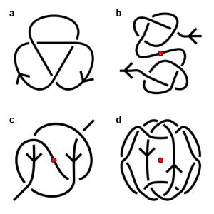
SUPP. FIG. 6: Knots exhibiting different symmetries. In a a trefoil knot, which is chiral and cannot be transformed to its mirror image without passing the curve through itself. b-d show strongly amphicheiral conformations of three other knots, equivalent to their mirror images under a rotation by $\pi$ about the marked red point, and with or without an orientation reversal of the line; in b a strongly negatively amphicheiral composite double trefoil knot ($3_{1}^{2}$), in c a strongly negatively amphicheiral figure-eight knot ($4_{1}$), and in d a strongly positively amphicheiral knot $10_{99}$.

Eigenfunctions of the 3DHO have a similar symmetry under inversion through the origin, $\Psi(\vec{r})=(-1)^{N}\Psi(-\vec{r})$, but with the difference now that this supports only strong negative amphicheiral symmetry; the vortex tangent direction is preserved under the inversion. As with the 3-sphere, any vortex line passing through $\vec{r}$ is paired with one at $-\vec{r}$, and if these points are on different vortices then the entire vortex line appears twice. If the points are on the same vortex line then it must take up a strongly negatively amphicheiral conformation. Under inversion, the only way to do so while meeting the symmetry of the eigenfunction is to pass through the origin and to close at infinity, taking a conformation such as those in Supplementary Figure 6b and 6c. Unlike in the 3-sphere, only one vortex line in a given eigenfunction can do so, and at most one strongly amphicheiral knot can appear. Since the 3DHO naturally supports vortex lines which eventually extend to infinity in straight lines outside the classical radius, it is possible for the privileged origin vortex line to do so and to be knotted.

The probability of a vortex passing through the origin depends directly on $N$; when $N$ is even, random degenerate eigenfunctions are non-zero at the origin, whereas when $N$ is odd the origin is always a nodal point and sits on a vortex line. This is the reason for the observed odd-even discrepancy in knotting probability with energy in Figure 3 of the main text; when $N$ is even there is no strongly negatively amphicheral vortex line and all knots occur in pairs of antipodal mirrors. When $N$ is odd, such a vortex line always exists and can form a strongly negatively amphicheiral conformation of a knot. This is relatively common, as the total arclength required to form such a knot is often lower than for the two symmetric copies otherwise required. This knot is frequently prime (unlike with strong positive amphicheirality, there are several strongly negatively amphicheiral knots with fewer than 10 crossings), but can also be a composite of a knot with its mirror image. Compatible knots are thus overrepresented in the statistics of knot type within the system, but now only when $N$ is odd explaining the strong parity dependence of knotting in the 3DHO. The effect is also strong enough to persist even at $N$ high enough that there is a 50% or higher chance for one or more pairs of the other vortex lines in a given eigenfunction to form knots.

References

- (1) M V Berry “Regular and irregular semiclassical wavefunctions” J Phys A 10 2083-91 (1977)
- (2) H-J Stöckmann Quantum Chaos: an introduction Cambridge University Press (2006)
- (3) E Madelung “Quantentheorie in hydrodynamischer Form” Z Phys 40 322-6 (1927)
- (4) J O Hirschfelder, C J Goebel & L W Bruch “Quantized vortices around wavefunction nodes. II.” Journal of Chemical Physics 61 5456-9 (1974)
- (5) J Riess, “Nodal structure, nodal flux fields, and flux quantisation in stationary quantum states” Phys Rev D 2 647-53 (1970)
- (6) J F Nye & M V Berry “Dislocations in wave trains” Proceedings of the Royal Society 336 165-90 (1974)
- (7) C N Weiler, T W Neely, D R Scherer, A S Bradley, M J Davis & B P Anderson “Spontaneous vortices in the formation of Bose-Einstein condensates” Nature 455 948-51 (2008)
- (8) M R Dennis and K O’Holleran and M J Padgett “Singular Optics: Optical Vortices and Polarization Singularities”, in Progress in Optics volume 53 (E Wolf, ed) Elsevier, 2009, pp 293-363
- (9) C F Barenghi “Knots and unknots in superfluid turbulence” Milan J Math 75 177-96 (2007)
- (10) A Nahum, J T Chalker, P Serna, M Ortuño & A M Somoza “Length distributions in loop soups” Physical Review Letters 111 100601 (2013)
- (11) A Vilenkin and E P S Shellard Cosmic Strings and Other Topological Defects Cambridge University Press (1994)
- (12) K O’Holleran, M R Dennis, F Flossmann & M J Padgett “Fractality of light’s darkness” Physical Review Letters 100 053902 (2008)
- (13) D Kleckner & W T M Irvine “Creation and dynamics of knotted vortices” Nature Physics 9 253-8 (2013)
- (14) U Tkalec, M Ravnik, S C̆opar, S Z̆umer & I Mus̆evic̆ “Reconfigurable knots and links in chiral nematic colloids” Science 333 62-5 (2011)
- (15) B Senyuk, Q Liu, S He, R D Kamien, R B Kusner, T C Lubensky & I I Smalyukh “Topological colloids” Nature 493 200-5 (2013)
- (16) M R Dennis, R P King, B Jack, K O’Holleran & M J Padgett “Isolated optical vortex knots” Nature Physics 6 118-21 (2010)
- (17) D Kleckner, L H Kauffman and W T M Irvine “How superfluid vortex knots untie” Nature Physics doi:10.1038/nphys3679 (2016)
- (18) M V Berry “Knotted zeros in the quantum states of hydrogen” Found Phys 31 659-67 (2001)
- (19) M V Berry and M R Dennis “Knotted and linked phase singularities in monochromatic waves” Proc R Soc A 457 2251-63 (2001)
- (20) R J Adler, O Brobowski, M S Borman, E Subag & S Weinberger “Persistent homology for random fields and complexes” Institute of Mathematical Statistics Collections 6 124-42 (2010)
- (21) M V Berry & M R Dennis “Phase singularities in isotropic random waves” Proceedings of the Royal Society A 456 2059-79 (2000)
- (22) A C White, C F Barenghi, N P Proukakis, A J Youd & D H Wacks “Nonclassical velocity statistics in a turbulent atomic Bose-Einstein Condensate” Physical Review Letters 104 075301 (2010)
- (23) D Rolfsen Knots and Links American Mathematical Society (2004)
- (24) D Bar-Natan The Knot Atlas http://katlas.org (January 2016)
- (25) A J Taylor & M R Dennis “Geometry and scaling of tangled vortex lines in three-dimensional random wave fields” Journal of Physics A 47 465101 (2014)
- (26) E Orlandini & S G Whittington “Statistical topology of closed curves: some applications in polymer physics” Reviews of Modern Physics 79 611-42 (2007)
- (27) M Culler, N M Dunfield & J R Weeks SnapPy, a computer program for studying the topology of 3-manifolds, http://snappy.computop.org (January 2016)
- (28) N T Moore, R C Lua & A Y Grosberg “Topologically driven swelling of a polymer loop” Proceedings of the National Academy of Sciences 101 13431-5 (2004)
- (29) M Polyak & O Viro “Gauss diagram formulas for Vassiliev invariants” International Mathematics Research Notices 11 445-53 (1994)
- (30) K O’Holleran, M R Dennis, & M J Padgett “Topology of light’s darkness” Physical Review Letters 102 143902 (2009)
- (31) J M van Buskirk “A class of negative-amphicheiral knots and their Alexander polynomials” Rocky Mountain Journal of Mathematics 13 413-22 (1983)
- (32) K Koniaris & M Muthukumar “Knottedness in ring polymers” Physical Review Letters 66 2211-4 (1991)
- (33) A Enciso, D Hartley & D Peralta-Salas “A problem of Berry and knotted zeros in the eigenfunctions of the harmonic oscillator” Preprint at http://arxiv.org/abs/1603.03214 (2015)
- (34) A Enciso, D Hartley & D Peralta-Salas “Dislocations of arbitrary topology in highly excited states of the hydrogen atom” Preprint at http://arxiv.org/abs/1603.03214 (2016)
- (35) M V Berry “Faster than Fourier”, in Quantum Coherence and Reality; in celebration of the 60th Birthday of Yakir Aharonov (J S Anandan and J L Safko, eds) World Scientific, Singapore, 1994, pp 55-65
- (36) G Blum, S Gnutzmann & U Smilansky “Nodal domain statistics: a criterion for quantum chaos” Physical Review Letters 88 114101 (2002)
Acknowledgments
The authors thank Michael Berry for valuable discussion and for originally proposing the problem investigated here, and Andrea Aiello, Stu Whittington, Daniel Peralta-Salas and Dmitry Jakobson for useful suggestions. This research was funded by a Leverhulme Trust Research Programme Grant. This work was carried out using the computational facilities of the Advanced Computing Research Centre, University of Bristol. The authors are grateful to the KITP for hospitality during the early part of this work. Alexander Taylor was partially funded by the Engineering and Physical Sciences Research Council and Mark Dennis by the the Royal Society of London.

References

- (1) M V Berry & M R Dennis “Phase singularities in isotropic random waves” Proceedings of the Royal Society A 456 2059-79 (2000)
- (2) A C White, C F Barenghi, N P Proukakis, A J Youd & D H Wacks “Nonclassical velocity statistics in a turbulent atomic Bose-Einstein Condensate” Physical Review Letters 104 075301 (2010)
- (3) A J Taylor & M R Dennis “Geometry and scaling of tangled vortex lines in three-dimensional random wave fields” Journal of Physics A 47 465101 (2014)
- (4) H Hochstadt The Functions of Mathematical Physics Wiley Interscience (1971)
- (5) A I M Rae Quantum Mechanics CRC Press 5th edition (2007)
- (6) M V Berry “Statistics of nodal lines and points in chaotic quantum billiards: perimeter corrections, fluctuations, curvature” J Phys A 35 3025-38 (2002)
- (7) Z Rudnick & I Wigman “On the volume of nodal sets for eigenfunctions of the Laplacian on the torus” Annales Henri Poincaré 9 109-30 (2008)
- (8) S Gnutzmann & S Lois “Remarks on nodal volume statistics for regular and chaotic wave functions in various dimensions” Phil Trans Roy Soc Lond A 372 20120521 (2014)
- (9) I Wigman “On the distribution of the nodal sets of random spherical harmonics” J Math Phys 50 013521 (2009)
- (10) W E Bies & E J Heller “Nodal structure of chaotic eigenfunctions” J Phys A 35 5673-85 (2002)
- (11) D Rolfsen Knots and Links American Mathematical Society (2004)
- (12) E Orlandini & S G Whittington “Statistical topology of closed curves: some applications in polymer physics” Reviews of Modern Physics 79 611-42 (2007)
- (13) K O’Holleran, M R Dennis & M J Padgett “Fractality of light’s darkness” Phys Rev Lett 102 143902 (2009)
- (14) K O’Holleran, M R Dennis, F Flossmann & M J Padgett “Fractality of light’s darkness” Physical Review Letters 100 053902 (2008)
- (15) T Vachaspati & A Vilenkin “Formation and evolution of cosmic strings” Phys Rev D 30 2036-45 (1984)
- (16) B M Caradoc-Davies, R J Ballagh & K Burnett “Coherent dynamics of vortex formation in trapped Bose-Einstein condensates” Phys Rev Lett 83 895-8 (1999)
- (17) M Hindmarsh & K Strobl “Statistical properties of strings” Nucl Phys B437 471-88 (1995)
- (18) D Bar-Natan The Knot Atlas http://katlas.org (January 2016)
- (19) J C Cha & C Livingston KnotInfo: Table of Knot Invariants, http://www.indiana.edu/k̃notinfo (January 2016)
- (20) N T Moore, R C Lua & A Y Grosberg “Topologically driven swelling of a polymer loop” PNAS 101 13431-35 (2004)
- (21) A Stoimenow “On the coefficients of the link polynomials” Manuscripta Math 110 203-36 (2003)
- (22) C E Soteros, D W Sumners & S G Whittington “Entanglement complexity of graphs in ” Math Proc Camb 111 75-91 (1992)
- (23) M Polyak & O Viro “Gauss diagram formulas for Vassiliev invariants” International Mathematics Research Notices 11 445-53 (1994)
- (24) J Hoste, M Thistlethwaite & J Weeks “The first 1,701,935 knots” Math Intelligencer 20 (1998)
- (25) M Culler, N M Dunfield & J R Weeks SnapPy, a computer program for studying the topology of 3-manifolds, http://snappy.computop.org (January 2016)
- (26) C C Adams The Knot Book American Mathematical Society (1994)
- (27) A Kawauchi A Survey of Knot Theory Birkhäuser (1996)