Least worst regret analysis for decision making under uncertainty,
with applications to future energy scenarios

Abstract

Least worst regret (and sometimes minimax) analysis are often used for decision making whenever it is difficult, or inappropriate, to attach probabilities to possible future scenarios. We show that, for each of these two approaches and subject only to the convexity of the cost functions involved, it is always the case that there exist two “extreme” scenarios whose costs determine the outcome of the analysis in the sense we make clear. The results of either analysis are therefore particularly sensitive to the cost functions associated with these two scenarios, while being largely unaffected by those associated with the remainder. Great care is therefore required in applications to identify these scenarios and to consider their reasonableness.

We also consider the relationship between the outcome of a least worst regret and a Bayesian analysis, particularly in the case where the regret functions associated with the scenarios largely differ from each other by shifts in their arguments, as is the case in many applications.

We study in detail the problem of determining an appropriate level of electricity capacity procurement in Great Britain, where decisions must be made several years in advance, in spite of considerable uncertainty as to which of a number of future scenarios may occur, and where least worst regret analysis is currently used as the basis of decision making.

1 Introduction

Many economic decisions, for example that of an appropriate level of investment, need to be taken in the face of uncertainties about future conditions. Were these conditions known an optimal decision might be made, usually on the basis of the minimisation of a cost function. Indeed were it possible to assign probabilities to future conditions—frequently condensed into a finite number of scenarios—one might reasonably minimise an expected cost, or perhaps some other appropriate functional of the probability distribution of cost (see, for example, Berger [1]). However, even this is frequently not possible, either because of insufficient data or other information with which to make an appropriate assessment of probabilities, or because future conditions are dependent upon other human decisions—for example political decisions—yet to be made, and it would be inappropriate to attempt to second-guess these.

A Bayesian decision maker would simply assign subjective probabilities to future scenarios, using such information as was available, and then proceed as above. However, there is often an understandable reluctance to do this, and then recourse is made to one of various economic decision making criteria which do not require the assignment of probabilities, and which are therefore often described as “robust”. Whether this really makes sense is a matter of philosophical debate: if one believes that the probabilities matter—at least, for example, that highly likely future scenarios should have more weight in the decision making process than highly unlikely ones—then the use of techniques which entirely ignore probabilities might simply be regarded as suboptimal. However, the continued use of such techniques is often justified on pragmatic grounds.

In the present paper, we study two commonly used non-probabilistic techniques. In both cases associated with each future scenario to be considered is a cost function defined on the set of possible decisions. In minimax analysis that decision is made which minimises the maximum cost to be incurred over all possible scenarios. This technique, based on extreme risk aversion, has a long history; for an early systematic treatment, see Savage [2]. In least worst regret (or minimax regret) analysis, the cost function associated with each scenario is modified by subtracting its minimum value over the decision set; the resulting functions are termed the regret functions associated with the scenarios, and the minimax criterion is applied to the set of regret functions rather than the original cost functions. This technique was first introduced in the early 1980s, independently in the papers by Loomes and Sugden [3] and by Bell [4] and in the book by Fishburn [5], and has been the subject of some subsequent study, usually in the context of specific and often complex models.

More formal definitions of both these techniques are given in the next section. Least worst regret analysis in particular is much used in practice. However, depending on the nature of the cost functions involved, neither technique can be said to be always scientifically rational. Minimax analysis suffers from the problem that a single scenario with an associated cost function which is uniformly high across the decision set (notably one which is pointwise higher than the cost functions associated with all other scenarios) may alone determine the outcome of the analysis, even though this scenario may be unlikely and/or may have a relatively flat cost function—note that either of the latter circumstances strongly suggests that such a scenario should not be influential in cost-based decision making. Least worst regret analysis avoids this particular problem by effectively adjusting the cost function associated with each scenario so that its minimum value across the decision set is zero (thus defining the regret function). There are some well-rehearsed arguments as to why this is to be preferred—see, for example, the references cited above, and note also that a Bayesian probabilistic analysis also depends on the cost functions only through their associated regret functions, as noted more formally in the next section. However least worst regret analysis has the unfortunate property that, depending on the cost functions involved, which of two decisions is to be preferred may depend on the costs associated with a third possible decision—-or indeed on whether that third possible decision is actually included in the decision set—a point to which we return in more detail in Section 2. Neither minimax analysis nor a Bayesian probabilistic analysis suffers from this problem.

Thus we would argue that the uncritical adoption of either of the above techniques is to be avoided. Whether either of them works well in practice depends very much on the shape of the cost functions involved, as well as on the specification of the decision set itself. This is one issue we wish to explore in the present paper. Our particular interest is in least worst regret analysis, as the latter seems to be presently widely used. One such use is that of the determination, in Great Britain, of an optimal level of provision of “conventional” electricity generation capacity; this is something which must be decided several years in advance, even although there are considerable uncertainties as to both future electricity demand and the future availability of “non-conventional”, i.e. renewable, generation. We study this example in Section 4.

In Section 2 we give more formal definitions and study some relevant mathematical properties of both minimax and least worst regret analysis. Our main result is that in either case, given the convexity of the cost functions, it is possible to identify two “extreme” scenarios which essentially determine the outcome of the analysis in a sense we make precise there—roughly speaking the other scenarios do not matter at all provided none of them becomes more extreme than the two above. It follows that great care needs to be taken in the specification of the most “extreme” scenarios to be considered. We also study the common situation in which, at least to a first approximation, the differences between the scenario regret functions are represented by shifts in their arguments; here the “extreme” scenarios are immediately identifiable and the properties of a least worst regret analysis—particularly robustness with respect to scenario variation—readily understood. Finally in that section, we consider briefly the alternative Bayesian analysis and how the outcome of a least worst regret analysis might relate to it.

Section 3 studies the problem in which each of the scenario cost functions is—again at least approximately—the sum of an exponentially decaying and a linearly increasing term. Here it is possible to make quite quantitative deductions about the outcome of a least worst regret analysis and its relation to that of possible Bayesian analyses. This situation is common when the decision problem is that of choosing an appropriate level of investment—in the face of future uncertainty—so as to manage risk. It is in particular the case (again to a good approximation) for the Great Britain electricity capacity procurement problem which was introduced above and which is studied in detail in the following section.

In the concluding Section 5 we make some further brief comments about the sensible application of least worst regret analysis.

2 Minimax and least worst regret analysis

Both minimax and least worst regret (LWR) analysis are defined in relation to a set $\mathcal{S}$ of scenarios—which in the present note we take to be finite—and a set $\mathcal{D}$ of possible decisions. The decision set $\mathcal{D}$ may be finite or infinite. Corresponding to each scenario $i\in\mathcal{S}$ is a cost function $f_{i}$ defined on the set $\mathcal{D}$ such that for each $x\in\mathcal{D}$ the quantity $f_{i}(x)$ is the cost associated with the decision $x$ under the scenario $i$. The decision problem is that of choosing $x\in\mathcal{D}$ such that the associated costs $f_{i}(x)$ are in some sense minimised. This problem as stated is not yet well-defined, and our interest is the mathematical properties and relationships between the various rival approaches to making it well-defined, in particular with the minimax, least worst regret and Bayesian approaches (where the latter additionally requires an assignment of probabilities to scenarios).

We shall find it convenient to think also of the decision problem associated with any subset $\mathcal{S}^{\prime}$ of the set of scenarios $\mathcal{S}$. For any such subset $\mathcal{S}^{\prime}$, define further the maximum cost function $f_{\mathcal{S}^{\prime}}$ by

$$f_{\mathcal{S}^{\prime}}(x)=\max_{i\in\mathcal{S}^{\prime}}f_{i}(x).$$ (1)

Then the minimax solution $x^{*}_{\mathcal{S}^{\prime}}$ to the decision problem associated with the set $\mathcal{S}^{\prime}$ is the value of $x$ within the decision set $\mathcal{D}$ which minimises $f_{\mathcal{S}^{\prime}}(x)$. In particular $x^{*}_{\mathcal{S}}$ is the minimax solution associated with the entire set of scenarios $\mathcal{S}$.

We shall find it convenient to write also $x^{*}_{i}=x^{*}_{\{i\}}$ for each $i\in\mathcal{S}$ and similarly to write $x^{*}_{kl}=x^{*}_{\{k,l\}}$ for each subset $\{k,l\}$ of $\mathcal{S}$ of size two. For each $i\in\mathcal{S}$, define also the regret function $\hat{f}_{i}$ by

$$\hat{f}_{i}(x)=f_{i}(x)-f_{i}(x^{*}_{i})$$ (2)

(where, as defined above, $x^{*}_{i}$ is the value of $x$ which minimises $f_{i}(x)$ in the decision set $\mathcal{D}$). Analogously to the definition of (1), for any subset $\mathcal{S}^{\prime}$ of $S$, define also the worst regret function $f_{\mathcal{S}^{\prime}}$ associated with the set of scenarios $\mathcal{S}^{\prime}$ by

$$\hat{f}_{\mathcal{S}^{\prime}}(x)=\max_{i\in\mathcal{S}^{\prime}}\hat{f}_{i}(x).$$ (3)

Then the least worst regret (LWR) (or minimax regret) solution $\hat{x}_{\mathcal{S}^{\prime}}$ to the decision problem associated with the set $\mathcal{S}^{\prime}$ is the value of $x$ which minimises $\hat{f}_{\mathcal{S}^{\prime}}(x)$. That is, the LWR solution $\hat{x}_{\mathcal{S}^{\prime}}$ associated with the set $\mathcal{S}^{\prime}$ is the minimax solution associated with that set in the case where the original cost functions $f_{i}$, $i\in\mathcal{S}$, are replaced by the regret functions $\hat{f}_{i}$, $i\in\mathcal{S}$. In particular $\hat{x}_{\mathcal{S}}$ is the LWR solution associated with the entire set of scenarios $\mathcal{S}$.

Note that while $\hat{x}_{i}=x^{*}_{i}$ for each $i\in\mathcal{S}$, for any subset $\mathcal{S}^{\prime}$ of $S$ of size at least two the quantities $x^{*}_{S^{\prime}}$ and $\hat{x}_{S^{\prime}}$ are in general different. Further, if any of the functions $f_{i}$, $i\in\mathcal{S}^{\prime}$, is adjusted by the addition (or subtraction) of a constant, then the minimax solution $x^{*}_{\mathcal{S}^{\prime}}$ will in general change while (since the regret function $\hat{f}_{i}$ will be unaffected) the LWR solution $\hat{x}_{\mathcal{S}^{\prime}}$ will remain unchanged.

However, note also that LWR analysis has the following dubious property, which is essentially a restatement of that referred to in the Introduction. Suppose that the decision set $\mathcal{D}$ is restricted to some subset $\mathcal{D}^{\prime}$, and suppose further that in consequence there is at least one scenario $i\in\mathcal{S}$ such that the minimising value $x^{*}_{i}$ of the cost function $f_{i}$ within the set $\mathcal{D}$ fails to belong to the set $\mathcal{D}^{\prime}$. Then the regret function $\hat{f}_{i}$ defined in relation to the set $\mathcal{D}^{\prime}$ differs from that defined in relation to the set $\mathcal{D}$. Thus, for any set $\mathcal{S}^{\prime}$ of scenarios, the restriction of the decision set $\mathcal{D}$ to $\mathcal{D}^{\prime}$ in general changes the solution $\hat{x}_{\mathcal{S}^{\prime}}$ of the LWR analysis—even although the original solution (as well as the new solution) may itself belong to both $\mathcal{D}^{\prime}$ and $\mathcal{D}$. We therefore have the situation where which of two possible decisions is to be preferred depends—somewhat illogically—on what is happening elsewhere in the decision set.

We are interested in some further properties of both minimax and LWR analysis of the decision problems defined by the possible scenario sets $\mathcal{S}^{\prime}$, and in particular by the “maximum” set of scenarios $\mathcal{S}$. Since as, explained above, for any such $\mathcal{S}^{\prime}$ the LWR solution $\hat{x}_{\mathcal{S}^{\prime}}$ is the minimax solution applied to the regret functions $\hat{f}_{i}$, $i\in\mathcal{S}^{\prime}$, we concentrate initially on minimax analysis. Our results then transfer easily to LWR analysis.

2.1 Minimax analysis

It is possible, but unusual in applications, that there exists some scenario $k\in\mathcal{S}$ such that

$$f_{i}(x^{*}_{k})\leq f_{k}(x^{*}_{k})\quad\text{for all $i\in\mathcal{S}$}.$$ (4)

It then follows immediately that $x^{*}_{\mathcal{S}}=x^{*}_{k}$ (and of course that $x^{*}_{\mathcal{S}^{\prime}}=x^{*}_{k}$ for any subset $\mathcal{S}^{\prime}$ of $\mathcal{S}$ such that $k\in\mathcal{S}^{\prime}$). In this case we may think of the minimax solution $x^{*}_{\mathcal{S}}$ as being “determined” by the single scenario $k$ in the sense that if the functions $f_{i}$ associated with the remaining scenarios $i\neq k$ are varied within the region in which (4) continues to hold, then we still have $x^{*}_{\mathcal{S}}=x^{*}_{k}$.

We now assume that $|S|\geq 2$, i.e. that there are at least two scenarios. Then, although there may be no single scenario $k\in\mathcal{S}$ such that the relation (4) holds, it does very often remain the case that we can find two scenarios $k,l\in\mathcal{S}$ such that

$$f_{i}(x^{*}_{kl})\leq f_{kl}(x^{*}_{kl})\quad\text{for all $i\in\mathcal{S}$}.$$ (5)

Analogously to the earlier situation, it then follows that $x^{*}_{\mathcal{S}}=x^{*}_{kl}$ and we may think of the minimax solution $x^{*}_{\mathcal{S}}$ as being “determined” by the two scenarios $k$ and $l$ in the same sense as previously, i.e. if the functions $f_{i}$ associated with the remaining scenarios $i\neq k$, $i\neq l$, are varied within the region in which (5) continues to hold, then still we have $x^{*}_{\mathcal{S}}=x^{*}_{kl}$.

Note that if the relation (4) does hold for some $k\in\mathcal{S}$, then the relation (5) also holds for that $k$ and for any other $l\in\mathcal{S}$ (with $x^{*}_{S}=x^{*}_{kl}=x^{*}_{k}$), so that the former situation may be regarded as a special case of the latter.

Figure 1 illustrates the typical situation in which the relation (5) holds: the decision set $\mathcal{D}$ is taken to be the entire real line and the cost functions $f_{i}$ corresponding to five scenarios $i\in\mathcal{S}$ are plotted; it is seen that (5) holds with $k$ and $l$ given (uniquely) by the two scenarios whose cost functions are shown as solid lines, with the remaining cost functions being shown as dashed lines. As above, we then have that the minimax solution $x^{*}_{\mathcal{S}}=x^{*}_{kl}$ is “determined” by the two scenarios $k$ and $l$ in the sense discussed above.

Figure 1: Illustrative cost functions for a set of five scenarios: the relation (5) holds for the two scenarios $k$ and $l$ whose cost functions are shown as solid lines.

We now specialise to the case where the decision $\mathcal{D}$ is some interval $[x_{a},x_{b}]$ of the real line, where we may have $x_{a}=-\infty$ and/or $x_{b}=\infty$, and where (as in the example of Figure 1) the functions $f_{i}$, $i\in\mathcal{S}$, are convex. These conditions are usually satisfied in practice. For simplicity we further assume that the functions $f_{i}$ are strictly convex, so that in particular all minima below will be uniquely defined; we subsequently remark how the assumption of strict convexity may be relaxed. We then have the following result.

Proposition 1.

Assume that the decision set $\mathcal{D}$ is given by some interval $[x_{a},x_{b}]$ of the real line and that the functions $f_{i}$ are strictly convex. Then there always exist two scenarios $k,l\in\mathcal{S}$ such that the relation (5) holds. In particular we then have, as above, that the minimax solution $x^{*}_{\mathcal{S}}$ associated with the set $\mathcal{S}$ is equal to the minimax solution $x^{*}_{kl}$ defined by the scenarios $k$ and $l$ (and indeed $x^{*}_{\mathcal{S}^{\prime}}=x^{*}_{kl}$ for any subset $\mathcal{S}^{\prime}$ of $\mathcal{S}$ which contains both $k$ and $l$).

Proof.

Suppose first that $x_{a}$ and $x_{b}$ are finite and that the functions $f_{i}$ are further differentiable. Clearly, there exists some $k\in\mathcal{S}$ such that $f_{k}(x^{*}_{\mathcal{S}})=f_{\mathcal{S}}(x^{*}_{\mathcal{S}})$. Note that this implies that

$$f_{i}(x^{*}_{\mathcal{S}})\leq f_{k}(x^{*}_{\mathcal{S}})\qquad\text{for all $i\in\mathcal{S}$.}$$ (6)

Now observe that if $f_{k}^{\prime}(x^{*}_{\mathcal{S}})\geq 0$ then, by convexity, $f_{k}(x)>f_{k}(x^{*}_{\mathcal{S}})$ for all $x\in(x^{*}_{\mathcal{S}},x_{b}]$ and hence $x^{*}_{k}\leq x^{*}_{\mathcal{S}}$. Similarly if $f_{k}^{\prime}(x^{*}_{\mathcal{S}})\leq 0$ then $f_{k}(x)>f_{k}(x^{*}_{\mathcal{S}})$ for all $x\in[x_{a},x^{*}_{\mathcal{S}})$ and hence $x^{*}_{k}\geq x^{*}_{\mathcal{S}}$. It follows that if $f_{k}^{\prime}(x^{*}_{\mathcal{S}})\geq 0$ and $x^{*}_{\mathcal{S}}=x_{a}$, or if $f_{k}^{\prime}(x^{*}_{\mathcal{S}})\leq 0$ and $x^{*}_{\mathcal{S}}=x_{b}$, or if $f_{k}^{\prime}(x^{*}_{\mathcal{S}})=0$, then $x^{*}_{k}=x^{*}_{\mathcal{S}}$; if this is so, then it further follows from (6) that the relation (4) holds and so, as already noted, the relation (5) holds for $k$ and any $l\neq k$.

Otherwise, it is the case that either $f_{k}^{\prime}(x^{*}_{\mathcal{S}})>0$ and $x^{*}_{\mathcal{S}}>x_{a}$ or else $f_{k}^{\prime}(x^{*}_{\mathcal{S}})<0$ and $x^{*}_{\mathcal{S}}<x_{b}$. Without loss of generality, we suppose the first of these two possibilities to be the case. It follows from these conditions and from (6) that there necessarily exists some $l\neq k$ such that $f_{l}(x^{*}_{\mathcal{S}})=f_{k}(x^{*}_{\mathcal{S}})$ and $f_{l}^{\prime}(x^{*}_{\mathcal{S}})\leq 0$ (for otherwise there would exist some $x^{\prime}\in[x_{a},x^{*}_{\mathcal{S}})$ such that $f_{\mathcal{S}}(x^{\prime})<f_{k}(x^{*}_{\mathcal{S}})=f_{\mathcal{S}}(x^{*}_{\mathcal{S}})$, in contradiction to the definition of $x^{*}_{\mathcal{S}}$). Then, from convexity as above,

$$f_{l}(x)>f_{l}(x^{*}_{\mathcal{S}})\qquad\text{for all $x\in[x_{a},x^{*}_{\mathcal{S}})$.}$$ (7)

Since also (once more by convexity)

$$f_{k}(x)>f_{k}(x^{*}_{\mathcal{S}})=f_{l}(x^{*}_{\mathcal{S}})\qquad\text{for all $x\in(x^{*}_{\mathcal{S}},x_{b}]$,}$$ (8)

it follows from (7) and (8) that $x^{*}_{kl}=x^{*}_{\mathcal{S}}$. Thus (using also (6)) the relation (5) holds.

Once the above argument is understood, only obvious modifications are required to deal with the case where we may have $x_{a}=-\infty$ or $x_{b}=\infty$—e.g. we may compactify $\mathcal{D}$ by the addition of these points as necessary and extend the definitions of the convex functions $f_{i}$ and their derivatives by taking limits. Similarly only obvious modifications are required to deal with the case where some or all of the convex functions $f_{i}$, $i\in\mathcal{S}$, fail to be differentiable: any derivative such as $f_{i}^{\prime}(x)$ may be replaced by the slope of a supporting hyperplane to $f_{i}$ at $x$; all that is further required is some extra care in dealing with the nonuniqueness of these supporting hyperplanes. Alternatively nondifferentiable convex functions may be represented as pointwise limits of differentiable convex functions, and standard limiting arguments used. ∎

Remark 1.

Under the relaxation of the requirement that the convexity of the functions $f_{i}$, $i\in\mathcal{S}$, be strict, Proposition 1 continues to hold provided that, in the relation (5), $x^{*}_{kl}$ is understood to refer to some value of the (no longer necessarily uniquely defined) minimum of the function $f_{kl}$.

2.2 LWR analysis

As previously remarked, the LWR solution $\hat{x}_{\mathcal{S}^{\prime}}$ associated with any subset $\mathcal{S}^{\prime}$ of $\mathcal{S}$ is just the minimax solution applied to the regret functions $\hat{f}_{i}$, $i\in\mathcal{S}^{\prime}$, rather than to the original cost functions $f_{i}$, $i\in\mathcal{S}^{\prime}$. Therefore the analysis of Section 2.1 is equally applicable to LWR decision making.

Thus in the case where we can find two scenarios $k,l\in\mathcal{S}$ such that

$$\hat{f}_{i}(\hat{x}_{kl})\leq\hat{f}_{kl}(\hat{x}_{kl})\quad\text{for all $i\in\mathcal{S}$},$$ (9)

it follows that $\hat{x}_{\mathcal{S}}=\hat{x}_{kl}$ and we may think of the LWR solution $\hat{x}_{\mathcal{S}}$ as being “determined” by the two scenarios $k$ and $l$ in the same sense as previously: that is, if the functions $f_{i}$ associated with the remaining scenarios $i\neq k$, $i\neq l$, are varied within the region in which (9) continues to hold, then still we have $\hat{x}_{\mathcal{S}}=\hat{x}_{kl}$.

We further have that Proposition 1 for minimax analysis translates immediately to the following equivalent result for LWR analysis.

Proposition 2.

Assume that the decision set $\mathcal{D}$ is given by some interval $[x_{a},x_{b}]$ of the real line and that the functions $f_{i}$ are strictly convex. Then there always exist two scenarios $k,l\in\mathcal{S}$ such that the relation (9) holds. In particular we then have that the LWR solution $\hat{x}_{\mathcal{S}}$ associated with the set $\mathcal{S}$ is equal to the LWR solution $\hat{x}_{kl}$ defined by the scenarios $k$ and $l$ (and indeed $\hat{x}_{\mathcal{S}^{\prime}}=\hat{x}_{kl}$ for any subset $\mathcal{S}^{\prime}$ of $\mathcal{S}$ which contains both $k$ and $l$).

The requirement that the convexity be strict may be relaxed in the same sense as previously. Figure 1 continues to illustrate the situation, if the plotted functions are now regarded as the regret functions $\hat{f}_{i}$ rather than the original cost functions $f_{i}$.

2.3 Argument shifts.

We continue to concentrate on LWR analysis, and we assume, for simplicity, that the decision set $\mathcal{D}$ is the entire real line. Suppose that the functions $f_{i}$—or equivalently the functions $\hat{f}_{i}$—are convex and are ordered by their individual minimising values $\hat{x}_{i}=x^{*}_{i}$ so that $\hat{x}_{1}\leq\dots\leq\hat{x}_{n}$. It is then frequently the case that the two “extreme” scenarios $1$ and $n$ play the role of the scenarios $k$ and $l$ such that the relation (9) holds, so that in particular the LWR solution is given by $\hat{x}_{\mathcal{S}}=\hat{x}_{1n}$ and that yet again this solution is “determined” by the scenarios $1$ and $n$ in the sense described earlier.

An important special case in which the above is true occurs when (at least to a sufficiently good approximation) the functions $f_{i}$ are further such that the regret functions $\hat{f}_{i}$ differ simply by argument shifts, i.e. there exist some convex function $g$ and constants $a_{1}<a_{2}<\dots<a_{n}$, such that

$$\hat{f}_{i}(x)=g(x-a_{i}),\qquad i\in\mathcal{S},$$ (10)

(implying in particular that $\hat{x}_{i}=\hat{x}+a_{i}$ for all $i$, where $\hat{x}$ minimises $g(x)$). In this case we note further that the value of $\hat{x}_{1n}$ in relation to $\hat{x}_{1}$ and $\hat{x}_{n}$ of depends on shape of the functions $\hat{f}_{1}$ and $\hat{f}_{n}$ on either side of their individual minimising values $\hat{x}_{1}$ and $\hat{x}_{n}$. In particular, if additionally the functions $\hat{f}_{i}$ are symmetric about their individual minimising values $\hat{x}_{i}$ then $\hat{x}_{\mathcal{S}}=\hat{x}_{1n}=(\hat{x}_{1}+\hat{x}_{n})/2$. Notably this symmetry obtains to a sufficiently good approximation when $\hat{x}_{1}$ and $\hat{x}_{n}$ are sufficiently close ($a_{n}-a_{1}$ is sufficiently small) that these $\hat{f}_{1}$ and $\hat{f}_{n}$ may be approximated in the interval $[\hat{x}_{1},\hat{x}_{n}]$ by quadratics with necessarily the same second derivative.

2.4 Alternative probabilistic analysis

An alternative, essentially Bayesian, analysis may be given by assigning a probability $p_{i}\geq 0$ to each possible scenario $i$ (where $\sum_{i\in\mathcal{S}}p_{i}=1$) and then, for example, determining that value $x_{\mathrm{bayes}}$ of $x$ in the decision set $\mathcal{D}$ which minimises the expected cost function

$$f(x)=\sum_{i\in\mathcal{S}}p_{i}f_{i}(x),$$ (11)

or, equivalently, the expected regret function $\sum_{i\in\mathcal{S}}p_{i}\hat{f}_{i}(x)$.

While decision makers may choose to use LWR analysis so as to avoid assigning explicit probabilities, it is nevertheless of interest to understand which sets of probabilities within a Bayesian analysis as above are compatible with the results of an LWR analysis. The set of possible probability measures which may be defined on the $n$ scenarios forms a subset of $(n-1)$-dimensional Euclidean space, and the requirement the value $x_{\mathrm{bayes}}$ of $x$ which minimises $f(x)$ as given by (11) should be equal to the LWR $\hat{x}_{\mathcal{S}}$ typically restricts this set of probability measures to a subset of an $(n-2)$-dimensional space. We consider the matter further in Section 3.

3 Investment to reduce risk

In many applications the decision to be made is that of choosing a level of provision $x$, for example for a given industrial infrastructure, needed to balance associated risk. The cost of the provision increases linearly in $x$, while the cost associated with the risk decays, typically close to exponentially, in $x$.

The example we have in mind particularly is that of electricity capacity procurement, i.e. the determination of the level of generation capacity which countries (or groups of countries) must make in order to ensure adequacy of future electricity supplies. The distribution over time of the balance of supply over demand for the future period under study (usually a given year or the peak season of a year) is modelled by a probability distribution whose left tail—that corresponding to the region in which supply is insufficient to meet demand—is typically well approximated by an exponential function; this distribution is shifted according to the level of capacity provision $x$ so that both the expected total duration of shortfall (the loss of load expectation) and the expected volume of shortfall (the expected energy unserved) for the future period under study decay approximately exponentially in $x$. Investment decisions must typically be made some years in advance and the future risk associated with any given level of capacity provision depends on which of a number of “future energy scenarios” eventually proves to be most appropriate to the period in question. The likelihoods of these scenarios are typically difficult to quantify probabilistically, and so LWR analysis is often used to determine the recommended level of investment.

Thus, we have a set of scenarios $\mathcal{S}$ and, for any scenario $i$ in $\mathcal{S}$ and level of capacity provision $x$, the expected cost of, for example, a supply-demand imbalance is (at least approximately) of the form $a_{i}e^{-\lambda_{i}x}$. If, further, the cost of a level of investment is proportional to $x$, then the total cost function $f_{i}$ associated with each scenario $i$ is given by

$$f_{i}(x)=b_{i}e^{-\lambda_{i}x}+cx,$$ (12)

for some constants $\lambda_{i}>0$, $b_{i}>0$, and $c>0$, where the latter typically does not depend on $i$. For simplicity we again assume the functions $f_{i}$ to be defined on the decision set consisting of the entire real line—the adjustments required if the decision set is restricted to some interval of the real line are straightforward. The solution $\hat{x}_{\mathcal{S}}$ of an LWR analysis is thus readily calculated. (As already observed this will remain the same under adjustment of any of the functions $f_{i}$ by the addition or subtraction of an arbitrary constant.) Since the functions $f_{i}$ are strictly convex, it follows as in Section 2.2 that there always exist two “extreme” scenarios which “determine” the LWR solution $\hat{x}_{\mathcal{S}}$ in the sense discussed there. In any given situation this pair is readily numerically identifiable, but our interest here is to provide some insight as to what it is which really drives the results of any LWR analysis.

We specialise to the case where the exponential decay constants $\lambda_{i}$ are given by the same constant $\lambda$ for all $i\in\mathcal{S}$. That this is frequently a good approximation in the case of the electricity capacity procurement example above follows from the fact that differences between scenarios are often well represented simply by argument shifts in the distribution of the supply-demand balance, coupled with the fact that, as already remarked, the left tail of this distribution is typically exponential—again at least to a good approximation; it then follows that differences between scenarios typically correspond simply to differences in the constants $b_{i}$ in (12). Further, even when this approximation is less than perfect, the broad conclusions of the analysis below are likely to continue to apply. A similar situation occurs in many other areas of application.

Thus the cost functions $f_{i}$ are as given by (12) with $\lambda_{i}=\lambda$ for all scenarios $i$, and we assume that these scenarios are ordered so that $b_{1}<\dots<b_{n}$. Each function $f_{i}$ is then minimised at

$$\hat{x}_{i}=\frac{1}{\lambda}\log\frac{b_{i}\lambda}{c}$$ (13)

and we have $\hat{x}_{1}<\dots<\hat{x}_{n}$. The regret functions $\hat{f}_{i}$ are given by

$$\hat{f}_{i}(x)=b_{i}e^{-\lambda x}+cx-\frac{c}{\lambda}\biggl{(}1+\log\frac{b_{i}\lambda}{c}\biggr{)}$$ (14)

for all $x$ as usual, and it is easily seen that these satisfy the relation (10) with the function $g$ given by

$$g(x)=e^{-\lambda x}+cx-\frac{c}{\lambda}\biggl{(}1+\log\frac{\lambda}{c}\biggr{)}$$

and $a_{i}=(\log b_{i})/\lambda$ for each $i\in\mathcal{S}$. It follows from the discussion of Section 2.3 that the scenarios $1$ and $n$ are “extreme” in the sense that the relation (9) holds with $k=1$ and $l=n$, so that once more the LWR solution is given by $\hat{x}_{\mathcal{S}}=\hat{x}_{1n}$ and this solution is determined by the “extreme” scenarios $1$ and $n$ in the sense described in Section 2. Further the quantity $\hat{x}_{1n}$ is the unique solution $x=\hat{x}_{1n}$ of the equation $\hat{f}_{1}(x)=\hat{f}_{n}(x)$. Thus an entirely routine calculation gives that the LWR solution $\hat{x}_{\mathcal{S}}$ is given by

$$\hat{x}_{\mathcal{S}}=\hat{x}_{1n}=\frac{1}{\lambda}\log\frac{\lambda(b_{n}-b_{1})}{c(\log b_{n}-\log b_{1})},$$ (15)

irrespective of the values of $b_{2},\dots,b_{n-1}$, provided only that the inequalities $b_{1}<\dots<b_{n}$ continue to be satisfied.

Note also that when the extreme scenarios $1$ and $n$ are close to each other, i.e. $b_{1}$ and $b_{n}$ are close so that we may write $b_{n}=b_{1}(1+d)$ for some small $d>0$, then again straightforward calculations give the approximations

$$\hat{x}_{n} \approx\hat{x}_{1}+\frac{d}{\lambda},$$ (16)

$$\hat{x}_{1n} \approx\hat{x}_{1}+\frac{d}{2\lambda},$$ (17)

where in each case the error in the approximation is of the order of $d^{2}$ as $d\to 0$. Thus, when $\hat{x}_{1}$ and $\hat{x}_{n}$ are close, then $\hat{x}_{1n}$ is, to a very good approximation, the mean of $\hat{x}_{1}$ and $\hat{x}_{n}$. However, in many applications $d$ as defined above is not small, and it is easy to check that it is then the case that $\hat{x}_{1n}$ is closer to $\hat{x}_{n}$ than to $\hat{x}_{1}$.

We now look at the alternative probabilistic, Bayesian, analysis considered in Section 2.4, in which a probability $p_{i}\geq 0$ (such that $\sum_{i\in\mathcal{S}}p_{i}=1$) is assigned to each possible scenario $i\in\mathcal{S}$. When the cost functions $f_{i}$ are as given by (12), then the value $x_{\mathrm{bayes}}$ of $x$ which minimises the (strictly convex) expected cost function (11) is the unique solution $x=x_{\mathrm{bayes}}$ of

$$\sum_{i\in\mathcal{S}}p_{i}b_{i}\lambda_{i}e^{-\lambda_{i}x}=c.$$ (18)

In particular when $\lambda_{i}=\lambda$ for all $i$, we have

$$x_{\mathrm{bayes}}=\frac{1}{\lambda}\log\frac{\lambda\sum_{i\in\mathcal{S}}p_{i}b_{i}}{c},$$ (19)

and it then follows from (15) and (19) that we have $\hat{x}_{\mathcal{S}}=\hat{x}_{1n}=x_{\mathrm{bayes}}$ if and only if

$$\sum_{i\in\mathcal{S}}p_{i}b_{i}=\bar{b},$$ (20)

where the quantity $\bar{b}$ is given by

$$\bar{b}=\frac{b_{n}-b_{1}}{\log b_{n}-\log b_{1}}.$$ (21)

The equations (20) and (21) therefore determines those sets of probabilities $p_{i}$ which, if used in a probabilistic analysis, yield the same decision as that given by the LWR analysis. Note that it is straightforward to show that $b_{1}<\bar{b}<b_{n}$—and indeed that $\bar{b}$ is approximately the mean of $b_{1}$ and $b_{n}$ when these two quantities are close to each other. The equation (20) has the interpretation that, in the case where $\lambda_{i}=\lambda$ for all $i$, the LWR analysis and the probabilistic analysis yield the same solutions (values of the decision variable $x$) if and only if the probabilities $p_{i}$ are such that the corresponding expectation of the scenario parameters $b_{i}$ is equal to the “parameter” $\bar{b}$.

4 Example: electricity capacity procurement in Great Britain

National Grid—the electricity system operator in Great Britain—has a statutory responsibility to produce an annual report to Government recommending a level of GB generation capacity procurement in order to provide adequate security of future electricity supplies. Its 2015 Electricity Capacity Report (ECR) [6] is concerned to recommend a level of procurement for the “year”, i.e. the winter, of 2019–20 (winter being the GB peak season of electricity demand). The report considers a set $\mathcal{S}$ of 19 possible future scenarios and “sensitivities” (we shall sometimes simply refer to all of these as scenarios) for the above future period. Associated with each such scenario $i$ in $\mathcal{S}$ is an (annual) cost function $f_{i}$ given by

$$f_{i}(x)=\mathrm{VOLL}\times\mathrm{EEU}_{i}(x)+\mathrm{CONE}\times x,$$ (22)

where $x$ is a possible value of generation capacity to procure—typically measured in MW—which might be considered for recommendation and $\mathrm{EEU}_{i}(x)$ is the corresponding expected energy unserved, as defined in Section 3 and usually measured in MWh, over the future period studied; the constants $\mathrm{VOLL}$ and $\mathrm{CONE}$ are respectively the value of lost load and the so-called cost of new entry, i.e. the unit cost per year of generation capacity which might be procured. The report uses values of these constants given by $\mathrm{VOLL}=\pounds 17,000$/MWh and $\mathrm{CONE}=\pounds 49,000$/MW/year.

The functions $\mathrm{EEU}_{i}(x)$ decay approximately exponentially in $x$, so that the cost functions $f_{i}$ are strictly convex and approximately of the form (12); further the exponential constants $\lambda_{i}$ in (12) are approximately equal over all scenarios $i\in\mathcal{S}$; however, while the exponential approximation is useful for exploring many issues, we do not make any formal use of it in the analysis below.

The choice of recommended capacity to procure $x$ is made on the basis of LWR analysis. The decision set $\mathcal{D}$ of allowed values of $x$ to be considered is not quite continuous, as National Grid also have a requirement, for the purposes of further analysis, to associate a particular scenario (or sensitivity) with the value of $x$ finally recommended. The decision set $\mathcal{D}$ is thus restricted to a set of 19 values $x_{i}$, $i\in\mathcal{S}$, such that each $x_{i}$ is just sufficient for scenario $i$ to meet a specified reliability standard. This reliability standard is fairly closely aligned with the values of the constants $\mathrm{VOLL}$ and $\mathrm{CONE}$ so that each value $x_{i}$ in the decision set approximately minimises the function $f_{i}(x)$ given by (22). However, for the present analysis we treat the decision set $\mathcal{D}$ as continuous and formally consisting of all possible values of $x$. It turns out that if we do this, and determine the resulting solution $\hat{x}_{\mathcal{S}}$ of the LWR analysis, the set of allowed valued considered in the 2015 ECR is sufficiently dense in the neighbourhood of $\hat{x}_{\mathcal{S}}$ that we can find one such value very close to $\hat{x}_{\mathcal{S}}$. Hence the assumption of the present analysis to treat the decision set $\mathcal{D}$ as continuous makes very little difference in practice (see also the results below).

Figure 2 relates to the five major scenarios considered by the 2015 ECR, together with two of the remaining 14 variant scenarios or “sensitivities” also considered. Four of these five major scenarios were developed by National Grid and are discussed in detail in the above report. The fifth is a reference scenario developed by the UK Department of Energy and Climate Change (DECC). (Because of a requirement that the recommendations of the report be independent of Government, this latter scenario is ultimately excluded from the analysis of the report, something which—as we point out below—makes no difference to the result of the LWR analysis.) For each of the scenarios $i$ illustrated, Figure 2 plots the total cost $f_{i}(x)$ given by (22) against the corresponding capacity to procure $x$, where here $x$ is given in gigawatts. The curves corresponding to the five major scenarios are shown as solid lines, while those corresponding to the two variant “sensitivities” are shown as dashed lines; the names attached to the scenarios are those of the 2015 ECR. This figure is essentially a reproduction of Figure 14 of the 2015 ECR; the latter figure plots the same seven cost functions. Note that these cost functions are all convex, as are those corresponding to the remaining 12 “sensitivities” not illustrated. The latter cost functions are all pointwise intermediate between those for the two “sensitivities” which have been plotted, and are omitted both from the present figure and from Figure 14 of the 2015 ECR so as to avoid undue clutter (see also below).

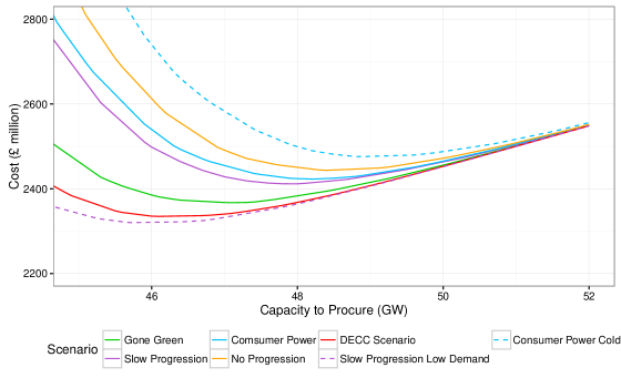
Figure 2: Combined cost of energy unserved and procured capacity, i.e. the cost functions $f_{i}(x)$, against capacity to procure $x$ for each of the five major scenarios and two variant “sensitivities” illustrated in Figure 14 of the 2015 ECR.

Figure 3 plots the regret functions $\hat{f}_{i}(x)$ against capacity to procure $x$ for the same seven scenarios illustrated in Figure 2. It is now seen that the two scenarios considered as “sensitivities”, plotted as dashed lines, and labelled Slow Progression Low Demand and Consumer Power Cold, are such that the relation (5) is satisfied with $k$ and $l$ indexing these two scenarios, and where the set $\mathcal{S}$ is here taken to be the set of seven scenarios illustrated. That this is so is unsurprising insofar as the seven regret functions $\hat{f}_{i}$, $i\in\mathcal{S}$, illustrated are clearly—to a good approximation—related to each other by argument shifts, as described in Section 2.3, and the two “sensitivities” identified above are clearly extreme in the sense discussed there.

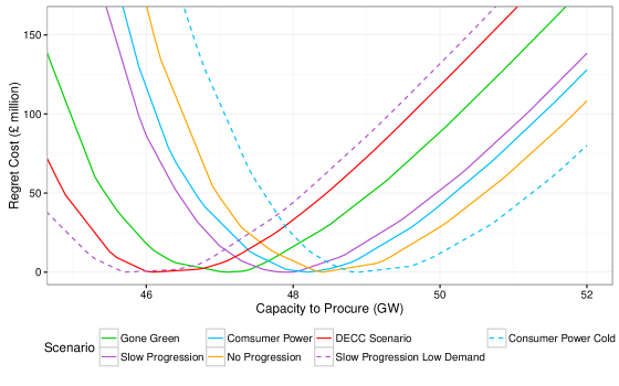
Figure 3: Regret functions $\hat{f}_{i}(x)$, against capacity to procure $x$ for each of the five major scenarios and two variant “sensitivities” illustrated in Figure 14 of the 2015 ECR.

We thus have $\hat{x}_{\mathcal{S}}=\hat{x}_{kl}=47.8$ GW—this value corresponding to the point of intersection of the regret functions for the above two “sensitivities”. All this continues to be the case when the set $\mathcal{S}$ is taken to consist of all 19 scenarios considered by the 2015 ECR; that the relation (5) then continues to hold with $k$ and $l$ indexing the same two “sensitivities” identified above (i.e. Slow Progression Low Demand and Consumer Power Cold) would be immediately apparent if, for example, all the 19 regret functions $\hat{f}_{i}$, $i\in\mathcal{S}$, were similarly plotted. Thus, for these 19 scenarios, the LWR capacity to procure is $47.8$ GW. Because the analysis of the 2015 ECR restricts the decision set $\mathcal{D}$ as described earlier, the capacity to procure recommended by that report is $47.9$ GW. This is the capacity to procure which precisely meets the reliability standard for one of the other (more minor) “sensitivities” considered in the report. However, a difference of $0.1$ GW is quite negligible in relation the possible impact of many of the other uncertainties involved, for example the true values of all the data underlying the analysis, or the values of the parameters $\mathrm{VOLL}$ and $\mathrm{CONE}$.

The lesson to be learned from the above analysis is that it is the two “extreme” scenarios or “sensitivities”, as identified above, which largely determine the LWR solution $\hat{x}_{\mathcal{S}}$. This solution is indifferent to the remaining scenarios so long as they do not themselves become more extreme than either of the above two. However, the “extreme” scenarios are often, as here, relatively minor ones. Considerable care nevertheless needs to be taken in their definition, precisely because it is they that are critical in determining the result of the analysis.

Alternative probabilistic analysis.

In line with the alternative, Bayesian, approach outlined in Section 2.4, we consider briefly what assignment of probabilities to scenarios would, on minimisation of the expression given by (11) so as to determine the solution $x_{\mathrm{bayes}}$ of a Bayesian analysis, result in the same value of the capacity to procure as that given by the solution $\hat{x}_{\mathcal{S}}$ of the LWR analysis. Since the cost functions $f_{i}$ may here reasonably be treated as differentiable, in addition to being convex, it follows from (11) that the sets of such probabilities $p_{i}$, $i\in\mathcal{S}$, are given by the solution of

$$\sum_{i\in\mathcal{S}}p_{i}f^{\prime}_{i}(\hat{x}_{\mathcal{S}})=0.$$ (23)

If the set $\mathcal{S}$ is taken to consist of all 19 scenarios of the 2015 ECR, then the sets of probabilities such that (23) holds form a 17-dimensional region. If we restrict attention to the two “extreme” sensitivities Slow Progression Low Demand and Consumer Power Cold which determine the LWR solution $\hat{x}_{\mathcal{S}}$ in the sense we have discussed in this paper, then some numerical experimentation shows that the assignment of a probability $0.68$ to the first of these and $0.32$ to the second (with a probability $0$ assigned to all the remaining scenarios) gives $x_{\mathrm{bayes}}=\hat{x}_{\mathcal{S}}=47.8$ GW as required. That these probabilities are approximately correct may also be seen (using (23)) from Figure 3.

A uniform assignment of probabilities $0.2$ to each of the five major scenarios considered by the 2015 ECR, and whose cost and regret functions are plotted in Figures 2 and 3, results in a capacity to procure of $x_{\mathrm{bayes}}=47.7$ GW. The exclusion of the DECC scenario (which, as previously explained, was not included in the final analysis of the report) increases this to $x_{\mathrm{bayes}}=48.0$ GW. A uniform assignment of probabilities to all 19 scenarios and “sensitivities” considered in the report again results in a value $x_{\mathrm{bayes}}=48.0$ GW (and $48.1$ GW if the DECC scenario is excluded). As it happens, none of these figures is here significantly different from the result of the LWR analysis. The latter is therefore reasonably robust, in this particular case, across a range of plausible assignments of probabilities to scenarios. That this is so is essentially a combination of the fact that the regret functions are close to being obtained from each other by simple shifts of their arguments as described in Section 2.3 and of the fact that the scenarios are relatively evenly spaced between their extremes.

5 Conclusion

Minimax and LWR analysis are commonly used for decision making whenever it is difficult, or perhaps inappropriate, to attach probabilities to possible future scenarios. We have shown that, for each of these two approaches and subject only to the convexity of the cost functions involved, it is always the case that there exist two “extreme” scenarios whose costs determine the outcome of the analysis in the sense we have made precise in Section 2. (The “extreme” scenarios need not be the same for each of the two approaches.) The results of either analysis are therefore particularly sensitive to the cost functions associated with the corresponding two “extreme” scenarios (while being largely unaffected by those associated with the remainder). In effect the results are sensitive to the definitions of these two scenarios, and indeed to whether or not they are even included in the specification of the problem. Great care is therefore required in applications to identify these scenarios and to consider their reasonableness.

We have also considered the common situation in which, at least to a good approximation, the regret functions differ from each other essentially by shifts of their arguments. In this case the two “extreme” scenarios are the obvious ones, namely those whose regret functions have the greatest relative shift in their arguments. It is further possible here to specify those sets of probabilities which, if assigned to scenarios under an alternative Bayesian analysis, would produce the answers as given by a LWR analysis in particular. At a minimum this assists in assessing the reasonableness of scenarios for inclusion in a LWR analysis.

A particular example of the above situation may occur in the case of determining a appropriate level of investment in order to control a risk. Here the cost functions associated with possible future scenarios are often the sum of an exponentially decaying and a linearly increasing component, and further the exponential decay rates are often approximately the same for all scenarios. This in the case with the problem of determining an appropriate level of electricity capacity procurement in Great Britain, where decisions must be made several years in advance, in spite of considerable uncertainty as to which of a number of future scenarios may occur, and where LWR analysis is currently used as the basis of decision making. We have considered in detail the analysis of the 2015 Electricity Capacity Report submitted to the UK Government by National Grid plc. Here the “extreme” scenarios determining the result of the LWR analysis are readily identified. Given these, the outcome of the LWR analysis appears reasonably robust against a variety of assignments of probabilities to the set of all the scenarios used.

References

- [1] J.O. Berger (1985). Statistical Decision Theory and Bayesian Analysis, 2nd edition. Springer, New York.
- [2] L.J. Savage (1951). The Theory of Statistical Decision. Journal of the American Statistical Association, 46 (253), 55–67.
- [3] G. Loomes and R. Sugden (1982). Regret theory: An alternative theory of rational choice under uncertainty. Economic Journal, 92 (4), 805–824.
- [4] D.E. Bell (1982). Regret in decision making under uncertainty. Operations Research, 30 (5), 961–981.
- [5] P.C. Fishburn (1982). The foundations of expected utility. Theory & Decision Library Springer, Netherlands.
- [6] National Grid (2015). EMR Electricity Capacity Report. June 2015.
- [7] Department of Energy and Climate Change (2013). EMR Consultation Annex C: Reliability Standard Methodology. July 2013.