SPECTRWM: Spectral Random Walk Method for the
Numerical Solution of Stochastic Partial Differential Equations

Abstract

The numerical solution of stochastic partial differential equations (SPDE) presents challenges not encountered in the simulation of PDEs or SDEs. Indeed, the roughness of the noise in conjunction with nonlinearities in the drift typically make these equations particularly stiff. In practice, this means that it is tricky to construct, operate, and validate numerical methods for SPDEs. This is especially true if one is interested in path-dependent expected values, long-time simulations, or in the simulation of SPDEs whose solutions have constraints on their domains. To address these numerical issues, this paper introduces a Markov jump process approximation for SPDEs, which we refer to as the spectral random walk method (SPECTRWM). The accuracy and ergodicity of SPECTRWM are verified in the context of a heat and overdamped Langevin SPDE, respectively. We also apply the method to Burgers and KPZ SPDEs.

I Introduction

Stochastic partial differential equations (SPDEs) describe the evolution of continuum systems with random fluctuations Walsh (1986); Hairer (2009); Da Prato and Zabczyk (2014). They are used as models for turbulence E et al. (1997); E and Vanden-Eijnden (2000); E et al. (2003); Mikulevicius and Rozovskii (2004); Da Prato and Debussche (2003); Hairer and Mattingly (2006), phase-field dynamics Funaki (1995); Kohn et al. (2007); Weber (2010), surface growth Kardar et al. (1986); Quastel (2011); Corwin (2012); Hairer (2013), neuronal activity Walsh (1986); Tuckwell (2005); Laing and Lord (2010), population dynamics/genetics Feller (1951); Dawson (1972); Fleming (1975) and interest rate fluctuations Cont (2005); Carmona and Tehranchi (2007). They also directly arise as space-time diffusion approximations of a large class of discrete models Kardar et al. (1986); Quastel (2011); Corwin (2012); Dembo and Tsai (2015). In addition to their use as mathematical models, their dynamic and ergodic properties are also leveraged to accelerate convergence of MCMC methods for sampling conditioned diffusions Stuart et al. (2004); Reznikoff and Vanden-Eijnden (2005); Hairer et al. (2005, 2007); Apte et al. (2007); Beskos et al. (2008). The importance of these equations lies in the basic fact that space-time Gaussian white noise is perhaps the simplest model of space-time random fluctuations. In this sense, the study of SPDEs is a quest to answer fundamental questions about continuum descriptions of high-dimensional discrete systems.

With few exceptions Hou et al. (2006); Luo (2006), current numerical methods for SPDEs are rooted in ideas from numerical PDE and SDE theory: replace the SPDE with a system of approximating SDEs by means of a finite difference or variational method, and then discretize these approximating SDEs in time using, e.g., a $\theta$-method like Euler-Maruyama or Crank Nicolson; see, e.g., Gyöngy and Nualart (1995, 1997); Davie and Gaines (2001); Walsh (2005); Alabert and Gyongy (2006); Jentzen and Kloeden (2009); Blomker and Jentzen (2013); Kruse (2014). However, there are particular problems associated with approximating SPDEs that motivate treating them differently. Here is a partial list.

• Stiffness. Due to the lack of regularity of the SPDE solution, the optimal time discretization error associated with spatio-temporal approximations is of strong order $1/4$ and weak order $1/2$ Davie and Gaines (2001); Walsh (2005). (To obtain these rates, one must assume that the spatial step size relates to the time step size via a CFL-type condition.) These rates contrast with the faster order of $2$ typically attainable for spatio-temporal approximations of the underlying PDE, and of strong order $1/2$ and weak order of $1$ typically attainable for SDEs using the Euler-Maruyama method Kloeden and E. (1995); Talay (1995); Milstein and Tretyakov (2004).

• Spurious Drift Terms. Hairer et al. showed that seemingly reasonable spatial discretizations of Burgers-like SPDEs do not converge to the right solution – even in a weak sense Hairer and Voss (2011); Hairer and Maas (2012); Hairer et al. (2014). Instead these discretizations converge to a (non-ergodic) SPDE with a spurious drift term that is a spatial analog of the Itô-Stratonovich correction. This numerical artifact is due to the spatial roughness of the SPDE solution. We refer the reader to Hairer and Voss (2011) for numerical results and an explanation of this numerical artifact, and to Hairer and Maas (2012); Hairer et al. (2014) for detailed proofs.

• Long-Time Simulation. Another problem is related to long-time simulation of ergodic SPDEs Prato and Zabczyk (1996); Cerrai (2001); Voss (2011). The aim of this type of simulation is to sample from the stationary distribution of the SPDE, and also to compute long-time dynamics. As far as we can tell, methods for ergodic SPDEs are currently limited to schemes that efficiently sample from the stationary distribution of Langevin SPDEs without too much concern about accurately representing their dynamics Beskos et al. (2008). The idea for this scheme comes from MCMC and numerical SDE theory Roberts and Tweedie (1996a, b); Bou-Rabee and Vanden-Eijnden (2010, 2012); Bou-Rabee and Hairer (2013); Bou-Rabee et al. (2014); Bou-Rabee (2014); Fathi (2014); Fathi et al. (2015), and basically involves combining a $\theta$-method for the approximating SDE with a Metropolis accept-reject step, which corrects the bias introduced by time discretization error. However, the results in Ref. Beskos et al. (2008) demonstrate that unless one chooses $\theta=1/2$ (a Crank-Nicholson discretization), the acceptance rate of the Metropolized $\theta$-scheme deteriorates in the space-time diffusion limit.

• Reflecting Solutions. Reflected SPDEs are an infinite-dimensional analog of SDEs with reflection Karatzas and Shreve (1991); Nualart and Pardoux (1992); Kushner and Dupuis (2001). They arise in the study of continuum models with constraints on the domain of their solutions, e.g., the Allen-Cahn SPDE with reflection at $\pm 1$ or positivity constraints in population or interest rate models Nualart and Pardoux (1992); Funaki and Olla (2001); Debussche and Zambotti (2007); Debussche and Goudenège (2011). In this context spatio-temporal methods may produce approximations that are outside the domain of definition of the SPDE.

In light of these practical problems, it is quite natural to approximate SPDEs using an algorithm that is more precisely tailored to the structure of their solutions. In this note we propose a simple way to do this. The idea is to approximate SPDEs by a Markov jump process that we refer to as the spectral random walk method (SPECTRWM). The departure point for constructing this approximation is a stable and accurate system of approximating SDEs, which may be obtained by, e.g., finite difference or spectral Galerkin methods Gyöngy and Nualart (1995, 1997); Walsh (2005). To be clear, we do not propose to solve the above problem regarding spurious drift terms, though we do confirm that incorrect discretizations lead to non-ergodic approximations to the Burgers and KPZ SPDEs. Given these approximating SDEs, we then proceed as follows: instead of discretizing these approximating SDEs in time – as is normally done – we discretize their infinitesimal generator in space Bou-Rabee and Vanden-Eijnden (2016). As we detail in §II below, an important ingredient in this construction is a basis given by the leading $n$ eigenfunctions associated to the linear part of the drift of the SPDE.

A realization of this Markov jump process approximation may be produced by iteratively computing its jumps and holding times: the jumps are taken in the direction of these eigenfunctions, while the holding time in any given state is an exponentially distributed random variable whose mean is a deterministic function of the SPDE coefficients evaluated at this state. In addition to being simple, the method allows several benefits:

• the jump size of the approximation is a parameter of the method;

• the time step size automatically adapts according to the stiffness of the SPDE coefficients;

• path-dependent expected values over slices of the SPDE solution in time can be approximated without incurring any time discretization error;

• every jump induces a global move in state space;

• they are multi-scale, in the sense that its jump size can be adapted to the different spatial scales of the SPDE problem; and,

• it can handle boundary conditions in reflected SPDEs in a natural way.

The SPECTRWM method and its properties are described in §II. Afterwards we test SPECTRWM on heat, overdamped Langevin, Burgers, and KPZ SPDEs, all with periodic boundary conditions.

Let us finish this introduction by remarking that SPECTRWM is a generalization of the Markov Chain Approximation Method (MCAM) to SPDEs. By now, MCAM is a well-established technique for the numerical solution of SDEs Kushner and Dupuis (2001); Bou-Rabee and Vanden-Eijnden (2016). The method was invented by Harold Kushner in the 1970s to approximate optimally controlled diffusion processes Kushner (1970); Kushner and Yu (1973, 1975); Kushner (1976a, b, 1977, 2001); Kushner and Dupuis (2001); Kushner (2002, 2004, 2006, 2011). However, because of their interest in stochastic control problems, these works focus on numerical solutions with gridded state spaces that admit a global matrix representation. In the statistical physics literature, this matrix representation was avoided and a Monte-Carlo method was used to simulate the numerical solution Elston and Doering (1996); Wang et al. (2003); Metzer (1999); Metzner et al. (2009); Latorre et al. (2011), and to be specific, this idea seems to go back to at least Elston and Doering (1996). Among these papers, the most general and geometrically flexible MCAM were the finite volume methods developed for over-damped Langevin equations presented in Latorre et al. (2011). More recently, the MCAM framework has been generalized to lessen the requirements on the underlying diffusion process Bou-Rabee and Vanden-Eijnden (2016). In particular, this generalization no longer requires that the domain of the diffusion process is bounded, that the infinitesimal generator of the diffusion process is symmetric or that the infinitesimal covariance of the diffusion process is diagonally dominant. This generalization is made possible by letting the state space of the numerical solution be gridless and by using Monte-Carlo methods to simulate the numerical solution, but at the same time, keeping the restriction that the jump size of the approximation is uniformly bounded. As we will see below, this property is essential to the stability and accuracy of SPECTRWM.

II Algorithm

We present two versions of SPECTRWM. The point of the first version is to illustrate basic concepts, and as such, it uses a spatial finite difference approximation of an SPDE on an evenly spaced grid in 1D. (This ‘academic’ version was used by the author in his mini-course entitled “Spectral Random Walk Method for the Numerical Solution of Stochastic Partial Differential Equations” at the 2016 Gene Golub SIAM Summer School.) The second version is based on a spectral Galerkin approximation, which, as we will see, is more general and more efficient than the academic one. Unless otherwise stated, we will mainly provide numerical verification of the academic version of SPECTRWM.

II.1 Academic Version

We present this version of SPECTRWM in the specific context of a one-dimensional SPDE with additive, space-time Gaussian white noise and a scalar noise coefficient. We assume that we are given a stable and accurate semi-discrete system that consists of a 1D grid with $n$ grid points, an initial condition on this grid, a spatial step size parameter $\Delta x>0$, and a system of approximating SDEs on $\mathbb{R}^{n}$ of the form:

$$du^{n}=\left[L_{n}u^{n}+F_{n}(u^{n})\right]dt+\sigma\sqrt{\frac{1}{\Delta x}}dW_{n}$$ (1)

where $L_{n}$ is an $n\times n$ discretization matrix associated to the linear part of the drift, $F_{n}$ is a discretization of the nonlinear part of the drift, $\sigma>0$ is a scalar constant, and $W_{n}$ is an $n$-dimensional Brownian motion. We assume that $L_{n}$ has an orthonormal set of $n$ eigenvectors $\{e_{i}\}$ with eigenvalues $\{\mu_{i}\}$. Implicit in this setup are the boundary conditions of the SPDE, which are typically built into (1). A typical example of $L_{n}$ is the discrete Laplacian for the standard finite difference method with periodic, Dirichlet, Neumann or mixed boundary conditions. In what follows, $u^{h}(t)\in\mathbb{R}^{n}$ denotes the Markov jump process approximation produced by SPECTRWM.

Algorithm II.1 (SPECTRWM: Academic Version).

Given the current time $t\geq 0$, the current state of the process $u_{h}(t)=v\in\mathbb{R}^{n}$, a spatial step size $\Delta x>0$, and a jump size $h>0$, the algorithm outputs an updated state $u_{h}(t+\delta t)$ at time $t+\delta t$ in three sub-steps.

(Step 1)

compute forward/backward jump rates:

$$J^{\pm}_{i}(v)=\frac{\sigma^{2}}{2h^{2}\Delta x}\exp\left(\pm\left(\mu_{i}v^{T}e_{i}+F_{n}(v)^{T}e_{i}\right)\frac{h\Delta x}{\sigma^{2}}\right)$$ (2)

for $1\leq i\leq n$.

(Step 2)

update time via

$$t_{1}=t_{0}+\delta t$$

where $\delta t$ is an exponentially distributed random variable with parameter

$$J(v)=\sum_{i=1}^{n}(J_{i}^{+}(v)+J_{i}^{-}(v))\;.$$ (3)

(Step 3)

update the state of the system by assuming that the process jumps forward/backward along the eigenvector $e_{i}$ to state $v\pm he_{i}$ with probability:

$$\Pr(u_{h}(t+\delta t)=v\pm he_{i}\mid u_{h}(t)=v)=\frac{J_{i}^{\pm}(v)}{J(v)}$$

for $1\leq i\leq n$.

We stress that this method is very simple and straightforward to implement. Note from (Step 3) that the algorithm moves by jumps in the semi-discrete space $\mathbb{R}^{n}$ in the directions of the eigenvectors of $L$. Moreover, the jump size is $h$, and these jumps alter every component, i.e., each jump induces a global system update. The time elapsed in each state $\delta t$ is an exponentially distributed random variable with parameter $J(v)$ given in (8), which is defined as the sum of the forward/backward jump rates from (Step 1). Also, the update rules in (Step 1) and (Step 2) only depend on the current state. Thus, the resulting process is a Markov jump process Revuz and Yor (1999); Protter (2004); Ethier and Kurtz (2009); Klebaner (2012).

This process has an infinitesimal generator that is given by:

$$Qf(v)=\sum_{1\leq i\leq n}J_{i}^{+}(v)\left(f(v+he_{i})-f(v)\right)+J_{i}^{-}(v)\left(f(v-he_{i})-f(v)\right)\;.$$ (4)

Using a Taylor expansion of $Qf(v)$ about $h=0$, in Appendix A we show that:

$$Qf(v)=v^{T}L_{n}\nabla f(v)+F_{n}(v)^{T}\nabla f(v)+\frac{\sigma^{2}}{2\Delta x}\operatorname{trace}(D^{2}f(v))+O(h^{2}\Delta x+h^{2})\;.$$ (5)

We recognize the leading order term in this expansion as the infinitesimal generator of the approximating SDE in (1). Thus, by choosing $h$ sufficiently small we can get arbitrarily close (in law) to the solution of the approximating SDE.

However, a very practical question remains: what is the computational cost of SPECTRWM? To address this question, we consider the scaling of SPECTRWM as the jump size decreases $h\to 0$; and, as the spatial step size decreases $\Delta x\to 0$ (or equivalently $n\to\infty$). In order to produce a single trajectory over $[0,t]$, the computational cost of SPECTRWM is proportional to the (random) number of steps $N(t)$ it takes for the approximation to reach $t$. In §4.3 of Bou-Rabee and Vanden-Eijnden (2016), it is shown that the mean of $N(t)$ is inversely proportional to the mean holding time. Thus, the mean holding time dictates the average cost of the algorithm, which from (Step 2) of Algorithm II.2 scales like $O(h^{2}/n^{2})$. This scaling of the mean holding time reflects the roughness of the noise and the fact that SPECTRWM is able to jump in the direction of any of the $n$ eigenmodes of $L$. However, it turns out we can do much better than this, by using a spectral Galerkin approximation, as we describe next.

II.2 Fast Version

Consider an SPDE with solution $u$ defined on a Hilbert space $H$ with inner product $\langle\cdot,\cdot\rangle$. Assume that the noise in the SPDE is additive space-time Gaussian white noise with scalar noise coefficient $\sigma>0$. Turning to the drift of the SPDE, assume this drift has a linear part of the form $Lu$ where $L$ is a linear operator with a complete orthonormal set of eigenfunctions $\{e_{i}\}$ and eigenvalues $\{\mu_{i}\}$ ordered such that $\mu_{i}\geq\mu_{i+1}$ for all natural numbers $i>0$. Typically $L$ is a uniformly elliptic differential operator with non-positive eigenvalues. In terms of these eigenfunctions, we define the finite-dimensional subspace $V_{n}=\operatorname{span}\{e_{1},\cdots,e_{n}\}$, which is the span of the eigenfunctions associated to the $n$ largest eigenvalues of $L$, and let $u^{n}$ denote the orthogonal projection of $u$ onto this finite-dimensional subspace $V_{n}$:

$$u^{n}=\sum_{i=1}^{n}\hat{u}_{i}^{n}e_{i}\;.$$

where we introduced the $n$ spectral coefficients: $\{\hat{u}_{i}^{n}=\langle u^{n},e_{i}\rangle~{}\mid~{}1\leq i\leq n\}$. The function $u^{n}$ is a standard spectral Galerkin approximation of $u$. Next we derive an $n$-dimensional system of approximating SDEs that the spectral coefficients of $u^{n}$ satisfy.

For this purpose, we approximate the space-time Wiener process in the SPDE by a truncated sum: $\sum_{i=1}^{n}B_{i}(t)e_{i}$ where $\{B_{i}\}$ are iid Brownian motions. Finally, let $\{\hat{F}_{i}\}$ denote the spectral coefficients of the rest of the drift of the SPDE in the finite-dimensional basis $\{e_{i}\}_{1\leq i\leq n}$. With these truncations in hand, the spectral coefficients of $u^{n}$ satisfy the following system of SDEs:

$$d\hat{u}_{i}^{n}=\left[\mu_{i}\hat{u}_{i}^{n}dt+\hat{F}_{i}(u^{n})\right]dt+\sigma dB_{i}$$ (6)

where $i$ ranges from $1$ to $n$. The fast version of SPECTRWM directly approximates these SDEs in the spectral domain. Let $u^{h}(t)$ denote the numerical solution produced by SPECTRWM.

Algorithm II.2 (SPECTRWM: Fast Version).

Given a jump size $h>0$, the current time $t\geq 0$, and the current state of the process $u^{h}(t)=v$, the algorithm outputs an updated state $u^{h}(t+\delta t)$ at time $t+\delta t$ in three sub-steps.

(Step 1)

compute forward/backward jump rates:

$$J^{\pm}_{i}(v)=\frac{\sigma^{2}}{2h^{2}}\exp\left(\pm\left(\mu_{i}\hat{v}_{i}+\hat{F}_{i}(v)\right)\frac{h}{\sigma^{2}}\right)$$ (7)

for $1\leq i\leq n$.

(Step 2)

update time via

$$t_{1}=t_{0}+\delta t$$

where $\delta t$ is an exponentially distributed random variable with parameter

$$J(v)=\sum_{i=1}^{n}\left[J_{i}^{+}(v)+J_{i}^{-}(v)\right]\;.$$ (8)

(Step 3)

update the state of the system by assuming that the process jumps forward/backward along the eigenvector $e_{i}$ with probability:

$$\Pr(u^{h}(t+\delta t)=v\pm he_{i}\mid u^{h}(t)=v)=\frac{J_{i}^{\pm}(v)}{J(v)}$$

for $1\leq i\leq n$.

Note that this version of SPECTRWM makes jumps of size $h$ in the individual spectral coefficients of $u^{h}$. Every jump in the spectral domain leads to a jump of size $h$ in $u^{h}$ along the corresponding eigenfunction. The generator of this version of SPECTRWM is identical in form to the generator given in (4) with forward/backward jump rates given in (7). However, in this case, the jumps and state of the system are in the spectral domain where the approximating SDEs are defined. In this case, a straightforward Taylor expansion, shows that the infinitesimal generator of this version is an $O(h^{2})$ approximation to the infinitesimal generator associated to the approximating SDEs in (6). This version of SPECTRWM is ‘fast’ because the mean holding time in this approximation scales like $O(h^{2}/n)$, in contrast to the $O(h^{2}/n^{2})$ scaling of the academic version.

III Heat SPDE

To assess accuracy of SPECTRWM, consider the heat SPDE on $[0,2\pi]$ with periodic boundary conditions at $0$ and $1$:

$$\begin{dcases}du=\left(\dfrac{\partial^{2}u}{\partial x^{2}}-\lambda u\right)dt+\sigma dW&\forall x\in[0,2\pi],t\geq 0\\ u(t,0)=u(t,2\pi)&\forall t\geq 0\;,\\ u(0,x)=\frac{c_{0}}{\sqrt{2\pi}}+\frac{1}{\sqrt{\pi}}\sum_{k\geq 1}\left(c_{-k}\cos(kx)+c_{k}\sin(kx)\right)&\forall x\in[0,2\pi]\;.\end{dcases}$$ (9)

where $\lambda\geq 0$ and $\sigma>0$ are parameters; and $\{c_{k}\}$ are the Fourier coefficients of the initial conditions. By the usual Fourier series argument, the solution to these equations at any time $t>0$ is a Gaussian process with mean

$$\mathbb{E}u(t,x)=\frac{c_{0}}{\sqrt{2\pi}}e^{-\mu_{0}t}+\frac{1}{\sqrt{\pi}}\sum_{k\geq 1}e^{-\mu_{k}t}\left(c_{-k}\cos(kx)+c_{k}\sin(kx)\right)$$ (10)

and spatial covariance

$$\mathbb{E}\left\{(u(t,x)-\mathbb{E}u(t,x))(u(t,y)-\mathbb{E}u(t,y))\right\}=$$ (11)

$$\qquad\qquad\begin{dcases}\frac{\sigma^{2}}{2\pi}t+\frac{\sigma^{2}}{\pi}\sum_{k\geq 1}\frac{1-e^{-2k^{2}t}}{2k^{2}}\cos(k(x-y))&\text{if $\lambda=0$}\\ \frac{\sigma^{2}}{2\pi}\frac{1-e^{-2\mu_{0}t}}{2\mu_{0}}+\frac{\sigma^{2}}{\pi}\sum_{k\geq 1}\frac{1-e^{-2\mu_{k}t}}{2\mu_{k}}\cos(k(x-y))&\text{if $\lambda>0$}\end{dcases}$$

where for convenience we have introduced $\mu_{k}=k^{2}+\lambda$. We use a truncation of (10) and (11) as a benchmark solution to verify the efficiency of the method in approximating expected values involving (a) the solution at a fixed time and (b) the entire path of the solution.

Remark III.1.

The dynamics of the heat SPDE involves a ‘competition’ between the dissipative drift term and the space-time Gaussian white noise. When $\lambda=0$, the noise wins in the sense that the zeroth order mode of the Fourier series solution is a Brownian motion, and as a consequence, the SPDE has no stationary distribution. This is reflected in the secular term appearing in (11) in the case $\lambda=0$. However, for any $\lambda>0$, the zeroth order mode of the Fourier series solution is an OU process, and the heat SPDE has a stationary distribution.

Referring to Figure 1, we discretize $[0,2\pi]$ using an evenly-spaced grid:

$$\left\{x_{i}=i\Delta x\mid 0\leq i\leq n\right\}$$

with spatial step size $\Delta x=2\pi/n$. Let $f_{i}=f(x_{i})$. On this grid, we approximate the diffusive part of the drift in (14) by a finite-difference method:

$$\frac{\partial^{2}f}{\partial x^{2}}(x_{i})=\dfrac{f_{(i+1)\bmod n}-2f_{i}+f_{(i-1)\bmod n}}{\Delta x^{2}}+O(\Delta x^{2})$$

which is valid if $f$ has four derivatives. The resulting discretization matrix is the discrete Laplacian with periodic boundary conditions in 1D, and its eigenvalues and eigenvectors are analytically known. Samples paths generated by SPECTRWM are given in Figure 2 for two different values of $\lambda$. The finite time weak accuracy of the scheme is verified in the graphs labelled (a) in the legend of Figure 6. The accuracy of the method in approximating the time integral of this covariance over $[0,1]$ (a path-dependent expected value) is verified in the graph labelled (b) in the figure legend. Both of these graphs are in agreement with the local consistency estimate provided in (5). Figure 4 shows that SPECTRWM is able to accurately represent the decay of high frequency modes. This is expected since the algorithm is based on a random walk in the spectral coefficients.

Figure 1: Grid. This cartoon shows the grid used for all of the test problems in this paper. The black dots mark the interior grid points, and the white dots mark the boundary grid points. Due to the periodic boundary conditions, the approximating SDEs only need to be evolved on the $n$ grid points: $x_{0},\cdots,x_{n-1}$. Also, for any function $f:[0,2\pi]\to\mathbb{R}$, we use the shorthand notation $f_{i}=f(x_{i})$ for $0\leq i\leq n$.

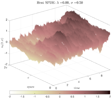
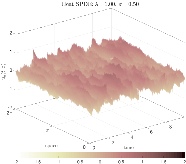
Figure 2: Heat SPDE on $[0,2\pi]$. Sample paths produced using SPECTRWM at the parameter values indicated in the figure title and with a trivial initial condition. Colors indicate the height of the surface, and are added in order to make the surface plots a bit more clear. These sample paths illustrate the stabilizing effect of the parameter $\lambda$.

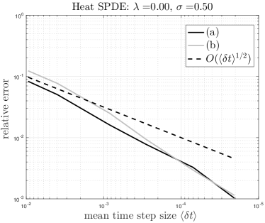
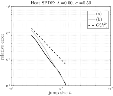
Figure 3: Heat SPDE on $[0,2\pi]$. This figure verifies the accuracy of SPECTRWM for the parameter values given in the figure title and for (a) the expected value of the solution squared at time $t=1$ and (b) the time integral of this expected value over $[0,1]$. The dashed lines are for reference.

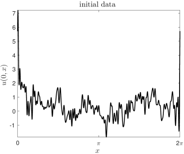
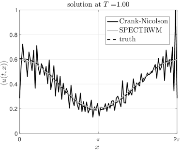
Figure 4: Heat SPDE on $[0,2\pi]$. This figure compares the fast version of SPECTRWM with $\sigma=1$, $\lambda=0$, and $n=11$ with the Crank-Nicolson scheme using $n=101$ grid points and $\Delta t=\Delta x$. The initial condition for this numerical test is shown in the left panel. The expected value of the true solution is the dashed line shown in the right panel. As is well known, the Crank-Nicolson scheme has trouble damping the high frequency modes, whereas the fast version of SPECTRWM does not have this issue.

IV Overdamped Langevin SPDE

To assess ergodicity of SPECTRWM, consider a nonlinear, overdamped Langevin SPDE:

$$\begin{dcases}du=\left(\dfrac{\partial^{2}u}{\partial x^{2}}-u^{3}\right)dt+\sigma dW&\forall x\in[0,2\pi],t\geq 0\\ u(t,0)=u(t,2\pi)&\forall t\geq 0\;,\\ \end{dcases}$$ (12)

with initial conditions that we will describe shortly. Using the same discretization as before, the approximating SDEs are themselves overdamped Langevin SDEs, which preserve a probability density function:

$$\pi^{n}(v)\propto\exp\left(-\Delta x\left(\sum_{0\leq i\leq n-1}\frac{v_{i}^{4}}{4}+\frac{v^{T}Lv}{2}\right)\right)$$

where $v=(v_{0},\cdots,v_{n-1})$. For the first test, we took an initial condition at very high energy as shown in Figure 5. This figure suggests that SPECTRWM is geometrically ergodic when the underlying SDE is. For the second test, we took a trivial initial condition, a very large jump size $h=\sqrt{\Delta x}$ and computed the accuracy of SPECTRWM. Following Chapter 2 of Bou-Rabee and Vanden-Eijnden (2016), we modified the jump rates so that the algorithm exactly preserves the stationary density of the approximating SDEs.

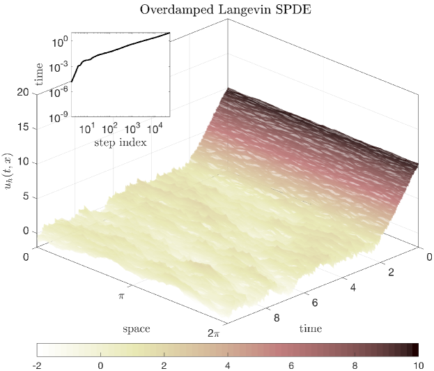
Figure 5: Overdamped Langevin SPDE on $[0,2\pi]$. Sample paths produced using SPECTRWM at the parameter values indicated in the figure title. Colors indicate the height of the surface, and are added in order to make the surface plots a bit more clear. These sample paths illustrate the stabilizing effect of the parameter $\lambda$.

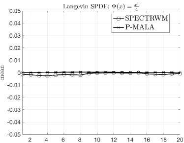
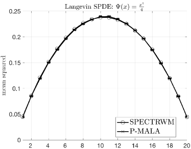
Figure 6: Overdamped Langevin SPDE on $[0,2\pi]$. This figure verifies the accuracy of SPECTRWM in computing the first and second moment of each component of the approximating SDE with $N=20$ grid points. The $x$-axis labels the components. We use as benchmark solution the preconditioned MALA algorithm, which obtains proposal moves from the $\theta$-method with $\theta=1/2$ Beskos et al. (2008).

V Burgers SPDE

We apply SPECTRWM to the following Burgers SPDE:

$$\begin{dcases}du=\left(\nu\dfrac{\partial^{2}u}{\partial x^{2}}-u\dfrac{\partial u}{\partial x}\right)dt+\sigma dW&\forall x\in[0,2\pi],t\geq 0\\ u(t,0)=u(t,2\pi)&\forall t\geq 0\;,\end{dcases}$$ (13)

with a bump function initial condition as depicted in Figure 7. To construct approximating SDEs, we use the same setup for the linear part and discretize the nonlinear advective term using either:

$$f\dfrac{\partial f}{\partial x}(x_{i})\approx\begin{dcases}\frac{1}{2\Delta x}\left(f^{2}_{(i+1)\bmod n}-f^{2}_{(i-1)\bmod n}\right)\\ \frac{1}{\Delta x}\left(f_{(i+1)\bmod n}-f_{i}\right)f_{i}\end{dcases}$$

As we confirm in Figure 7, the latter discretization leads to an approximation that is unstable. This qualitatively confirms the results in Hairer and Voss (2011); Hairer and Maas (2012). A quantitative comparison is not possible, because the precise form of the spurious drift term depends on the approximation being used.

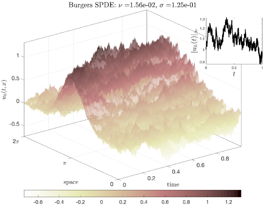
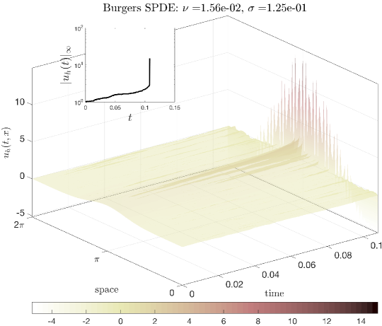
Figure 7: Burgers SPDE on $[0,2\pi]$. Sample paths produced using SPECTRWM at the parameter values indicated in the figure title. Colors indicate the height of the surface, and are added in order to make the surface plots a bit more clear. The left panel uses a valid semi-discrete approximation, while the right panel uses a semi-discrete approximation that converges to a non-ergodic SPDE.

VI KPZ SPDE

Here we apply SPECTRWM to the following KPZ SPDE:

$$\begin{dcases}du=\left(\dfrac{\partial^{2}u}{\partial x^{2}}+\lambda\left(\frac{\partial u}{\partial x}\right)^{2}\right)dt+\sigma dW&\forall x\in[0,2\pi],t\geq 0\\ u(t,0)=u(t,2\pi)&\forall t\geq 0\;,\end{dcases}$$ (14)

with a sinusoidal initial condition as depicted in Figure 8. To construct approximating SDEs, we use the previous setup for the linear part and discretize the nonlinear term using either:

$$\dfrac{\partial f}{\partial x}(x_{i})^{2}\approx\begin{dcases}\left(\frac{1}{2\Delta x}\left(f_{(i+1)\bmod n}-f_{(i-1)\bmod n}\right)\right)^{2}\\ \left(\frac{1}{\Delta x}\left(f_{(i+1)\bmod n}-f_{i}\right)\right)^{2}\end{dcases}$$

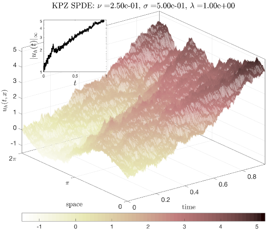
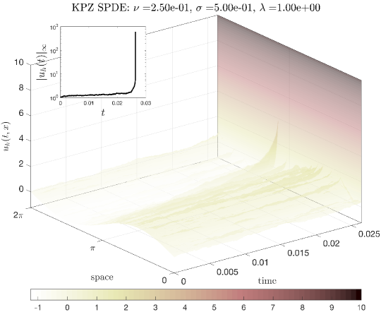
Figure 8: KPZ SPDE on $[0,2\pi]$. Sample paths produced using SPECTRWM at the parameter values indicated in the figure title. Colors indicate the height of the surface, and are added in order to make the surface plots a bit more clear. The left panel uses a valid semi-discrete approximation, while the right panel uses a semi-discrete approximation that converges to a non-ergodic SPDE.

VII Conclusion

What this paper has achieved is a generalization of the 1D random walk approximation of Brownian motion to SPDEs. Indeed, somewhat like the 1D random walk which makes jumps of fixed size $h$ to the left or right with equal probability, SPECTRWM jumps of fixed size $h$ forward or backward along the leading $n$ eigenfunctions of the linear part of the drift with jump rates that depend only on its current state. Moreover, just as the 1D random walk uses a mean holding time of $h^{2}$ for the sake of local accuracy, the mean holding time of SPECTRWM is also determined by local accuracy.

Aside from its mathematical interest, this generalization has practical uses. Indeed, since SPECTRWM is a (continuous-time) jump process with fixed jump size, this method solves in a natural way several problems that one encounters when simulating SPDEs, including their long-time simulation, the approximation of their path-dependent expected values, and by construction of its jumps, SPECTRWM is faithful to the domain of the SPDE solution. Being a Markov jump process, SPECTRWM also has the advantage of being easy to quantitatively analyze since it admits an infinitesimal generator, which can be used to analyze its stability and accuracy Bou-Rabee and Vanden-Eijnden (2016); Bou-Rabee and Sanz-Serna (2015).

Appendix A Local Consistency

Here we show that the infinitesimal generator of SPECTRWM is an accurate approximation of the infinitesimal generator of the approximating SDE given in (1). Referring to (4), Taylor expand the terms $f(v\pm he_{i})$ to obtain:

$$Qf(v)=\sum_{1\leq i\leq n} (J_{i}^{+}-J_{i}^{-})\left(h\nabla f(v)^{T}e_{i}+\frac{h^{3}}{6}D^{3}f(v)(e_{i},e_{i})+O(h^{5})\right)$$

$$+ (J_{i}^{+}+J_{i}^{-})\left(\frac{h^{2}}{2}D^{2}f(v)(e_{i},e_{i})+\frac{h^{4}}{12}D^{4}f(v)(e_{i},e_{i})+O(h^{6})\right)$$

To leading order, the forward/backward jump rates satisfy:

$$(J_{i}^{+}+J_{i}^{-}) =\frac{\sigma^{2}}{h^{2}\Delta x}+O(\Delta x)$$

$$(J_{i}^{+}-J_{i}^{-}) =\frac{1}{h}(\mu_{i}v^{T}e_{i}+F_{n}(v)^{T}e_{i})+O(h\Delta x^{2})$$

Thus,

$$Qf(v)=\sum_{1\leq i\leq n} (\mu_{i}v^{T}e_{i}+F_{n}(v)^{T}e_{i})\nabla f(v)^{T}e_{i}+\frac{\sigma^{2}}{2\Delta x}D^{2}f(v)(e_{i},e_{i})+O(h^{2}\Delta x+h^{2})$$

To finish, we use the fact that $e_{i}$ is an eigenvector of $L_{n}$ to obtain:

$$Qf(v) =\operatorname{trace}\left(\left(\nabla f(v)v^{T}L_{n}+\nabla f(v)F_{n}(v)^{T}+\frac{\sigma^{2}}{2\Delta x}D^{2}f(v)\right)\sum_{1\leq i\leq n}e_{i}e_{i}^{T}\right)+O(h^{2}\Delta x+h^{2})$$

$$=v^{T}L_{n}\nabla f(v)+F_{n}(v)^{T}\nabla f(v)+\frac{\sigma^{2}}{2\Delta x}\operatorname{trace}(D^{2}f(v))+O(h^{2}\Delta x+h^{2})$$

References

- Walsh (1986) J. B. Walsh, in École d’Été de Probabilités de Saint Flour XIV-1984 (Springer, 1986) pp. 265–439.
- Hairer (2009) M. Hairer, arXiv preprint arXiv:0907.4178 (2009).
- Da Prato and Zabczyk (2014) G. Da Prato and J. Zabczyk, Stochastic equations in infinite dimensions (Cambridge university press, 2014).
- E et al. (1997) W. E, K. Khanin, A. Mazel, and Y. Sinai, Physical review letters 78, 1904 (1997).
- E and Vanden-Eijnden (2000) W. E and E. Vanden-Eijnden, Commun. Pure Appl. Math 53, 852 (2000).
- E et al. (2003) W. E, K. Khanin, A. Mazel, and Y. Sinai, Ann Math 151, 877 (2003).
- Mikulevicius and Rozovskii (2004) R. Mikulevicius and B. L. Rozovskii, SIAM Journal on Mathematical Analysis 35, 1250 (2004).
- Da Prato and Debussche (2003) G. Da Prato and A. Debussche, Journal de mathématiques pures et appliquées 82, 877 (2003).
- Hairer and Mattingly (2006) M. Hairer and J. C. Mattingly, Annals of Mathematics , 993 (2006).
- Funaki (1995) T. Funaki, Probability Theory and Related Fields 102, 221 (1995).
- Kohn et al. (2007) R. V. Kohn, F. Otto, M. G. Reznikoff, and E. Vanden-Eijnden, Communications on pure and applied mathematics 60, 393 (2007).
- Weber (2010) H. Weber, Communications on Pure and Applied Mathematics 63, 1071 (2010).
- Kardar et al. (1986) M. Kardar, G. Parisi, and Y.-C. Zhang, Physical Review Letters 56, 889 (1986).
- Quastel (2011) J. Quastel, Current developments in mathematics 2011, 125 (2011).
- Corwin (2012) I. Corwin, Random matrices: Theory and applications 1, 1130001 (2012).
- Hairer (2013) M. Hairer, Annals of Mathematics 178, 559 (2013).
- Tuckwell (2005) H. C. Tuckwell, Introduction to theoretical neurobiology: volume 2, nonlinear and stochastic theories, Vol. 8 (Cambridge University Press, 2005).
- Laing and Lord (2010) C. Laing and G. J. Lord, Stochastic methods in neuroscience (Oxford University Press, 2010).
- Feller (1951) W. Feller, in Proceedings of the Second Berkeley Symposium on Mathematical Statistics and Probability (The Regents of the University of California, 1951).
- Dawson (1972) D. A. Dawson, Mathematical biosciences 15, 287 (1972).
- Fleming (1975) W. H. Fleming, Advances in Applied Probability 7, 100 (1975).
- Cont (2005) R. Cont, International Journal of theoretical and applied finance 8, 357 (2005).
- Carmona and Tehranchi (2007) R. Carmona and M. R. Tehranchi, Interest rate models: an infinite dimensional stochastic analysis perspective (Springer Science & Business Media, 2007).
- Dembo and Tsai (2015) A. Dembo and L.-C. Tsai, arXiv preprint arXiv:1503.03581 (2015).
- Stuart et al. (2004) A. M. Stuart, J. Voss, and P. Wilberg, Communications in Mathematical Sciences 2, 685 (2004).
- Reznikoff and Vanden-Eijnden (2005) M. G. Reznikoff and E. Vanden-Eijnden, Comptes Rendus Mathematique 340, 305 (2005).
- Hairer et al. (2005) M. Hairer, A. M. Stuart, J. Voss, and P. Wiberg, Communications in Mathematical Sciences 3, 587 (2005).
- Hairer et al. (2007) M. Hairer, A. M. Stuart, and J. Voss, The Annals of Applied Probability 17, 1657 (2007).
- Apte et al. (2007) A. Apte, M. Hairer, A. M. Stuart, and J. Voss, Physica D: Nonlinear Phenomena 230, 50 (2007).
- Beskos et al. (2008) A. Beskos, G. Roberts, A. Stuart, and J. Voss, Stochastics and Dynamics 8, 319 (2008).
- Hou et al. (2006) T. Y. Hou, W. Luo, B. Rozovskii, and H.-M. Zhou, Journal of Computational Physics 216, 687 (2006).
- Luo (2006) W. Luo, Wiener chaos expansion and numerical solutions of stochastic partial differential equations, Ph.D. thesis, California Institute of Technology (2006).
- Gyöngy and Nualart (1995) I. Gyöngy and D. Nualart, Stochastic Processes and their Applications 58, 57 (1995).
- Gyöngy and Nualart (1997) I. Gyöngy and D. Nualart, Potential Analysis 7, 725 (1997).
- Davie and Gaines (2001) A. Davie and J. Gaines, Mathematics of Computation 70, 121 (2001).
- Walsh (2005) J. B. Walsh, Potential Analysis 23, 1 (2005).
- Alabert and Gyongy (2006) A. Alabert and I. Gyongy, in From stochastic calculus to mathematical finance (Springer, 2006) pp. 1–15.
- Jentzen and Kloeden (2009) A. Jentzen and P. E. Kloeden, Milan Journal of Mathematics 77, 205 (2009).
- Blomker and Jentzen (2013) D. Blomker and A. Jentzen, SIAM Journal on Numerical Analysis 51, 694 (2013).
- Kruse (2014) R. Kruse, Stochastic Partial Differential Equations: Analysis and Computations 2, 471 (2014).
- Kloeden and E. (1995) P. E. Kloeden and P. E., Numerical Solution of Stochastic Differential Equations (Springer, Berlin, 1995).
- Talay (1995) D. Talay, in Probabilistic Methods in Applied Physics, Vol. 451, edited by P. Krèe and W. Wedig (Springer-Verlag, Berlin, 1995) pp. 54–96.
- Milstein and Tretyakov (2004) G. N. Milstein and M. V. Tretyakov, Stochastic Numerics for Mathematical Physics (Springer, Berlin, 2004).
- Hairer and Voss (2011) M. Hairer and J. Voss, Journal of Nonlinear Science 21, 897 (2011).
- Hairer and Maas (2012) M. Hairer and J. Maas, The Annals of Probability 40, 1675 (2012).
- Hairer et al. (2014) M. Hairer, J. Maas, and H. Weber, Communications on Pure and Applied Mathematics 67, 776 (2014).
- Prato and Zabczyk (1996) G. D. Prato and J. Zabczyk, Ergodicity for Infinite Dimensional Systems (Cambridge University Press, 1996).
- Cerrai (2001) S. Cerrai, Second order PDE’s in finite and infinite dimension: a probabilistic approach, Vol. 1762 (Springer, 2001).
- Voss (2011) J. Voss, arXiv preprint arXiv:1110.4653 (2011).
- Roberts and Tweedie (1996a) G. O. Roberts and R. L. Tweedie, Biometrika 1, 95 (1996a), http://biomet.oxfordjournals.org/content/83/1/95.abstract.
- Roberts and Tweedie (1996b) G. O. Roberts and R. L. Tweedie, Bernoulli 2, 341 (1996b), http://projecteuclid.org/euclid.bj/1178291835.
- Bou-Rabee and Vanden-Eijnden (2010) N. Bou-Rabee and E. Vanden-Eijnden, Comm Pure and Appl Math 63, 655 (2010), http://www.crab.rutgers.edu/~nb361/mypapers/BoVa2010.pdf.
- Bou-Rabee and Vanden-Eijnden (2012) N. Bou-Rabee and E. Vanden-Eijnden, J Comput Phys 231, 2565 (2012), http://www.crab.rutgers.edu/~nb361/mypapers/BoVa2012.pdf.
- Bou-Rabee and Hairer (2013) N. Bou-Rabee and M. Hairer, IMA J of Numer Anal 33, 80 (2013), http://www.crab.rutgers.edu/~nb361/mypapers/BoHa2013.pdf.
- Bou-Rabee et al. (2014) N. Bou-Rabee, A. Donev, and E. Vanden-Eijnden, Multiscale Modeling & Simulation 12, 781 (2014), http://www.crab.rutgers.edu/~nb361/mypapers/BoDoVa2014.pdf.
- Bou-Rabee (2014) N. Bou-Rabee, Entropy 16, 138 (2014), http://www.crab.rutgers.edu/~nb361/mypapers/Bo2014.pdf.
- Fathi (2014) M. Fathi, Theoretical and numerical study of a few stochastic models of statistical physics, Ph.D. thesis, Université Pierre et Marie Curie-Paris VI (2014).
- Fathi et al. (2015) M. Fathi, A.-A. Homman, and G. Stoltz, ESAIM: Proceedings and Surveys 48, 341 (2015).
- Karatzas and Shreve (1991) I. Karatzas and S. E. Shreve, Brownian motion and stochastic calculus, 2nd ed., Vol. 113 (Springer-Verlag, 1991).
- Nualart and Pardoux (1992) D. Nualart and E. Pardoux, Probability Theory and Related Fields 93, 77 (1992).
- Kushner and Dupuis (2001) H. J. Kushner and P. Dupuis, Numerical Methods for Stochastic Control Problems in Continuous Time (Springer, 2001).
- Funaki and Olla (2001) T. Funaki and S. Olla, Stochastic processes and their applications 94, 1 (2001).
- Debussche and Zambotti (2007) A. Debussche and L. Zambotti, The Annals of Probability 35, 1706 (2007).
- Debussche and Goudenège (2011) A. Debussche and L. Goudenège, SIAM Journal on Mathematical Analysis 43, 1473 (2011).
- Bou-Rabee and Vanden-Eijnden (2016) N. Bou-Rabee and E. Vanden-Eijnden, “Continuous-time random walks for the numerical solution of stochastic differential equations,” (2016), http://www.ams.org/cgi-bin/mstrack/accepted_papers/memo.
- Kushner (1970) H. J. Kushner, J Math Anal Appl 32, 77 (1970).
- Kushner and Yu (1973) H. J. Kushner and C.-F. Yu, J Math Anal Appl 43, 603 (1973).
- Kushner and Yu (1975) H. J. Kushner and C.-F. Yu, J Math Anal Appl 51, 359 (1975).
- Kushner (1976a) H. J. Kushner, J Math Anal Appl 53, 251 (1976a).
- Kushner (1976b) H. J. Kushner, J Math Anal Appl 53, 644 (1976b).
- Kushner (1977) H. J. Kushner, Probability methods for approximations in stochastic control and for elliptic equations (Academic Press, 1977).
- Kushner (2001) H. J. Kushner, Heavy traffic analysis of controlled queueing and communication networks, 1st ed., Vol. 47 (Springer Science & Business Media, 2001).
- Kushner (2002) H. J. Kushner, SIAM journal on control and optimization 41, 457 (2002).
- Kushner (2004) H. J. Kushner, SIAM journal on control and optimization 42, 1911 (2004).
- Kushner (2006) H. J. Kushner, Stochastics An International Journal of Probability and Stochastic Processes 78, 343 (2006).
- Kushner (2011) H. J. Kushner, Stochastics: An International Journal of Probability and Stochastic Processes 83, 277 (2011).
- Elston and Doering (1996) T. C. Elston and C. R. Doering, J Stat Phys 83, 359 (1996).
- Wang et al. (2003) H. Wang, C. S. Peskin, and T. C. Elston, Journal of theoretical biology 221, 491 (2003).
- Metzer (1999) P. Metzer, Transition Path Theory for Markov Processes, Doctoral thesis, Free University Berlin (1999).
- Metzner et al. (2009) P. Metzner, C. Schütte, and E. Vanden-Eijnden, Multiscale Modeling & Simulation 7, 1192 (2009).
- Latorre et al. (2011) J. C. Latorre, P. Metzner, C. Hartmann, and C. Schütte, Comm Math Sci 9, 1051 (2011).
- Revuz and Yor (1999) D. Revuz and M. Yor, Continuous martingales and Brownian motion, 3rd ed., Grundlehren der Mathematischen Wissenschaften [Fundamental Principles of Mathematical Sciences], Vol. 293 (Springer-Verlag, Berlin, 1999) pp. xiv+602.
- Protter (2004) P. E. Protter, Stochastic Integration and Differential Equations, Vol. 21 (Springer, 2004).
- Ethier and Kurtz (2009) S. N. Ethier and T. G. Kurtz, Markov processes: characterization and convergence, Vol. 282 (John Wiley & Sons, 2009).
- Klebaner (2012) F. C. Klebaner, Introduction to stochastic calculus with applications, Vol. 57 (Imperial College Press, 2012).
- Bou-Rabee and Sanz-Serna (2015) N. Bou-Rabee and J. M. Sanz-Serna, “Randomized Hamiltonian Monte Carlo,” (2015), arXiv:1511.09382 [math.PR].