Nonperturbative quasi-classical theory of the nonlinear electrodynamic response of graphene

Abstract

An electromagnetic response of a single graphene layer to a uniform, arbitrarily strong electric field ${\bm{E}}(t)$ is calculated by solving the kinetic Boltzmann equation within the relaxation-time approximation. The theory is valid at low (microwave, terahertz, infrared) frequencies satisfying the condition $\hbar\omega\lesssim 2E_{F}$, where $E_{F}$ is the Fermi energy. We investigate the saturable absorption and higher harmonics generation effects, as well as the transmission, reflection and absorption of radiation incident on the graphene layer, as a function of the frequency and power of the incident radiation and of the ratio of the radiative to scattering damping rates. We show that the optical bistability effect, predicted in Phys. Rev. B 90, 125425 (2014) on the basis of a perturbative approach, disappears when the problem is solved exactly. We show that, under the action of a high-power radiation ($\gtrsim 100$ kW/cm²) both the reflection and absorption coefficients strongly decrease and the layer becomes transparent.

I Introduction

One of the most distinctive features of graphene, important for its electronic and optoelectronic applications, is the linear energy dispersion ${\cal E}_{\pm}({\bm{p}})=\pm v_{F}|{\bm{p}}|$ of quasi-particles – electrons and holes – in this material Castro Neto et al. (2009). It was shown Mikhailov (2007), within the quasi-classical approach, that the linear energy dispersion of graphene electrons should lead to its strongly nonlinear electrodynamic response. Indeed, under the action of a time-dependent electric field proportional to $\cos\omega t$ the electron momentum should oscillate, according to the Newton’s equation of motion, as $\sin\omega t$. In conventional materials with the parabolic energy dispersion the velocity, and hence the current, are proportional to the momentum, therefore the current oscillates with the same frequency $\omega$. In contrast, in graphene the velocity ${\bm{v}}={\bm{\nabla}}_{\bm{p}}{\cal E}_{\pm}({\bm{p}})=v_{F}{\bm{p}}/|{\bm{p}}|$ is proportional not to the momentum but, roughly, to the sign of the momentum. As a result the time dependence of the current $j$ has a step-like form,

$$j\propto en_{s}v_{F}{\rm sgn}(\sin\omega t)=en_{s}v_{F}\frac{4}{\pi}\left(\sin\omega t)+\frac{1}{3}\sin(3\omega t)+\dots\right),$$ (1)

and contains higher frequency harmonics Mikhailov (2007) (here $n_{s}$ is the surface electron density in graphene).

Graphene is thus intrinsically a strongly nonlinear material, and all the variety of nonlinear phenomena – harmonics generation, frequency mixing, saturable absorption, and so on, – should be observed in graphene in relatively low electric fields. The prediction Mikhailov (2007) was experimentally confirmed in many papers where harmonics generation Dragoman et al. (2010); Bykov et al. (2012); Kumar et al. (2013); Hong et al. (2013); An et al. (2013, 2014); Lin et al. (2014), four-wave mixing Hendry et al. (2010); Hotopan et al. (2011); Gu et al. (2012), saturable absorption and Kerr effect Zhang et al. (2012); Popa et al. (2010, 2011); Vermeulen et al. (2016), plasmon related nonlinear phenomena Constant et al. (2016), and other effects Mics et al. (2015) were observed. This also stimulated further theoretical studies of different nonlinear electrodynamic effects in graphene Mikhailov and Ziegler (2008); Mikhailov (2009a, b); Dean and van Driel (2009, 2010); Ishikawa (2010); Mikhailov (2011); Jafari (2012); Mikhailov and Beba (2012); Avetissian et al. (2013); Mikhailov (2013); Cheng et al. (2014a, b); Yao et al. (2014); Smirnova et al. (2014); Peres et al. (2014); Cox and de Abajo (2014, 2015); Savostianova and Mikhailov (2015); Cheng et al. (2015); *Cheng16; Mikhailov (2016); Mikhailov et al. (2016); Rostami and Polini (2016); Cox et al. (2016); Marini et al. (2016); Sharif et al. (2016a, b); Cheng et al. (2016b); Wang et al. (2016); Tokman et al. (2016); Rostami et al. (2016), for recent reviews see Glazov and Ganichev (2014); Hartmann et al. (2014). Theoretically, analytical results for the nonlinear electromagnetic response of a uniform graphene layer were obtained both at low (microwave, terahertz, $\hbar\omega\lesssim 2E_{F}$, Refs. Mikhailov (2007); Mikhailov and Ziegler (2008); Mikhailov (2011); Yao et al. (2014); Peres et al. (2014)), and high (infrared, optical, $\hbar\omega\gtrsim 2E_{F}$, Refs. Ishikawa (2010); Cheng et al. (2014a, b, 2015); *Cheng16; Mikhailov (2016); Rostami and Polini (2016); Marini et al. (2016); Wang et al. (2016); Cheng et al. (2016b); Tokman et al. (2016)), frequencies; here $E_{F}$ is the Fermi energy of graphene electrons (or holes) and $\omega$ is the typical radiation frequency. In the latter case the inter-band electronic transitions have to be taken into account and the problem requires a quantum-mechanical treatment. In the former case it is sufficient to consider only the intra-band transitions and the problem can be solved within the quasi-classical Boltzmann equation.

In most so far published theoretical papers the nonlinear electromagnetic response of graphene was studied within the perturbation theory. In this paper we study the low-frequency ($\hbar\omega\lesssim 2E_{F}$) electromagnetic response of graphene non-perturbatively. We solve the quasiclassical Boltzmann equation in the relaxation time ($\tau$) approximation,

$$\frac{\partial f(\bm{p},t)}{\partial t}+F_{x}(t)\frac{\partial f(\bm{p},t)}{\partial p_{x}}=-\frac{f(\bm{p},t)-f_{0}(\bm{p})}{\tau},$$ (2)

$F_{x}(t)=-eE_{x}(t)$, not assuming that the ac electric field $E_{x}(t)$ acting on graphene electrons is weak; here $f_{0}(\bm{p})$ is the equilibrium (Fermi-Dirac) distribution function. Having found the non-perturbative electron distribution function we then calculate the nonlinear current and analyze the saturable absorption, harmonic generation and some other nonlinear effects.

The $\tau$-approximation (2) that we use in this work offers a simple but efficient way to take into account the charge carrier scattering processes. It often allows one to get even analytical solutions of complicated nonlinear response problems (see Refs. Cheng et al. (2014b); Yao et al. (2014); Peres et al. (2014); Cheng et al. (2015); Mikhailov (2016); Mikhailov et al. (2016); Cheng et al. (2016b), as well as this work). The time $\tau$ in (2) is a phenomenological parameter which may depend on temperature, chemical potential and radiation power. The relaxation-time approximation may fail near resonances related to inter-band transitions, in particular, when a nonlinear response of intrinsic graphene ($E_{F}=0$) is considered Romanets and Vasko (2010, 2011). In the present work we focus on the quasi-classical frequency range $\hbar\omega\lesssim 2E_{F}$, where the inter-band transitions are not the case, which justifies the use of the approximation (2).

Among the nonlinear phenomena which turned out to be useful to study within the nonperturbative theory is the so called optical bistability. This effect was predicted in graphene at terahertz frequencies ($\hbar\omega\lesssim 2E_{F}$) in a recent work Peres et al. (2014). In that paper the authors considered the incidence of radiation (with the frequency $\omega$ and the intensity ${\cal J}_{i}$) on a graphene layer, and calculated the intensity of the transmitted wave at the same frequency ${\cal J}_{t}$. Solving the Boltzmann equation (2) they showed that, at certain (large) values of the parameter

$$\beta=\left(\frac{2\alpha E_{F}}{\hbar\omega}\right)^{2},$$ (3)

the dependence ${\cal J}_{t}({\cal J}_{i})$ has an $S$-shaped form, i.e., the function ${\cal J}_{t}({\cal J}_{i})$ is multivalued; here $\alpha=e^{2}/\hbar c$ is the fine structure constant. This result was derived in the collisionless approximation, $\omega\tau\gg 1$, and in low electric fields, meaning that the solution of the Boltzmann equation was expanded in powers of the parameter

$${\cal F}_{\omega}=\frac{eE_{0}}{\hbar\omega k_{F}},$$ (4)

taking the third ($\propto{\cal F}_{\omega}^{3}$) and fifth ($\propto{\cal F}_{\omega}^{5}$) order terms into account; here $E_{0}$ is the electric field amplitude and $k_{F}$ is the Fermi wave-vector.

The results of Ref. Peres et al. (2014) cause a few questions. First, the low-frequency response of graphene was investigated, in the collisionless approximation $\omega\tau\gg 1$, in Ref. Mikhailov (2007). In the paper Mikhailov (2007) the right-hand side of Eq. (2) was assumed to be zero from the outset, while in Ref. Peres et al. (2014) equation (2) was first solved with a finite right-hand side and after that the limit $\omega\tau\gg 1$ was taken. The results of Refs. Mikhailov (2007) and Peres et al. (2014) coincide for the third-order response (for the $3\omega$-Fourier component of the current), but differ (by a factor of three) for the $\omega$-Fourier component. The question why the two different methods give different results under the same condition $\omega\tau\gg 1$ remained unclear (a short comment on page 3 of Ref. Peres et al. (2014) does not actually explain this contradiction).

Second, the $S$-shaped ${\cal J}_{t}({\cal J}_{i})$–characteristics was obtained in Ref. Peres et al. (2014) by using the perturbative theory in the electric field parameter ${\cal F}_{\omega}$, which supposes, strictly speaking, that ${\cal F}_{\omega}$ should be small, ${\cal F}_{\omega}\ll 1$. But the characteristic point of the $S$-shaped ${\cal J}_{t}({\cal J}_{i})$–curve, in which the derivative $d{\cal J}_{t}/d{\cal J}_{i}$ becomes infinite, $d{\cal J}_{t}/d{\cal J}_{i}=\infty$, lie at ${\cal F}_{\omega}\simeq 1$, see Figure 3 in Ref. Peres et al. (2014). This causes some doubts in the validity of the prediction; the question, whether the predicted bistability survives if to solve the problem exactly, not expanding the result in powers of ${\cal F}_{\omega}$, remained unanswered.

The third question concerns the applicability area of the predicted effect. As seen from Figure 3 of Ref. Peres et al. (2014), the optical bistability takes place only if $\beta\gtrsim 2$. This means that the condition $\hbar\omega\lesssim\alpha E_{F}$ should be satisfied. On the other hand, $\omega\tau$ should be much larger than unity. This leaves a narrow window for the frequency, $\alpha E_{F}/\hbar\gtrsim\omega\gg 1/\tau$ and imposes rather strong restrictions on the Fermi energy, $E_{F}\gg 137\hbar/\tau$, and the mean free path $l=v_{F}\tau$, $k_{F}l\gg 137$. The question arises, whether and how the predicted effect is modified if to do not assume that $\omega\tau\gg 1$ and $k_{F}l\gg 137$.

In this paper we answer the three above formulated questions. We solve the problem exactly, not assuming that the frequency parameter $\omega\tau$ is large and the field parameter ${\cal F}_{\omega}$ is small. We show that, if to solve the problem exactly (non-perturbatively), the “optical bistability” effect disappears. The ${\cal J}_{t}({\cal J}_{i})$–characteristics of graphene remains a nonlinear but single-valued function which physically corresponds to the saturable absorption but not to the optical bistability. We also show that at small values of the frequency parameter $\omega\tau$ (the limit that was not considered in Ref. Peres et al. (2014)) the nonlinear features are in fact more pronounced than in the limit $\omega\tau\gg 1$.

The paper is organized as follows. In Section II we formulate the non-perturbative nonlinear response problem and solve it. In Section III we analyze the obtained results in several different cases including the Kerr and harmonics generation effects. In Section IV the results are summarized and conclusions are drawn. Some technical details are given in the Appendixes.

II Theory

II.1 Formulation of the problem

We consider a homogeneous two-dimensional (2D) electron gas under the action of a uniform electric field $E_{x}(t)$. The 2D layer occupies the plane $z=0$ and the spectrum of electrons in it, ${\cal E}({\bm{p}})\equiv{\cal E}(p_{x},p_{y})$, can be parabolic, like in a semiconducting GaAs quantum well, or linear, like in semimetallic graphene. Further, we consider an experimentally relevant situation, when the electric field $E_{x}(t)$ is zero at $t<0$ and is switched on at $t=0$ being, in general, an arbitrary function $\tilde{E}_{x}(t)$ at $t>0$, $E_{x}(t)=\theta(t)\tilde{E}_{x}(t)$. The distribution of electrons in the momentum space is described, respectively, by the Fermi-Dirac function

$$f_{0}({\bm{p}})\equiv f_{0}(p_{x},p_{y})=\left[1+\exp\left(\frac{{\cal E}({\bm{p}})-\mu}{T}\right)\right]^{-1},$$ (5)

at $t<0$ and by Boltzmann equation (2) at $t>0$; here $\mu$ is the chemical potential and $T$ is the temperature. The scattering of electrons is taken into account within the momentum relaxation time approximation, Eq. (2), where $\tau$ is assumed to be energy independent. Our task is to find the distribution function $f(\bm{p},t)\equiv f(p_{x},p_{y},t)$, which satisfies Boltzmann equation (2) at $t>0$ and the initial condition

$$f(p_{x},p_{y},t=0)=f_{0}(p_{x},p_{y})$$ (6)

at $t=0$, not imposing any restriction of the value of the scattering parameter $\omega\tau$ and not expanding the solution in powers of the electric field.

II.2 Solution of Boltzmann equation

The formulated problem is often solved by the method of characteristics, see, e.g., Ref. Peres et al. (2014). We use the Fourier technique which, in our opinion, is more transparent. First, we notice that the momentum component $p_{y}$ in Eq. (2) is a parameter, and the functions $f_{0}(p_{x},p_{y})$ and $f(p_{x},p_{y},t)$ tend to zero at $p_{x}\to\pm\infty$. Therefore we can expand these functions in Fourier integrals over $p_{x}$:

$$f(p_{x},p_{y},t)=\int_{-\infty}^{\infty}dse^{isp_{x}}\tilde{f}(s,p_{y},t),$$ (7)

$$f_{0}(p_{x},p_{y})=\int_{-\infty}^{\infty}dse^{isp_{x}}\tilde{f}_{0}(s,p_{y}).$$ (8)

Substituting these expansions in Boltzmann equation (2) we get an inhomogeneous ordinary differential equation for the function $\tilde{f}(s,p_{y},t)$

$$\frac{d\tilde{f}(s,p_{y},t)}{dt}+\left(isF(t)+\frac{1}{\tau}\right)\tilde{f}(s,p_{y},t)=\frac{\tilde{f}_{0}(s,p_{y})}{\tau},\ \ \ t>0,$$ (9)

with the initial condition

$$\tilde{f}(s,p_{y},t=0)=\tilde{f}_{0}(s,p_{y}).$$ (10)

($s$ and $p_{y}$ are parameters here). Eq. (9) can be solved by the separation of variables and the variation of constants techniques, which leads to the general solution

$$\tilde{f}(s,p_{y},t)=A_{0}e^{-\gamma t-is\int_{-\infty}^{t}F(t^{\prime})dt^{\prime}}+\gamma\tilde{f}_{0}(s,p_{y})\int_{-\infty}^{t}e^{-\gamma(t-t^{\prime})-is\int_{t^{\prime}}^{t}F(t^{\prime\prime})dt^{\prime\prime}}dt^{\prime},$$ (11)

where $\gamma=1/\tau$ and $A_{0}$ is the integration constant. At $t<0$ the force $F_{x}(t)$ equals zero, hence, the integrals $\int_{-\infty}^{t}F(t^{\prime})dt^{\prime}$ and $\int_{t^{\prime}}^{t}F(t^{\prime\prime})dt^{\prime\prime}$ vanish and we get

$$\tilde{f}(s,p_{y},t<0)=A_{0}e^{-\gamma t}+\tilde{f}_{0}(s,p_{y}).$$ (12)

Comparing (12) with (10) we see that $A_{0}=0$. Substituting now (11) into (7) we obtain, see Appendix A:

$$f(p_{x},p_{y},t)=\gamma\int_{-\infty}^{t}e^{-\gamma(t-t^{\prime})}f_{0}\left(p_{x}-\int_{t^{\prime}}^{t}F(t^{\prime\prime})dt^{\prime\prime},p_{y}\right)dt^{\prime}.$$ (13)

The function (13) satisfies Boltzmann equation (2) and the initial condition (6). At $t>0$ it can be rewritten as Ignatov and Romanov (1976) (Appendix A):

$$f(p_{x},p_{y},t)=e^{-\gamma t}f_{0}\left(p_{x}-\int_{0}^{t}\tilde{F}(t^{\prime\prime})dt^{\prime\prime},p_{y}\right)+\gamma\int_{0}^{t}e^{-\gamma(t-t^{\prime})}f_{0}\left(p_{x}-\int_{t^{\prime}}^{t}\tilde{F}(t^{\prime\prime})dt^{\prime\prime},p_{y}\right)dt^{\prime}.$$ (14)

The difference between the results of Refs. Mikhailov (2007) and Peres et al. (2014) can now be clarified. In Ref. Mikhailov (2007) the limit $\tau\to\infty$ was taken from the outset. Assuming $\gamma=1/\tau\to 0$ in (14) we get

$$\lim_{\gamma\to 0}f(p_{x},p_{y},t)=f_{0}\left(p_{x}-\int_{0}^{t}\tilde{F}(t^{\prime\prime})dt^{\prime\prime},p_{y}\right).$$ (15)

This result coincides with the one obtained in Ref. Mikhailov (2007) (if to assume that the force $\tilde{F}(t)$ contains only one frequency harmonic). One sees that the limit $\gamma\to 0$ ($\tau\to\infty$) actually means $\gamma t\ll 1$ or $t\ll\tau$, i.e., the result of Ref. Mikhailov (2007), Eq. (15), is valid under the conditions

$$\omega\tau\gg 1\textrm{ and }t\ll\tau\ \ \textrm{ in Ref. \cite[cite]{\@@bibref{Authors Phrase1YearPhrase2}{Mikhailov07e}{\@@citephrase{(}}{\@@citephrase{)}}}}.$$ (16)

In the opposite limit, $\gamma t\gg 1$, Eq. (14) gives

$$\lim_{\gamma t\to\infty}f(p_{x},p_{y},t)=\int^{\infty}_{0}e^{-\xi}f_{0}\left(p_{x}-\int_{t-\xi\tau}^{t}\tilde{F}(t^{\prime\prime})dt^{\prime\prime},p_{y}\right)d\xi,$$ (17)

see Appendix A. This result coincides with the one obtained in Ref. Peres et al. (2014) (if to assume that the force $\tilde{F}(t)$ contains only one frequency harmonic). It is thus valid at

$$\omega\tau\gg 1\textrm{ and }t\gg\tau\ \ \textrm{ in Ref. \cite[cite]{\@@bibref{Authors Phrase1YearPhrase2}{Peres14}{\@@citephrase{(}}{\@@citephrase{)}}}}.$$ (18)

Thus, being both obtained under the condition $\omega\tau\gg 1$, the results of Refs. Mikhailov (2007) and Peres et al. (2014) are valid in different time intervals, Eqs. (16) and (18), respectively. Below, we will only consider the steady-state solution (17), which is valid at $t\gg\tau$ and which we will simply call $f(p_{x},p_{y},t)$.

II.3 Response to a monochromatic excitation

If $\tilde{F}(t)$ is a periodic function with a period $T$, the distribution function $f(p_{x},p_{y},t)$, Eq. (17), is also periodic with the same period. Assume now that the external force is given by a monochromatic sine function,

$$\tilde{F}(t)=-eE_{0}\sin\omega t,$$ (19)

and calculate the induced electric current

$$j_{x}(t)=-\frac{e}{S}\sum_{\bm{p}\sigma v}\frac{\partial{\cal E}(\bm{p})}{\partial p_{x}}f(p_{x},p_{y},t)=-\frac{e}{S}\sum_{\bm{p}\sigma v}\frac{\partial{\cal E}(\bm{p})}{\partial p_{x}}\int^{\infty}_{0}e^{-\xi}f_{0}\Big{(}p_{x}-p_{0}(t,\xi\tau),p_{y}\Big{)}d\xi.$$ (20)

Here $S$ is the sample area, $\sigma$ and $v$ are the spin and valley (if applicable) quantum numbers, and

$$p_{0}(t,\xi\tau)\equiv\int_{t-\xi\tau}^{t}\tilde{F}(t^{\prime})dt^{\prime}=\frac{eE_{0}}{\omega}\left[\cos\omega t-\cos\omega(t-\xi\tau)\right].$$ (21)

From (20) one immediately sees that, if the spectrum of electrons is parabolic, the system response is linear at arbitrary values of the electric field. Substituting $\partial{\cal E}/\partial p_{x}=p_{x}/m$ and replacing the variable $p_{x}-p_{0}(t,\xi\tau)\to p_{x}$, we get

$$j_{x}(t)=-\frac{en_{s}}{m}\int^{\infty}_{0}e^{-\xi}d\xi p_{0}(t,\xi\tau)=\frac{n_{s}e^{2}\tau}{m}E_{0}\frac{\sin\omega t-\omega\tau\cos\omega t}{1+(\omega\tau)^{2}},$$ (22)

where

$$n_{s}=\frac{1}{S}\sum_{\bm{p}\sigma v}f_{0}(\bm{p})$$ (23)

is the two-dimensional (2D) equilibrium electron density. Introducing the complex-valued linear-response Drude conductivity

$$\sigma_{D}(\omega)=\frac{\sigma_{0}}{1-i\omega\tau},\ \ \ \sigma_{0}=\frac{n_{s}e^{2}\tau}{m},$$ (24)

we see that Eq. (22) can be rewritten as

$$j_{x}(t)=\Big{(}\sigma^{\prime}_{D}(\omega)\sin\omega t-\sigma^{\prime\prime}_{D}(\omega)\cos\omega t\Big{)}E_{0},$$ (25)

where ^′ and ^′′ mean the real and imaginary parts of $\sigma_{D}(\omega)$. This is the standard linear Drude response of a 2D gas of massive electrons.

Now consider graphene in which electrons have the linear energy dispersion

$${\cal E}(\bm{p})=v_{F}|\bm{p}|=v_{F}\sqrt{p_{x}^{2}+p_{y}^{2}},$$ (26)

where $v_{F}\approx 10^{8}$ cm/s is the Fermi velocity. Substituting (26) into (20) we get

$$j_{x}(t)=-\frac{eg_{s}g_{v}v_{F}}{(2\pi\hbar)^{2}}\int^{\infty}_{0}e^{-\xi}d\xi\int\int\frac{p_{x}dp_{x}dp_{y}}{\sqrt{p_{x}^{2}+p_{y}^{2}}}f_{0}\left(p_{x}-p_{0}(t,\xi\tau),p_{y}\right),$$ (27)

where $g_{s}=g_{v}=2$ are the spin and valley degeneracies. Further, assuming that the temperature is low, $T/E_{F}\to 0$, we transform Eq. (27) to the form

$$j_{x}(t)=-\frac{eg_{s}g_{v}v_{F}p_{F}^{2}}{(2\pi\hbar)^{2}}\int^{\infty}_{0}{\cal I}\left[\Pi({\cal F}_{\omega},\omega t,\omega\xi\tau)\right]e^{-\xi}d\xi,$$ (28)

where $p_{F}=\hbar k_{F}$ is the Fermi momentum,

$${\cal I}(\Pi)=2\int_{0}^{1}dy\left(\sqrt{1+\Pi^{2}+2\Pi\sqrt{1-y^{2}}}-\sqrt{1+\Pi^{2}-2\Pi\sqrt{1-y^{2}}}\right),$$ (29)

and the function

$$\Pi\equiv\Pi({\cal F}_{\omega},\omega t,\omega\xi\tau)=\frac{p_{0}(t,\xi\tau)}{p_{F}}={\cal F}_{\omega}\left[\cos\omega t-\cos\omega(t-\xi\tau)\right]$$ (30)

is proportional to ${\cal F}_{\omega}$, see Eq. (4). The electric field parameter ${\cal F}_{\omega}$ determines how much energy electrons get from the field during one oscillating period, $eE_{0}v_{F}/\omega$, as compared to their average energy $E_{F}$. Equation (28), together with (29) and (30), determines the time dependence of the electric current under the action of an arbitrarily strong ac electric field (19).

Equations (28)–(30) have been also derived in Ref. Peres et al. (2014), see also Glazov and Ganichev (2014) and references therein. Having obtained the expression (29), Peres et al. Peres et al. (2014) presented it in terms of the hypergeometric function ${}_{2}F_{1}(-\frac{1}{2},\frac{1}{2};2;\Pi^{2})$,

$${\cal I}(\Pi)=\pi\Pi\ _{2}F_{1}(-\frac{1}{2},\frac{1}{2};2;\Pi^{2}).$$ (31)

This presentation is valid only at $\Pi\leq 1$, i.e., it is unsuitable for the description of the unperturbed solution; for example, at $\Pi>1$ the right-hand side of Eq. (31) is complex while the integral (29) is real at all real $\Pi$. Having presented the integral ${\cal I}(\Pi)$ in the form (31) the authors of Ref. Peres et al. (2014) further expanded the hypergeometric function in powers of $\Pi\propto{\cal F}_{\omega}$ up to the fifth order and then used thus expanded (approximate) expression for the integral ${\cal I}(\Pi)$ (29) and for the current (27). This lead them to the prediction of the optical bistability effect in graphene, which is further discussed in Section III.3 below.

We proceed in a different way. Our goal is to solve the problem exactly not using the Taylor expansion in powers of ${\cal F}_{\omega}$. To this end, we transform the integral (29) as

$${\cal I}(\Pi)=2\sqrt{1+\Pi^{2}}\int_{0}^{1}dy\left(\sqrt{1+\Lambda\sqrt{1-y^{2}}}-\sqrt{1-\Lambda\sqrt{1-y^{2}}}\right),$$ (32)

where

$$\Lambda=\frac{2\Pi}{1+\Pi^{2}},$$ (33)

and present the integral (32) in terms of (another) hypergeometric function,

$${\cal I}(\Pi)=\pi\frac{\Pi}{\sqrt{1+\Pi^{2}}}\ _{2}F_{1}\left(\frac{1}{4},\frac{3}{4};2;\Lambda^{2}\right).$$ (34)

The formula (34) is valid at $\Lambda\leq 1$ and hence, at any value of $\Pi\propto{\cal F}_{\omega}$.

The corresponding expression for the current then assumes the form

$$j_{x}(t) = -en_{s}v_{F}\int^{\infty}_{0}e^{-\xi}d\xi\frac{\Pi}{\sqrt{1+\Pi^{2}}}\ _{2}F_{1}\left(\frac{1}{4},\frac{3}{4},2;\left(\frac{2\Pi}{1+\Pi^{2}}\right)^{2}\right);$$ (35)

it is valid at arbitrary values of the electric field parameter ${\cal F}_{\omega}$. Rewriting the function $\Pi$, Eq. (30), as

$$\Pi=-2{\cal F}_{\omega}\sin(\omega\tau\xi/2)\sin(\omega t-\omega\tau\xi/2)=-a\sin x,$$ (36)

where $a=2{\cal F}_{\omega}\sin(\omega\tau\xi/2)$ and $x=\omega t-\omega\tau\xi/2$, we present the current in the form

$$j_{x}(t)=en_{s}v_{F}\int^{\infty}_{0}e^{-\xi}{\cal M}\Big{(}2{\cal F}_{\omega}\sin(\omega\tau\xi/2),\omega t-\omega\tau\xi/2\Big{)}d\xi,$$ (37)

where

$${\cal M}(a,x)=\frac{a\sin x}{\sqrt{1+(a\sin x)^{2}}}\ _{2}F_{1}\left(\frac{1}{4},\frac{3}{4},2;\left(\frac{2a\sin x}{1+(a\sin x)^{2}}\right)^{2}\right).$$ (38)

The function ${\cal M}(a,x)$ is an odd and periodic function of $x$ with the period $2\pi$. It can therefore be expanded in the sine-Fourier series

$${\cal M}(a,x)=\sum_{k=1}^{\infty}A_{k}(a)\sin kx,$$ (39)

where

$$A_{k}(a)=\frac{1}{\pi}\int_{-\pi}^{\pi}{\cal M}(a,x)\sin kxdx.$$ (40)

In particular, all functions $A_{k}(a)$ with an even $k$ equal zero, $A_{2n}(a)=0$, and for $A_{k}(a)$ with an odd $k$ one can write $A_{2n+1}(a)=aB_{2n+1}(a)$, where

$$B_{2n+1}(a)=\frac{4}{\pi}\int_{0}^{\pi/2}\frac{\sin x\sin(2n+1)x}{\sqrt{1+(a\sin x)^{2}}}\ _{2}F_{1}\left(\frac{1}{4},\frac{3}{4},2;\left(\frac{2a\sin x}{1+(a\sin x)^{2}}\right)^{2}\right)dx.$$ (41)

The functions $B_{k}(a)$ for $k=1,3,5,7,9$ are shown in Figure 1, their properties are discussed in Appendix B. They determine the field dependence of the system response. If the field is small, ${\cal F}_{\omega}\ll 1$, the parameter $a\propto{\cal F}_{\omega}$ tends to zero and all $B_{k}(a)$ except $B_{1}(a)$ vanish. Notice that at small $a$ (the low-field limit) the values of $B_{k}(a)$ fall down very quickly with $k$, $B_{k}(a)\propto a^{k-1}$; for example, at $a=0.1$ $B_{5}/B_{3}=B_{3}/B_{1}\approx a^{2}/32=1/3200$. But at large $a$ (bigger than 1), the functions $B_{k}(a)$ become quite comparable to each other and fall down slowly with $k$: for example at $a=3$ $B_{5}/B_{3}\approx 0.39$ and $B_{3}/B_{1}\approx 0.26$. At $a\gg 1$ one gets $B_{2n+1}(a)\approx 4/[\pi a(2n+1)]$, see (81).

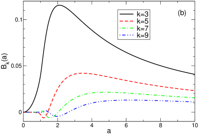
Figure 1: The functions $B_{k}(a)$ for (a) $k=1$ and (b) $k=3,5,7,9$.

Using Eq. (39) we can now present the current (37) in the form of the Fourier expansion over odd frequency harmonics:

$$j_{x}(t)=en_{s}v_{F}\sum_{n=0}^{\infty}\Big{(}\sin[(2n+1)\omega t]{\cal J}_{S}^{(2n+1)}-\cos[(2n+1)\omega t]{\cal J}_{C}^{(2n+1)}\Big{)}.$$ (42)

The first term in the sum, with

$${\cal J}_{S}^{(2n+1)}(\omega\tau,{\cal F}_{\tau})={\cal F}_{\tau}\int^{\infty}_{0}e^{-\xi}\frac{\sin(\omega\tau\xi/2)}{\omega\tau/2}B_{2n+1}\left({\cal F}_{\tau}\frac{\sin(\omega\tau\xi/2)}{\omega\tau/2}\right)\cos[(2n+1)\omega\tau\xi/2]d\xi,$$ (43)

represents the current oscillating “in phase” with the external electric field (19). The second term in (42), with

$${\cal J}_{C}^{(2n+1)}(\omega\tau,{\cal F}_{\tau})={\cal F}_{\tau}\int^{\infty}_{0}e^{-\xi}\frac{\sin(\omega\tau\xi/2)}{\omega\tau/2}B_{2n+1}\left({\cal F}_{\tau}\frac{\sin(\omega\tau\xi/2)}{\omega\tau/2}\right)\sin[(2n+1)\omega\tau\xi/2]d\xi,$$ (44)

represents the current components oscillating “out of phase” with the field $E_{0}\sin\omega t$. In Eqs. (43) and (44) we have introduced a frequency independent field parameter

$${\cal F}_{\tau}=\frac{eE_{0}\tau}{\hbar k_{F}}=\omega\tau{\cal F}_{\omega}$$ (45)

which is more convenient to use analyzing the frequency dependence of the nonlinear response.

Let us analyze the result (42). First, we define an infinite set of generalized “conductivities”

$$\sigma_{(2n+1)\omega,\omega}(\omega\tau,{\cal F}_{\tau})=\frac{en_{s}v_{F}{\cal F}_{\tau}}{E_{0}}\int^{\infty}_{0}e^{-\xi}\frac{\sin(\omega\tau\xi/2)}{\omega\tau/2}B_{2n+1}\left({\cal F}_{\tau}\frac{\sin(\omega\tau\xi/2)}{\omega\tau/2}\right)e^{i(2n+1)\omega\tau\xi/2}d\xi.$$ (46)

Then Eq. (42) assumes the form

$$j_{x}(t)=\sum_{n=0}^{\infty}\Big{(}\sigma^{\prime}_{(2n+1)\omega,\omega}\sin[(2n+1)\omega t]-\sigma^{\prime\prime}_{(2n+1)\omega,\omega}\cos[(2n+1)\omega t]\Big{)}E_{0},$$ (47)

similar to the relation (25). One sees that thus defined functions $\sigma_{(2n+1)\omega,\omega}$ determine the $(2n+1)\omega$-Fourier components of the current responding to the $\omega$-Fourier component of the external field (19). In the low-field limit ${\cal F}_{\tau}\ll 1$ all functions $\sigma_{(2n+1)\omega,\omega}$, except one, vanish, and one gets the conventional Drude result,

$$\sigma_{(2n+1)\omega,\omega}(\omega\tau,{\cal F}_{\tau}\to 0)=\delta_{n0}\frac{\sigma_{0}}{1-i\omega\tau},\ \ \ \sigma_{0}=\frac{n_{s}e^{2}\tau}{(p_{F}/v_{F})}=\frac{e^{2}}{\pi\hbar}\frac{E_{F}\tau}{\hbar},$$ (48)

with the mass $m$ replaced by the effective (electron density dependent) mass of graphene electrons at the Fermi level $p_{F}/v_{F}=E_{F}/v_{F}^{2}$, compare with (24). If the field parameter ${\cal F}_{\tau}$ is finite, the functions $\sigma_{(2n+1)\omega,\omega}(\omega\tau,{\cal F}_{\tau})$, $n>0$, describe the higher (odd) harmonic generation, while the function $\sigma_{\omega,\omega}(\omega\tau,{\cal F}_{\tau})$ determines the intensity dependent response of the system at the incident-wave frequency (Kerr effect). Calculating the averaged (over time) energy dissipated in the system due to the scattering, $\langle\bm{j}\bm{E}\rangle_{t}$,

$$\langle\bm{j}\bm{E}\rangle_{t}=\frac{1}{2}\sigma^{\prime}_{\omega,\omega}(\omega\tau,{\cal F}_{\tau})E_{0}^{2},$$ (49)

we see that the Joule heat is determined by the real part of the function $\sigma_{\omega,\omega}(\omega\tau,{\cal F}_{\tau})$ only; the higher-harmonic conductivities $\sigma_{(2n+1)\omega,\omega}$ do not contribute to $\langle\bm{j}\bm{E}\rangle_{t}$.

Let us rewrite now the conductivities $\sigma_{(2n+1)\omega,\omega}$ in the dimensionless form

$$\sigma_{(2n+1)\omega,\omega}(\omega\tau,{\cal F}_{\tau})=\sigma_{0}{\cal S}_{2n+1}(\omega\tau,{\cal F}_{\tau}),$$ (50)

with

$${\cal S}_{2n+1}(\omega\tau,{\cal F}_{\tau})=\int^{\infty}_{0}e^{-\xi}\frac{\sin(\omega\tau\xi/2)}{\omega\tau/2}B_{2n+1}\left({\cal F}_{\tau}\frac{\sin(\omega\tau\xi/2)}{\omega\tau/2}\right)e^{i(2n+1)\omega\tau\xi/2}d\xi,$$ (51)

and analyze the frequency ($\omega\tau$) and field (${\cal F}_{\tau}$) dependencies of the dimensionless functions ${\cal S}_{2n+1}$.

III Results and their discussion

III.1 Kerr effect

First we consider the function ${\cal S}_{1}(\omega\tau,{\cal F}_{\tau})$ which determines the saturable absorption and Kerr effects. Figure 2 shows the frequency dependence of ${\cal S}_{1}(\omega\tau,{\cal F}_{\tau})$ at a few values of the electric field parameter ${\cal F}_{\tau}$. The curves corresponding to ${\cal F}_{\tau}=0$ are conventional Drude dependencies, since in the limit ${\cal F}_{\tau}\to 0$ one gets ${\cal S}_{1}(\omega\tau,0)=1/(1-i\omega\tau)$. When ${\cal F}_{\tau}$ grows both real and imaginary parts of the conductivity decrease. The suppression of real part ${\cal S}^{\prime}_{1}(\omega\tau,{\cal F}_{\tau})$ at large ${\cal F}_{\tau}$ corresponds to the saturable absorption. In the limit $\omega\tau\to 0$ one gets

$$S_{1}(0,{\cal F}_{\tau})=\int^{\infty}_{0}\xi e^{-\xi}B_{1}({\cal F}_{\tau}\xi)d\xi\approx\left\{\begin{array}[]{lr}1-\frac{3}{4}{\cal F}_{\tau}^{2},&\ {\cal F}_{\tau}\ll 1\\ \frac{4}{\pi{\cal F}_{\tau}},&{\cal F}_{\tau}\gg 1\\ \end{array}\right..$$ (52)

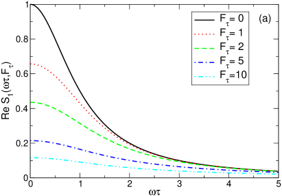
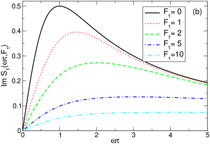
Figure 2: The (a) real and (b) imaginary parts of the function $S_{1}(\omega\tau,{\cal F}_{\tau})$ [Eq. (51), $n=0$] as a function of $\omega\tau$ at different values of the field parameter ${\cal F}_{\tau}$.

Figure 3 illustrates the field dependence of $S_{1}(\omega\tau,{\cal F}_{\tau})$ at several values of the parameter $\omega\tau$. When the field grows, both the real and imaginary parts of $S_{1}(\omega\tau,{\cal F}_{\tau})$ decrease. This reduction is stronger at small values of $\omega\tau$ and much weaker at $\omega\tau\gg 1$. The field and frequency dependencies of the real part of the conductivity, Figure 3a, evidently agree with those recently measured in the experiment of Ref. Mics et al. (2015) (see Fig 1c there).

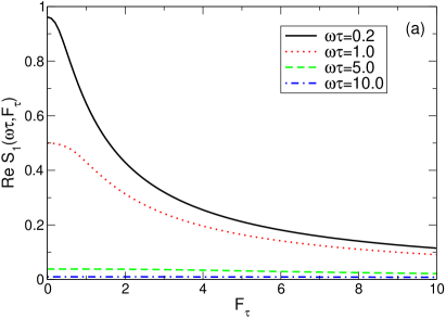
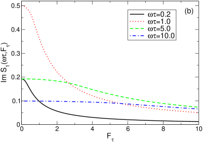
Figure 3: The (a) real and (b) imaginary parts of the function $S_{1}(\omega\tau,{\cal F}_{\tau})$ [Eq. (51), $n=0$] as a function of ${\cal F}_{\tau}$ at different values of the frequency parameter $\omega\tau$.

III.2 Harmonics generation

Now consider the functions ${\cal S}_{2n+1}(\omega\tau,{\cal F}_{\tau})$, $n\geq 1$, responsible for the harmonics generation. Figures 4 – 6 illustrate the frequency dependence of the functions ${\cal S}_{3}(\omega\tau,{\cal F}_{\tau})$, ${\cal S}_{5}(\omega\tau,{\cal F}_{\tau})$ and ${\cal S}_{7}(\omega\tau,{\cal F}_{\tau})$ at a few fixed values of the field parameter ${\cal F}_{\tau}$. Both real and imaginary parts of ${\cal S}_{2n+1}(\omega\tau,{\cal F}_{\tau})$ are quite large at small values of $\omega\tau$ and then quickly decrease (with oscillations) at $\omega\tau\gtrsim 1$. The number of oscillations grows with $n$.

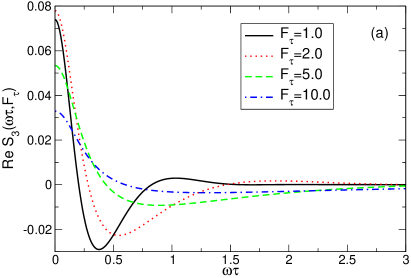
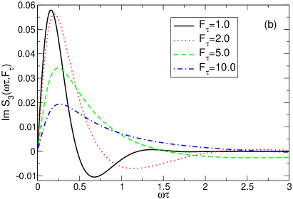
Figure 4: The (a) real and (b) imaginary parts of the function $S_{3}(\omega\tau,{\cal F}_{\tau})$ [Eq. (51), $n=1$] as a function of $\omega\tau$ at different values of the field parameter ${\cal F}_{\tau}$.

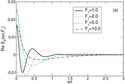
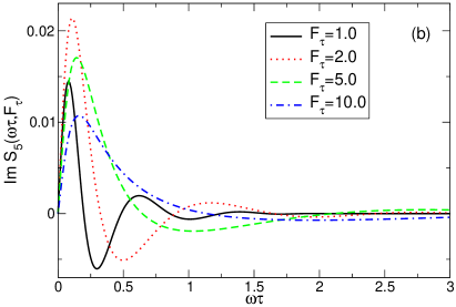
Figure 5: The (a) real and (b) imaginary parts of the function $S_{5}(\omega\tau,{\cal F}_{\tau})$ [Eq. (51), $n=2$] as a function of $\omega\tau$ at different values of the field parameter ${\cal F}_{\tau}$.

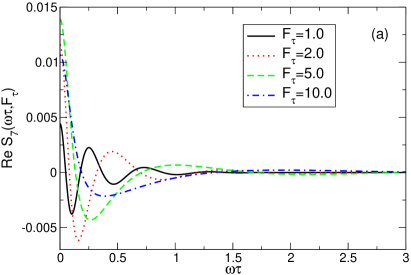
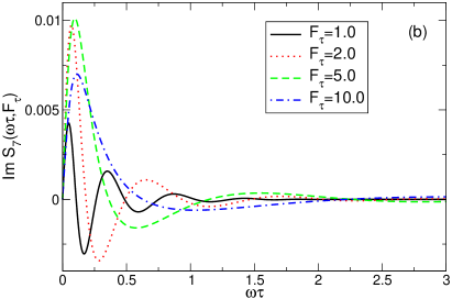
Figure 6: The (a) real and (b) imaginary parts of the function $S_{7}(\omega\tau,{\cal F}_{\tau})$ [Eq. (51), $n=3$] as a function of $\omega\tau$ at different values of the field parameter ${\cal F}_{\tau}$.

Figures 7 – 9 illustrate the field dependence of the functions ${\cal S}_{3}(\omega\tau,{\cal F}_{\tau})$, ${\cal S}_{5}(\omega\tau,{\cal F}_{\tau})$ and ${\cal S}_{7}(\omega\tau,{\cal F}_{\tau})$ at a few fixed values of the frequency $\omega\tau$. The most interesting features seen on these plots are: (a) the absolute values of the functions ${\cal S}_{2n+1}(\omega\tau,{\cal F}_{\tau})$ at $\omega\tau\lesssim 1$ are much larger than those at $\omega\tau\gg 1$, (b) while at small values of the field ${\cal F}_{\tau}\ll 1$ the values of ${\cal S}_{2n+1}(\omega\tau,{\cal F}_{\tau})$ are very small and substantially decrease with the index $n$, at ${\cal F}_{\tau}\gtrsim 1$ all quantities ${\cal S}_{2n+1}(\omega\tau,{\cal F}_{\tau})$ substantially grow and the scale of the functions ${\cal S}_{2n+1}(\omega\tau,{\cal F}_{\tau})$ with different $n$ becomes quite comparable with each other. The last finding is very important. It shows that, while the perturbative solutions, obtained at ${\cal F}_{\tau}\ll 1$, predict very weak amplitudes of the harmonics with $n\gg 1$, the non-perturbative solution shows that at ${\cal F}_{\tau}\gtrsim 1$ all higher harmonics are quite comparable in their amplitude (this is illustrated in Figure 10). The crucial condition for observation of higher harmonics at microwave/terahertz frequencies ($\omega\tau\lesssim 1$) is thus ${\cal F}_{\tau}\gtrsim 1$. The condition ${\cal F}_{\tau}>1$ can be rewritten as

$$\frac{E_{0}(\textrm{kV/cm})\textrm{ }\tau(\textrm{ps})}{\sqrt{n_{s}(10^{12}\textrm{ cm}^{-2})}}>1.16,$$ (53)

i.e. at $\tau\simeq 1$ ps and the density $\simeq 10^{11}-10^{12}$ cm^-2 the field of order of one to few kV/cm is already “strong” in the sense that ${\cal F}_{\tau}\gtrsim 1$ and the higher harmonics (3rd, 5th, 7th, 9th) become observable.

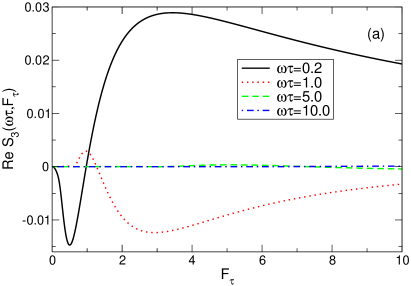
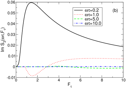
Figure 7: The (a) real and (b) imaginary parts of the function $S_{3}(\omega\tau,{\cal F}_{\tau})$ [Eq. (51), $n=1$] as a function of ${\cal F}_{\tau}$ at different values of the frequency parameter $\omega\tau$.

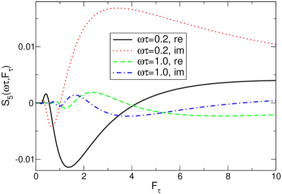
Figure 8: The real and imaginary parts of the function $S_{5}(\omega\tau,{\cal F}_{\tau})$ [Eq. (51), $n=2$] as a function of ${\cal F}_{\tau}$ at different values of the frequency parameter $\omega\tau$.

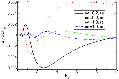
Figure 9: The real and imaginary parts of the function $S_{7}(\omega\tau,{\cal F}_{\tau})$ [Eq. (51), $n=3$] as a function of ${\cal F}_{\tau}$ at different values of the frequency parameter $\omega\tau$.

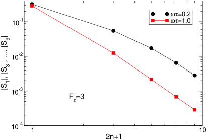
Figure 10: The absolute values of the functions $|S_{2n+1}(\omega\tau,{\cal F}_{\tau})|$, $2n+1=1,3,5,7,9$, as a function of the index $2n+1$ at ${\cal F}_{\tau}=3$ and different values of the frequency parameter $\omega\tau$.

III.3 Is there an optical bistability in graphene?

As we have mentioned in Section I, an optical bistability effect was predicted in a single graphene layer in Ref. Peres et al. (2014). An electromagnetic wave with the frequency $\omega$ and the amplitude $E_{0}$ was assumed to be incident on a single isolated graphene layer and the amplitude of the transmitted wave $E_{t}$ (with the same frequency $\omega$) was calculated. It was shown that the $E_{t}(E_{0})$ dependence is a multivalued function having the $S$-shape.

The result of Ref. Peres et al. (2014) was obtained within the perturbation theory. Now we can check, whether the bistability effect survives if the electromagnetic response of graphene is calculated non-perturbatively.

Similar to Ref. Peres et al. (2014), we consider the incidence of radiation on a single graphene layer placed at the plane $z=0$. The electric and magnetic fields of the wave are then

$$E_{x}(t)=E_{0}^{\omega}e^{-i\omega t}\left\{\begin{array}[]{ll}e^{i\omega z/c}+\rho_{a}e^{-i\omega z/c},&z<0\\ \tau_{a}e^{i\omega z/c},&z>0\\ \end{array}\right.,$$ (54)

$$H_{y}(t)=E_{0}^{\omega}e^{-i\omega t}\left\{\begin{array}[]{ll}e^{i\omega z/c}-\rho_{a}e^{-i\omega z/c},&z<0\\ \tau_{a}e^{i\omega z/c},&z>0\end{array}\right.$$ (55)

where $\rho_{a}$ and $\tau_{a}$ are complex reflection and transmission amplitudes of the wave, and the complex amplitude of the field $E_{0}^{\omega}$ is twice as big as the real amplitude (as in Eq. (19)), $|E_{0}^{\omega}|=2E_{0}$. Applying the conventional boundary conditions at the plane $z=0$ we obtain the transmission ($\tau_{a}$) and reflection ($\rho_{a}$) amplitudes,

$$\tau_{a}=1+\rho_{a}=\frac{1}{1+\frac{2\pi}{c}\sigma_{\omega,\omega}(\omega\tau,{\cal F}_{\tau,z=0})},$$ (56)

as well as the relation between the field at the plane $z=0$ and the field of the incident wave,

$$E_{z=0}^{\omega}=\tau_{a}E_{0}^{\omega}.$$ (57)

Here the field-dependent complex conductivity $\sigma_{\omega,\omega}(\omega\tau,{\cal F}_{\tau})$ is defined in Eq. (46) and the field parameter ${\cal F}_{\tau,z=0}$ is determined by the electric field $E_{z=0}^{\omega}$ at the plane $z=0$. The relation between the electric field parameters ${\cal F}_{\tau,z=0}$ and ${\cal F}_{\tau 0}$ (the latter one is proportional to the absolute value of the incident-wave field, see Eq. (45)) then assumes the form

$${\cal F}_{\tau,z=0}=|\tau_{a}|{\cal F}_{\tau 0}=\frac{{\cal F}_{\tau 0}}{\left|1+\frac{2\pi}{c}\sigma_{\omega,\omega}(\omega\tau,{\cal F}_{\tau,z=0})\right|}.$$ (58)

This can be rewritten as

$${\cal F}_{\tau,z=0}\left|1+\Gamma\tau{\cal S}_{1}(\omega\tau,{\cal F}_{\tau,z=0})\right|={\cal F}_{\tau 0},$$ (59)

where

$$\Gamma=2\frac{e^{2}}{\hbar c}\frac{E_{F}}{\hbar}=2\frac{e^{2}}{\hbar c}v_{F}\sqrt{\pi n_{s}}$$ (60)

is the radiative decay rate first derived in Ref. Mikhailov and Ziegler (2008) (see Eq. (24) there). Figure 11 shows the ratio of the radiative decay rate to the scattering relaxation rate $\Gamma\tau=\Gamma/\gamma$ at different values of the electron density $n_{s}$ and the scattering time $\tau$. The larger is the electron density and their mobility, the bigger is the parameter $\Gamma\tau$.

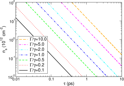
Figure 11: The ratio $\Gamma/\gamma=\Gamma\tau$ of the radiative decay rate $\Gamma$ to the scattering relaxation rate $\gamma$ at different values of $\tau$ (in ps) and of the electron density $n_{s}$ (in units of $10^{12}$ cm^-2).

Now consider the relation (59) between the field parameters ${\cal F}_{\tau 0}$ (proportional to the electric field of the incident wave) and ${\cal F}_{\tau,z=0}$ (proportional to the electric field at the plane $z=0$). The dependence ${\cal F}_{\tau,z=0}({\cal F}_{\tau 0})$ is shown in Figure 12. One sees that, if $\Gamma/\gamma\lesssim 1$, the difference between ${\cal F}_{\tau,z=0}$ and ${\cal F}_{\tau 0}$ is very small. If $\Gamma/\gamma\gg 1$, such a difference does exist: at small values of the field the parameter ${\cal F}_{\tau,z=0}$ grows substantially slower than ${\cal F}_{\tau 0}$; when the field gets stronger, the parameter ${\cal F}_{\tau,z=0}$ grows together with ${\cal F}_{\tau 0}$ with the slope $d{\cal F}_{\tau,z=0}/d{\cal F}_{\tau 0}\simeq 1$. The difference between the field at $z=0$ and the incident-wave field is more pronounced at $\omega\tau\ll 1$. This behavior can be understood by analyzing the formulas (59) and (52) [the expansion (52) is valid at $\omega\tau\ll 1$]. At ${\cal F}_{\tau,z=0}\ll 1$ the function ${\cal S}_{1}\approx 1$ and we get from (59)

$${\cal F}_{\tau,z=0}\approx\frac{{\cal F}_{\tau 0}}{1+\Gamma/\gamma},\ \ \ \omega\tau\ll 1,\ {\cal F}_{\tau,z=0}\ll 1;$$ (61)

if ${\cal F}_{\tau,z=0}\gg 1$ the function ${\cal S}_{1}\approx 4/\pi{\cal F}_{\tau,z=0}$ and we get

$${\cal F}_{\tau,z=0}={\cal F}_{\tau 0}-\frac{4\Gamma}{\pi\gamma},\ \ \ \omega\tau\ll 1,\ {\cal F}_{\tau,z=0}\gg 1.$$ (62)

The asymptotes (61) and (62) (to the curve with $\Gamma/\gamma=10$) are shown in Figure 12(a) by thin blue lines.

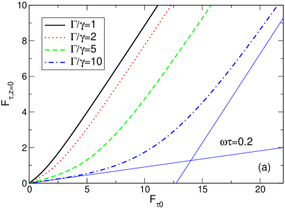
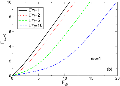
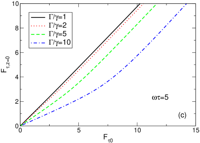
Figure 12: The field parameter ${\cal F}_{\tau,z=0}$ related to the electric field at the plane $z=0$ as a function of the field parameter ${\cal F}_{\tau 0}$ related to the electric field of the incident wave at (a) $\omega\tau=0.2$, (b) $\omega\tau=1$ and (c) $\omega\tau=5$ and at a few different values of the ratio $\Gamma/\gamma$. The thin blue lines in (a) show the asymptotes (61) and (62) to the curve with $\Gamma/\gamma=10$.

The “optical bistability” effect predicted in Ref. Peres et al. (2014) is not seen in Figure 12 at all (small and large) values of both parameters $\omega\tau$ and $\Gamma/\gamma$. Since in Ref. Peres et al. (2014) the problem was solved within the perturbation theory, by expanding the conductivity in powers of the electric field up to $O(E^{4})$, it is reasonable to assume that the reason of the disagreement is related to the use of this expansion. To check this, we have expanded the function ${\cal S}_{1}(\omega\tau,{\cal F}_{\tau,z=0})$ in powers of the electric field up to the same order as it was done in Ref. Peres et al. (2014) (see Appendix B) and obtained the result shown in Figure 13. The perturbation-theory solution does lead to the multi-valued, $S$-shaped dependencies of the output-input characteristics (as seen below, the intensity of the transmitted and the incident light is proportional to $|{\cal F}_{\tau,z=0}|^{2}$ and $|{\cal F}_{\tau 0}|^{2}$, respectively), but this “bistability” disappears if the problem is solved exactly.

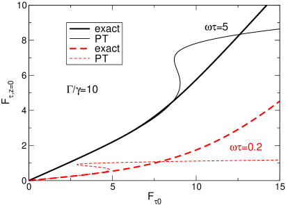
Figure 13: The field parameter ${\cal F}_{\tau,z=0}$ as a function of ${\cal F}_{\tau 0}$ at $\Gamma/\gamma=10$ and two (small and large) values of $\omega\tau$, calculated within the perturbation theory (thin curves, labeled PT), as it was done in Ref. Peres et al. (2014), and non-perturbatively (thick curves, this work). One sees that the “bistability effect” disappears if the problem is solved exactly.

III.4 Scattering of radiation at an isolated graphene layer. Power induced transparency enhancement

To complete the study let us now consider the reflection, transmission and absorption coefficients of the wave incident on an isolated graphene layer (in this Section we consider only the response of graphene at the frequency $\omega$ neglecting the harmonics generation effect). To this end we introduce the intensity of the incident wave ${\cal J}_{i}$ related to the real amplitude $E_{0}$ of the electric field of the incident wave,

$${\cal J}_{i}=\frac{c}{8\pi}E_{0}^{2},$$ (63)

the intensities of the transmitted ${\cal J}_{t}$ and reflected ${\cal J}_{r}$ waves,

$${\cal J}_{t}=\frac{c}{8\pi}E_{0}^{2}\left|\tau_{a}\right|^{2},$$ (64)

$${\cal J}_{r}=\frac{c}{8\pi}E_{0}^{2}\left|\rho_{a}\right|^{2},$$ (65)

and a characteristic intensity value

$${\cal J}_{0}\equiv\frac{c}{8\pi}\left(\frac{\hbar k_{F}}{e\tau}\right)^{2}=\frac{\hbar c}{8e^{2}}\frac{\hbar n_{s}}{\tau^{2}}\approx 1.8\times\frac{n_{s}[10^{12}\mathrm{cm}^{-2}]}{[\tau\mathrm{(ps)}]^{2}}\ \frac{\mathrm{kW}}{\mathrm{cm}^{2}};$$ (66)

using (66) the field parameters ${\cal F}_{\tau 0}$ and ${\cal F}_{\tau,z=0}$ can be written as the ratio of the incident and transmitted waves intencities to ${\cal J}_{0}$:

$${\cal F}_{\tau 0}^{2}=\frac{{\cal J}_{i}}{{\cal J}_{0}},\ \ \ {\cal F}_{\tau,z=0}^{2}=\frac{{\cal J}_{t}}{{\cal J}_{0}}.$$ (67)

The transmission ${\cal T}$, reflection ${\cal R}$ and absorption ${\cal A}$ coefficients then assume the form

$${\cal T}=\frac{{\cal J}_{t}}{{\cal J}_{i}}=\frac{1}{\left|1+\frac{2\pi}{c}\sigma_{\omega,\omega}(\omega\tau,{\cal F}_{\tau,z=0})\right|^{2}}=\frac{1}{\left|1+\frac{\Gamma}{\gamma}{\cal S}_{1}(\omega\tau,{\cal F}_{\tau,z=0})\right|^{2}},$$ (68)

$${\cal R}=\frac{{\cal J}_{r}}{{\cal J}_{i}}=\frac{\left|\frac{\Gamma}{\gamma}{\cal S}_{1}(\omega\tau,{\cal F}_{\tau,z=0})\right|^{2}}{\left|1+\frac{\Gamma}{\gamma}{\cal S}_{1}(\omega\tau,{\cal F}_{\tau,z=0})\right|^{2}},$$ (69)

$${\cal A}=\frac{2\frac{\Gamma}{\gamma}{\cal S}^{\prime}_{1}(\omega\tau,{\cal F}_{\tau,z=0})}{\left|1+\frac{\Gamma}{\gamma}{\cal S}_{1}(\omega\tau,{\cal F}_{\tau,z=0})\right|^{2}}.$$ (70)

The field factor ${\cal F}_{\tau,z=0}$ in Eqs. (68)–(70) depends on ${\cal J}_{t}$, ${\cal F}_{\tau,z=0}=\sqrt{{\cal J}_{t}/{\cal J}_{0}}$, Eq. (67), therefore, in order to find the required dependencies of ${\cal T}$, ${\cal R}$ and ${\cal A}$ on the incident wave intensity ${\cal J}_{i}$, one should first find the relation between ${\cal J}_{t}$ and ${\cal J}_{i}$ from Eq. (68) and then substitute the thus found intensity ${\cal J}_{t}({\cal J}_{i})$ in Eqs. (69) and (70). The functions ${\cal T}$, ${\cal R}$, and ${\cal A}$ in Eqs. (68)–(70) depend on three dimensionless parameters: $\omega\tau$, $\Gamma/\gamma$, and ${\cal J}_{i}/{\cal J}_{0}$.

First, consider the linear response limit ${\cal J}_{i}/{\cal J}_{0}\ll 1$. Then ${\cal F}_{\tau 0}$ and ${\cal F}_{\tau,z=0}$ are small as compared to unity and ${\cal S}_{1}(\omega\tau,{\cal F}_{\tau,z=0}\to 0)\approx 1/(1-i\omega\tau)$. The ${\cal T}$, ${\cal R}$, and ${\cal A}$ coefficients are then

$${\cal T}=\frac{\gamma^{2}+\omega^{2}}{(\gamma+\Gamma)^{2}+\omega^{2}}=1-\frac{\Gamma^{2}+2\gamma\Gamma}{(\gamma+\Gamma)^{2}+\omega^{2}},\ \ \ {\cal J}_{i}/{\cal J}_{0}\ll 1,$$ (71)

$${\cal R}=\frac{\Gamma^{2}}{(\gamma+\Gamma)^{2}+\omega^{2}},\ \ \ {\cal J}_{i}/{\cal J}_{0}\ll 1,$$ (72)

$${\cal A}=\frac{2\Gamma\gamma}{(\gamma+\Gamma)^{2}+\omega^{2}},\ \ \ {\cal J}_{i}/{\cal J}_{0}\ll 1.$$ (73)

The linear-response dependencies (71)–(73) are shown in Figures 14(a)–17(a). One sees that there exist four physically different regimes. If the radiative decay rate is smaller than the scattering rate, $\Gamma\ll\gamma$, Fig. 14, the energy of the incident wave is mainly dissipated into the lattice due to the scattering of electrons by phonons and impurities. The reflection coefficient (red dotted curves) is much smaller than the absorption coefficient (green dashed curves) at all frequencies, and the transmission coefficient is approximately equal to one minus absorption coefficient. At low frequencies ($\omega\tau\ll 1$) ${\cal A}$ is smaller than 50% in this regime (much smaller if $\Gamma\ll\gamma$), while the transmission is larger than 50% (much larger if $\Gamma\ll\gamma$).

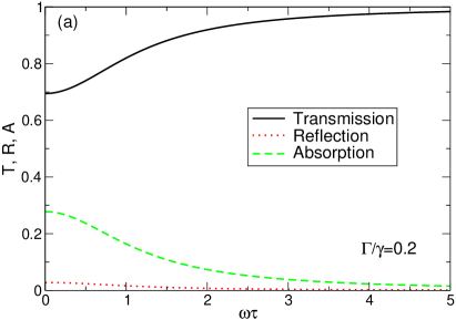
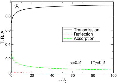
Figure 14: The transmission, reflection and absorption coefficients as a function of (a) the frequency parameter $\omega\tau$ at $\Gamma/\gamma=0.2$ and low intensity of the incident wave ${\cal J}_{i}\to 0$ (the linear response regime), and (b) of the intensity of the incident wave ${\cal J}_{i}/{\cal J}_{0}$ at $\omega\tau=0.2$. At larger values of $\omega\tau$ the behavior of ${\cal T}$, ${\cal R}$, and ${\cal A}$ is similar.

If the incident wave intensity grows, Figure 14(b), the absorption and reflection coefficient fall down while the transmission one substantially grows [in the example of Figure 14(b), $\Gamma/\gamma=0.2$, from 70% at ${\cal J}_{i}/{\cal J}_{0}\to 0$ up to 95% at ${\cal J}_{i}/{\cal J}_{0}=100$ and 97.6% at ${\cal J}_{i}/{\cal J}_{0}=400$]. Figure 14(b) shows the ${\cal J}_{i}$ dependencies of the ${\cal TRA}$ coefficients at $\omega\tau=0.2$; at other frequencies these dependencies are qualitatively the same.

Another interesting case is realized at $\Gamma/\gamma=1$, Figure 15. In this situation, in the linear-response regime and at low frequencies, $\omega\tau\ll 1$, the radiative and dissipative losses are equal, the system absorbs 50% of the incident radiation (this corresponds to the matched load regime), and the transmission and reflection coefficients equal 25% each, Figure 15(a). When the intensity of the incident wave increases, the reflection and absorption coefficients dramatically decrease, while the transmission coefficient substantially grows, Figures 15(b)-(d). For example, at $\omega\tau=0.2$ and ${\cal J}_{i}/{\cal J}_{0}=200$, Figure 15(b), the system absorbs about 15%, reflects less than 0.7% and transmits more than 84%.

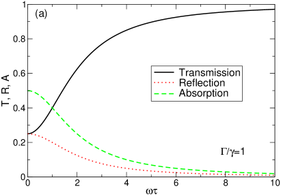
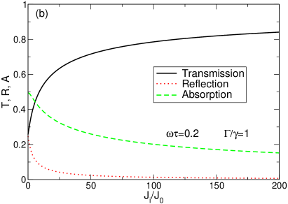
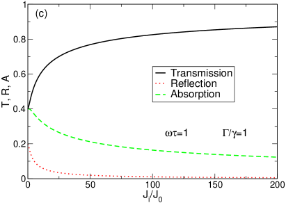
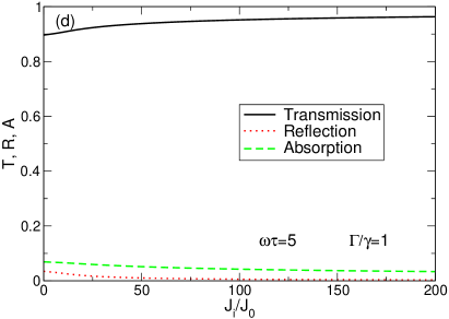
Figure 15: The transmission, reflection and absorption coefficients as a function of (a) the frequency parameter $\omega\tau$ at $\Gamma/\gamma=1$ and low intensity of the incident wave ${\cal J}_{i}\to 0$ (the linear response regime), and of the intensity of the incident wave ${\cal J}_{i}/{\cal J}_{0}$ at (b) $\omega\tau=0.2$, (c) $\omega\tau=1$, and (d) $\omega\tau=5$.

The third interesting case is analyzed in Figure 16. Here $\Gamma=2\gamma$ and the linear-response reflection and absorption coefficients are equal at all frequencies (at least in the Drude model), Figure 16(a). At $\omega\tau\ll 1$ the graphene layer absorbs and reflects about 44.4% and transmits $\sim 11.1$%. When the incident wave intensity grows, the behavior of the ${\cal TRA}$-coefficients differs from that one in the two previous cases. The reflection coefficient quickly falls down as before (red dotted curves in Figures 16(b)–(d)) reaching the values below 1-2% at ${\cal J}_{i}/{\cal J}_{0}\gtrsim 200$. But the behavior of ${\cal A}$ is different. At small values of ${\cal J}_{i}/{\cal J}_{0}$ it first grows up reaching at small frequencies $\sim 50$% and only after that falls down. This growing effect is especially pronounced at $\omega\tau\lesssim 1$, Figs. 16(b)–(c). The transmission coefficient continuously grows with ${\cal J}_{i}/{\cal J}_{0}$ at all frequencies reaching $\sim 80$% at $\omega\tau\lesssim 1$ and ${\cal J}_{i}/{\cal J}_{0}\sim 400$, Figs. 16(b)–(c), and even $\sim 95$% at higher frequencies, Fig. 16(d).

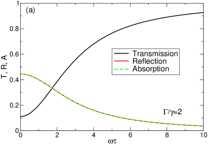
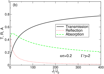
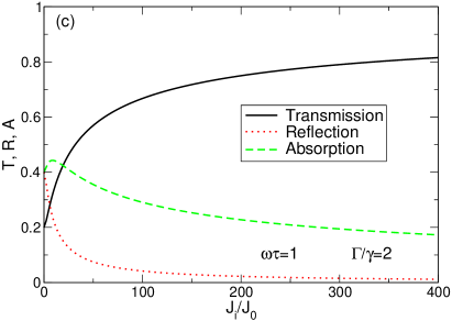
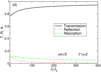
Figure 16: The transmission, reflection and absorption coefficients as a function of (a) the frequency parameter $\omega\tau$ at $\Gamma/\gamma=2$ and low intensity of the incident wave ${\cal J}_{i}\to 0$ (the linear response regime), and of the intensity of the incident wave ${\cal J}_{i}/{\cal J}_{0}$ at (b) $\omega\tau=0.2$, (c) $\omega\tau=1$, and (d) $\omega\tau=5$.

Finally, Figure 17 shows the transmission, reflection and absorption coefficients at $\Gamma\gg\gamma$, when the radiative losses substantially exceed the dissipative losses ($\Gamma/\gamma=5$ in this Figure). Such a situation is realized when either the density or the mobility of the electrons (or both) are large. In this case the transmission coefficient of the 2D layer, in the linear response regime ${\cal J}_{i}\to 0$, is very small at low frequencies $\omega\tau\ll 1$, see Figure 17(a). The energy of the incident wave is either reflected or absorbed, with ${\cal R}/{\cal A}=\Gamma/2\gamma\gg 1$. In the illustrative example of Figure 17 ($\Gamma/\gamma=5$) the layer transmits, at low frequencies, less than 3% and reflects almost 70%.

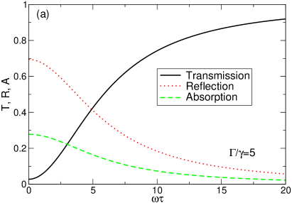
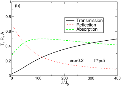
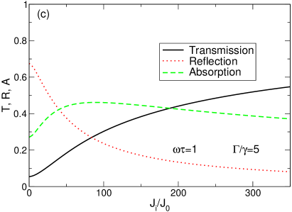
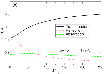
Figure 17: The transmission, reflection and absorption coefficients as a function of (a) the frequency parameter $\omega\tau$ at $\Gamma/\gamma=5$ and low intensity of the incident wave ${\cal J}_{i}\to 0$ (the linear response regime), and of the intensity of the incident wave ${\cal J}_{i}/{\cal J}_{0}$ at (b) $\omega\tau=0.2$, (c) $\omega\tau=1$, and (d) $\omega\tau=5$.

When the intensity ${\cal J}_{i}$ increases, the absorption coefficient first grows up, from $\sim 28$% up to 50% at $\omega\tau\ll 1$, in the example of Figure 17(b), and then falls down at ${\cal J}_{i}\to\infty$. The reflection coefficient falls down with the growing ${\cal J}_{i}$ as in all considered cases. The transmission coefficient continuously increases with ${\cal J}_{i}$, from just a few percent up to 50–80% dependent on the frequency and the intensity ${\cal J}_{i}$.

Thus, in all considered cases the reflection coefficient strongly decreases while the transmission coefficient strongly increases with the growing intensity ${\cal J}_{i}$. The absorption coefficient either monotonously falls down with ${\cal J}_{i}$ at small values of $\Gamma/\gamma$, or first grows and then decreases at large values of $\Gamma/\gamma$. The bistability behavior of the coefficients ${\cal T}$, ${\cal R}$, ${\cal A}$, as a function of ${\cal J}_{i}/{\cal J}_{0}$ is never observed in agreement with results of Section III.3.

IV Summary and conclusions

To summarize, we have theoretically studied the nonlinear electrodynamic response of graphene at low (microwave, terahertz) frequencies, $\hbar\omega\lesssim 2E_{F}$, not using the perturbative theory. We have defined a set of generalized, electric field dependent conductivities $\sigma_{(2n+1)\omega,\omega}(\omega\tau,{\cal F}_{\tau})$, Eq. (46), which determine the current response of graphene at the frequency harmonics $(2n+1)\omega$ if the incident electromagnetic radiation is characterized by a single harmonic $\omega$. We have investigated the conductivities $\sigma_{(2n+1)\omega,\omega}(\omega\tau,{\cal F}_{\tau})$ as functions of the frequency parameter $\omega\tau$ and of the external electric field parameter ${\cal F}_{\tau}$, Eq. (45). We have shown that, while at low fields, at ${\cal F}_{\tau}\lesssim 1$, the higher harmonics amplitudes fall down very strongly with the harmonics number $n$ (proportional to ${\cal F}_{\tau}^{n}$), at higher fields, ${\cal F}_{\tau}\gtrsim 1$, the higher harmonics have much larger relative amplitudes $\propto 1/n$.

We have also investigated the scattering-of-radiation problem and studied the transmission, reflection and absorption coefficients of the monochromatic radiation as a function of the frequency ($\omega\tau$), of the ratio $\Gamma/\gamma$ of the radiative decay rate $\Gamma$ to the scattering rate $\gamma$, and of the dimensionless intensity ${\cal J}_{i}/{\cal J}_{0}$, where the characteristic power density in graphene is defined in Eq. (66). We have found that at large values of ${\cal J}_{i}/{\cal J}_{0}$, the reflection and absorption coefficients strongly fall down, while the transmission of graphene substantially grows and tends to 80-90% even if at low intensities the layer mainly reflected the radiation (at large values of $\Gamma/\gamma$) and the transmission consisted of only a few percent, see, e.g., Figures 16–17. A strong transparency enhancement effect is thus the case in graphene at large values of the incident wave power.

We have shown that the optical bistability effect, predicted within the perturbation theory in Ref. Peres et al. (2014), disappears if to solve the problem non-perturbatively. It should be noticed that in Ref. Sharif et al. (2016a) the authors claimed not only to predict but also to experimentally observe the bi- and multistability effect in exfoliated graphene. However, the theoretical part in this paper is also based on a perturbative (third-order) approach. As for the experimental data (Fig. 10 in Ref. Sharif et al. (2016a)), they only demonstrate a slight difference of the output-vs-input optical characteristics at the growing and decreasing input power, which does not actually look as a strong and sharp hysteresis that would be expected if the true bistability was the case.

The presented theory substantially contributes to the further understanding of the nonlinear electrodynamic properties of graphene, now within the non-perturbative approach, and paves new ways to the development of nonlinear graphene-based optoelectronics.

Appendix A Details of solving the Boltzmann equation

In order to derive Eq. (13) we substitute the second term in Eq. (11) into the Fourier expansion (7),

$$f(p_{x},p_{y},t)=\gamma\int_{-\infty}^{\infty}dse^{isp_{x}}\tilde{f}_{0}(s,p_{y})\int_{-\infty}^{t}e^{-\gamma(t-t^{\prime})-is\int_{t^{\prime}}^{t}F(t^{\prime\prime})dt^{\prime\prime}}dt^{\prime}.$$ (74)

Substituting now for $\tilde{f}_{0}(s,p_{y})$ the inverse Fourier transform of (8) and changing the order of integration we obtain

$$f(p_{x},p_{y},t)=\frac{\gamma}{2\pi}\int_{-\infty}^{\infty}dp_{x}^{\prime}f_{0}(p_{x}^{\prime},p_{y})\int_{-\infty}^{t}e^{-\gamma(t-t^{\prime})}dt^{\prime}\int_{-\infty}^{\infty}dse^{is\left(p_{x}-p_{x}^{\prime}-\int_{t^{\prime}}^{t}F(t^{\prime\prime})dt^{\prime\prime}\right)}$$ (75)

The integral over $ds$ gives the delta function, $\int_{-\infty}^{\infty}\dots ds=2\pi\delta\left(p_{x}-p_{x}^{\prime}-\int_{t^{\prime}}^{t}F(t^{\prime\prime})dt^{\prime\prime}\right)$. Then, integrating over $dp_{x}^{\prime}$ we obtain Eq. (13):

$$f(p_{x},p_{y},t)=\gamma\int_{-\infty}^{t}e^{-\gamma(t-t^{\prime})}f_{0}\left(p_{x}-\int_{t^{\prime}}^{t}F(t^{\prime\prime})dt^{\prime\prime},p_{y}\right)dt^{\prime}.$$ (76)

In order to derive (14) from (13) we rewrite now the integral over $dt^{\prime}$ as a sum of two integrals, the first one from $-\infty$ to 0 and the second from 0 to $t$,

$$f(p_{x},p_{y},t)=\gamma\int_{-\infty}^{0}e^{-\gamma(t-t^{\prime})}f_{0}\left(p_{x}-\int_{t^{\prime}}^{t}F(t^{\prime\prime})dt^{\prime\prime},p_{y}\right)dt^{\prime}+\gamma\int_{0}^{t}e^{-\gamma(t-t^{\prime})}f_{0}\left(p_{x}-\int_{t^{\prime}}^{t}F(t^{\prime\prime})dt^{\prime\prime},p_{y}\right)dt^{\prime}.$$ (77)

In the first integral $t^{\prime}<0<t$, and the lower limit in the integral over $dt^{\prime\prime}$ can be replaced by zero. Then the function $f_{0}$ does not depend on $t^{\prime}$, and the integral over $dt^{\prime}$ can be taken. In both integrals the function $F(t^{\prime\prime})$ can be replaced by $\tilde{F}(t^{\prime\prime})$, so that finally we obtain Eq. (14),

$$f(p_{x},p_{y},t) = e^{-\gamma t}f_{0}\left(p_{x}-\int_{0}^{t}\tilde{F}(t^{\prime\prime})dt^{\prime\prime},p_{y}\right)+\gamma\int_{0}^{t}e^{-\gamma(t-t^{\prime})}f_{0}\left(p_{x}-\int_{t^{\prime}}^{t}\tilde{F}(t^{\prime\prime})dt^{\prime\prime},p_{y}\right)dt^{\prime}.$$ (78)

In order to get Eq. (17) from the exact solution (14) we introduce a new variable $\xi=\gamma(t-t^{\prime})$ in the second integral (the first integral vanishes in the limit $\gamma t\to\infty$) and obtain

$$f(p_{x},p_{y},t)_{\gamma t\to\infty} = \int^{\gamma t}_{0}e^{-\xi}f_{0}\left(p_{x}-\int_{t-\xi/\gamma}^{t}\tilde{F}(t^{\prime\prime})dt^{\prime\prime},p_{y}\right)d\xi.$$ (79)

Equation (17) follows from here in the limit $\gamma t\gg 1$.

Appendix B Asymptotes and Taylor expansions of the functions $B_{2n+1}(a)$ and of the conductivity $\sigma_{\omega,\omega}(\omega\tau,{\cal F}_{\tau})$

The hypergeometric function ${}_{2}F_{1}(\alpha,\beta,\gamma;z)$ which enters the definition (41) of the functions $B_{2n+1}(a)$ is determined by the series

$${}_{2}F_{1}(\alpha,\beta,\gamma;z)=\sum_{n=0}^{\infty}\frac{(\alpha)_{n}(\beta)_{n}}{(\gamma)_{n}}\frac{z^{n}}{n!}=1+\frac{\alpha\beta}{\gamma}\frac{z}{1}+\frac{\alpha(\alpha+1)\beta(\beta+1)}{\gamma(\gamma+1)}\frac{z^{2}}{2!}+\dots$$ (80)

Both at $a\ll 1$ and at $a\gg 1$ the last argument ($z$) of this function is small, therefore to calculate the asymptotes of $B_{2n+1}(a)$ we can use a finite number of terms in the expansion (80). This gives the following behavior of the functions $B_{2n+1}(a)$ at large and small values of the argument $a$. At $a\gg 1$ we obtain

$$B_{2n+1}(a) \approx \frac{4}{\pi a}\int_{0}^{\pi/2}\sin[(2n+1)x]dx=\frac{4}{\pi(2n+1)a},\ \ \ a\gg 1.$$ (81)

If $a\ll 1$ we get

$$B_{1}(a)\approx 1-\frac{3}{2^{5}}a^{2}-\frac{5}{2^{9}}a^{4}+O(a^{6}),$$ (82)

$$B_{3}(a)\approx\frac{1}{2^{5}}a^{2}+\frac{5}{2^{10}}a^{4}+O(a^{6}),$$ (83)

$$B_{5}(a)\approx-\frac{1}{2^{10}}a^{4}-\frac{35}{2^{16}}a^{6}+O(a^{8}),$$ (84)

$$B_{7}(a)\approx\frac{5}{2^{16}}a^{6}+\frac{315}{2^{22}}a^{8}+O(a^{10}).$$ (85)

In order to find the Taylor expansion of the conductivity $\sigma_{\omega,\omega}(\omega\tau,{\cal F}_{\tau})=\sigma_{0}{\cal S}_{1}(\omega\tau,{\cal F}_{\tau})$, defined in (50) we substitute the expansion (82) in the definition of the function ${\cal S}_{1}(\omega\tau,{\cal F}_{\tau})$ and obtain, after straightforward calculations:

$${\cal S}_{1}(\omega\tau,{\cal F}_{\tau}) = \int^{\infty}_{0}e^{-\xi}\frac{\sin(\omega\tau\xi/2)}{\omega\tau/2}B_{1}\left({\cal F}_{\tau}\frac{\sin(\omega\tau\xi/2)}{\omega\tau/2}\right)e^{i\omega\tau\xi/2}d\xi$$ (86)

$$\approx \int^{\infty}_{0}e^{-\xi}\frac{\sin(\omega\tau\xi/2)}{\omega\tau/2}\left[1-\frac{3}{32}\left({\cal F}_{\tau}\frac{\sin(\omega\tau\xi/2)}{\omega\tau/2}\right)^{2}-\frac{5}{512}\left({\cal F}_{\tau}\frac{\sin(\omega\tau\xi/2)}{\omega\tau/2}\right)^{4}+\dots\right]e^{i\omega\tau\xi/2}d\xi$$

$$= \frac{1}{1-i\omega\tau}-\frac{9}{16}{\cal F}_{\tau}^{2}\frac{1}{(1-2i\omega\tau)[1+(\omega\tau)^{2}]}-\frac{75}{64}{\cal F}_{\tau}^{4}\frac{1}{(1-3i\omega\tau)[1+(\omega\tau)^{2}][1+(2\omega\tau)^{2}]}+O\left({\cal F}_{\tau}^{6}\right).$$

References

- Castro Neto et al. (2009) A. H. Castro Neto, F. Guinea, N. M. R. Peres, K. S. Novoselov, and A. K. Geim, “The electronic properties of graphene,” Rev. Mod. Phys. 81, 109–162 (2009).
- Mikhailov (2007) S. A. Mikhailov, “Non-linear electromagnetic response of graphene,” Europhys. Lett. 79, 27002 (2007).
- Dragoman et al. (2010) M. Dragoman, D. Neculoiu, G. Deligeorgis, G. Konstantinidis, D. Dragoman, A. Cismaru, A. A. Muller, and R. Plana, “Millimeter-wave generation via frequency multiplication in graphene,” Appl. Phys. Lett. 97, 093101 (2010).
- Bykov et al. (2012) A. Y. Bykov, T. V. Murzina, M. G. Rybin, and E. D. Obraztsova, “Second harmonic generation in multilayer graphene induced by direct electric current,” Phys. Rev. B 85, 121413(R) (2012).
- Kumar et al. (2013) N. Kumar, J. Kumar, C. Gerstenkorn, R. Wang, H.-Y. Chiu, A. L. Smirl, and H. Zhao, “Third harmonic generation in graphene and few-layer graphite films,” Phys. Rev. B 87, 121406(R) (2013).
- Hong et al. (2013) S.-Y. Hong, J. I. Dadap, N. Petrone, P.-C. Yeh, J. Hone, and R. M. Osgood, Jr., “Optical third-harmonic generation in graphene,” Phys. Rev. X 3, 021014 (2013).
- An et al. (2013) Y. Q. An, F. Nelson, J. U. Lee, and A. C. Diebold, “Enhanced optical second-harmonic generation from the current-biased graphene/SiO2/Si(001) structure,” Nano Lett. 13, 2104–2109 (2013).
- An et al. (2014) Y. Q. An, J. E. Rowe, D. B. Dougherty, J. U. Lee, and A. C. Diebold, “Optical second-harmonic generation induced by electric current in graphene on Si and SiC substrates,” Phys. Rev. B 89, 115310 (2014).
- Lin et al. (2014) K.-H. Lin, S.-W. Weng, P.-W. Lyu, T.-R. Tsai, and W.-B. Su, “Observation of optical second harmonic generation from suspended single-layer and bi-layer graphene,” Appl. Phys. Lett. 105, 151605 (2014).
- Hendry et al. (2010) E. Hendry, P. J. Hale, J. J. Moger, A. K. Savchenko, and S. A. Mikhailov, “Coherent nonlinear optical response of graphene,” Phys. Rev. Lett. 105, 097401 (2010).
- Hotopan et al. (2011) G. Hotopan, S. Ver Hoeye, C. Vazquez, R. Camblor, M. Fernández, F. Las Heras, P. Álvarez, and R. Menéndez, “Millimeter wave microstrip mixer based on graphene,” Progress In Electromagnetic Research 118, 57–69 (2011).
- Gu et al. (2012) T. Gu, N. Petrone, J. F. McMillan, A. van der Zande, M. Yu, G. Q. Lo, D. L. Kwong, J. Hone, and C. W. Wong, “Regenerative oscillation and four-wave mixing in graphene optoelectronics,” Nature Photonics 6, 554–559 (2012).
- Zhang et al. (2012) H. Zhang, S. Virally, Q. L. Bao, L. K. Ping, S. Massar, N. Godbout, and P. Kockaert, “Z-scan measurement of the nonlinear refractive index of graphene,” Optics Letters 37, 1856–1858 (2012).
- Popa et al. (2010) D. Popa, Z. Sun, F. Torrisi, T. Hasan, F. Wang, and A. C. Ferrari, “Sub 200 fs pulse generation from a graphene mode-locked fiber laser,” Appl. Phys. Lett. 97, 203106 (2010).
- Popa et al. (2011) D. Popa, Z. Sun, T. Hasan, F. Torrisi, F. Wang, and A. C. Ferrari, “Graphene Q-switched, tunable fiber laser,” Appl. Phys. Lett. 98, 073106 (2011).
- Vermeulen et al. (2016) N. Vermeulen, D. Castelló-Lurbe, J. L. Cheng, I. Pasternak, A. Krajewska, T. Ciuk, W. Strupinski, H. Thienpont, and J. Van Erps, “Negative Kerr nonlinearity of graphene as seen via chirped-pulse-pumped self-phase modulation,” Phys. Rev. Applied 6, 044006 (2016).
- Constant et al. (2016) T. J. Constant, S. M. Hornett, D. E. Chang, and E. Hendry, “All-optical generation of surface plasmons in graphene,” Nat. Phys. 12, 124–127 (2016).
- Mics et al. (2015) Z. Mics, K.-J. Tielrooij, K. Parvez, S. A. Jensen, I. Ivanov, X. Feng, K. Müllen, M. Bonn, and D. Turchinovich, “Thermodynamic picture of ultrafast charge transport in graphene,” Nature Commun. 6, 7655 (2015).
- Mikhailov and Ziegler (2008) S. A. Mikhailov and K. Ziegler, “Non-linear electromagnetic response of graphene: Frequency multiplication and the self-consistent field effects,” J. Phys. Condens. Matter 20, 384204 (2008).
- Mikhailov (2009a) S. A. Mikhailov, “Non-linear graphene optics for terahertz applications,” Microelectron. J. 40, 712–715 (2009a).
- Mikhailov (2009b) S. A. Mikhailov, “Nonlinear cyclotron resonance of a massless quasiparticle in graphene,” Phys. Rev. B 79, 241309(R) (2009b).
- Dean and van Driel (2009) J. J. Dean and H. M. van Driel, “Second harmonic generation from graphene and graphitic film,” Appl. Phys. Lett. 95, 261910 (2009).
- Dean and van Driel (2010) J. J. Dean and H. M. van Driel, “Graphene and few-layer graphite probed by second-harmonic generation: Theory and experiment,” Phys. Rev. B 82, 125411 (2010).
- Ishikawa (2010) K. L. Ishikawa, “Nonlinear optical response of graphene in time domain,” Phys. Rev. B 82, 201402 (2010).
- Mikhailov (2011) S. A. Mikhailov, “Theory of the giant plasmon-enhanced second-harmonic generation in graphene and semiconductor two-dimensional electron systems,” Phys. Rev. B 84, 045432 (2011).
- Jafari (2012) S. A. Jafari, “Nonlinear optical response in gapped graphene,” J. Phys. Condens. Matter 24, 205802 (2012).
- Mikhailov and Beba (2012) S. A. Mikhailov and D. Beba, “Nonlinear broadening of the plasmon linewidth in a graphene stripe,” New J. Phys. 14, 115024 (2012).
- Avetissian et al. (2013) H. K. Avetissian, G. F. Mkrtchian, K. G. Batrakov, S. A. Maksimenko, and A. Hoffmann, “Multiphoton resonant excitations and high-harmonic generation in bilayer graphene,” Phys. Rev. B 88, 165411 (2013).
- Mikhailov (2013) S. A. Mikhailov, “Electromagnetic nonlinearities in graphene,” in Carbon nanotubes and graphene for photonic applications, edited by Shinji Yamashita, Yahachi Saito, and Jong Hyun Choi (Woodhead Publishing Limited, Oxford, Cambridge, Philadelphia, New Delhi, 2013) Chap. 7, pp. 171–219.
- Cheng et al. (2014a) J. L. Cheng, N. Vermeulen, and J. E. Sipe, “Third order optical nonlinearity of graphene,” New J. Phys. 16, 053014 (2014a).
- Cheng et al. (2014b) J. L. Cheng, N. Vermeulen, and J. E. Sipe, “Dc current induced second order optical nonlinearity in graphene,” Optics Express 22, 15868–15876 (2014b).
- Yao et al. (2014) X. Yao, M. Tokman, and A. Belyanin, “Efficient nonlinear generation of THz plasmons in graphene and topological insulators,” Phys. Rev. Lett. 112, 055501 (2014).
- Smirnova et al. (2014) D. A. Smirnova, I. V. Shadrivov, A. E. Miroshnichenko, A. I. Smirnov, and Y. S. Kivshar, “Second-harmonic generation by a graphene nanoparticle,” Phys. Rev. B 90, 035412 (2014).
- Peres et al. (2014) N. M. R. Peres, Y. V. Bludov, J. E. Santos, A.-P. Jauho, and M. I. Vasilevskiy, “Optical bistability of graphene in the terahertz range,” Phys. Rev. B 90, 125425 (2014).
- Cox and de Abajo (2014) J. D. Cox and F. J. G. de Abajo, “Electrically tunable nonlinear plasmonics in graphene nanoislands,” Nat. Commun. 5, 5725 (2014).
- Cox and de Abajo (2015) J. D. Cox and F. J. G. de Abajo, “Plasmon-enhanced nonlinear wave mixing in nanostructured graphene,” ACS Photonics 2, 306–312 (2015).
- Savostianova and Mikhailov (2015) N. A. Savostianova and S. A. Mikhailov, “Giant enhancement of the third harmonic in graphene integrated in a layered structure,” Appl. Phys. Lett. 107, 181104 (2015).
- Cheng et al. (2015) J. L. Cheng, N. Vermeulen, and J. E. Sipe, “Third-order nonlinearity of graphene: Effects of phenomenological relaxation and finite temperature,” Phys. Rev. B 91, 235320 (2015).
- Cheng et al. (2016a) J. L. Cheng, N. Vermeulen, and J. E. Sipe, “Erratum: Third-order nonlinearity of graphene: Effects of phenomenological relaxation and finite temperature [Phys. Rev. B 91, 235320 (2015)],” Phys. Rev. B 93, 039904(E) (2016a).
- Mikhailov (2016) S. A. Mikhailov, “Quantum theory of the third-order nonlinear electrodynamic effects in graphene,” Phys. Rev. B 93, 085403 (2016).
- Mikhailov et al. (2016) S. A. Mikhailov, N. A. Savostianova, and A. S. Moskalenko, “Negative dynamic conductivity of a current-driven array of graphene nanoribbons,” Phys. Rev. B 94, 035439 (2016).
- Rostami and Polini (2016) H. Rostami and M. Polini, “Theory of third-harmonic generation in graphene: A diagrammatic approach,” Phys. Rev. B 93, 161411(R) (2016).
- Cox et al. (2016) J. D. Cox, I. Silviero, and F. J. G. de Abajo, “Quantum effects in the nonlinear response of graphene plasmons,” ACS NANO 10, 1995–2003 (2016).
- Marini et al. (2016) A. Marini, J. D. Cox, and F. J. G. de Abajo, “Theory of graphene saturable absorption,” arXiv:1605.06499 (2016).
- Sharif et al. (2016a) M. A. Sharif, M. H. M. Ara, B. Ghafary, S. Salmani, and S. Mohajer, “Experimental observation of low threshold optical bistability in exfoliated graphene with low oxidation degree,” Opt. Mater. 53, 80–86 (2016a).
- Sharif et al. (2016b) M. A. Sharif, B. Ghafary, and M. H. M. Ara, “A novel graphene-based electro-optical modulator using modulation instability,” IEEE Photonics Technology Lett. 28, 2897 – 2900 (2016b).
- Cheng et al. (2016b) J. L. Cheng, N. Vermeulen, and J. E. Sipe, “Forbidden second order optical nonlinearity of graphene,” (2016b), arXiv:1609.06413v1.
- Wang et al. (2016) Y. Wang, M. Tokman, and A. Belyanin, “Second-order nonlinear optical response of graphene,” Phys. Rev. B 94, 195442 (2016).
- Tokman et al. (2016) M. Tokman, Y. Wang, I. Oladyshkin, A. R. Kutayiah, and A. Belyanin, “Laser-driven parametric instability and generation of entangled photon-plasmon states in graphene,” Phys. Rev. B 93, 235422 (2016).
- Rostami et al. (2016) H. Rostami, M. I. Katsnelson, and M. Polini, “Theory of plasmonic effects in nonlinear optics: the case of graphene.” (2016), arXiv:1610.04854.
- Glazov and Ganichev (2014) M. M. Glazov and S. D. Ganichev, “High frequency electric field induced nonlinear effects in graphene,” Phys. Rep. 535, 101–138 (2014).
- Hartmann et al. (2014) R. R. Hartmann, J. Kono, and M. E. Portnoi, “Terahertz science and technology of carbon nanomaterials,” Nanotechnology 25, 322001 (2014).
- Romanets and Vasko (2010) P. N. Romanets and F. T. Vasko, “Transient response of intrinsic graphene under ultrafast interband excitation,” Phys. Rev. B 81, 085421 (2010).
- Romanets and Vasko (2011) P. N. Romanets and F. T. Vasko, “Depletion of carriers and negative differential conductivity in intrinsic graphene under a dc electric field,” Phys. Rev. B 83, 205427 (2011).
- Ignatov and Romanov (1976) A. A. Ignatov and Yu. A. Romanov, “Nonlinear electromagnetic properties of semiconductors with a superlattice,” phys. stat. sol. (b) 78, 327–333 (1976).