Upper Minkowski dimension estimates for convex restrictions

Abstract

We show that there are functions $f$ in the Hölder class $C^{\alpha}[0,1]$, $1<\alpha<2$ such that $f|_{A}$ is not convex, nor concave for any $A\subset[0,1]$ with $\operatorname{\overline{dim}_{M}}A>\alpha-1$.

Our earlier result shows that for the typical/generic $f\in C_{1}^{\alpha}[0,1]$, $0\leq\alpha<2$ there is always a set $A\subset[0,1]$ such that $f|_{A}$ is convex and $\operatorname{\overline{dim}_{M}}A=1$.

The analogous statement for monotone restrictions is the following: there are functions $f$ in the Hölder class $C^{\alpha}[0,1]$, $1/2\leq\alpha<1$ such that $f|_{A}$ is not monotone on $A\subset[0,1]$ with $\operatorname{\overline{dim}_{M}}A>\alpha$. This statement is not true for the range of parameters $\alpha<1/2$ and the main theorem of this paper for the parameter range $1<\alpha<3/2$ cannot be obtained by integration of the result about monotone restrictions.

1 Introduction

In an earlier paper [2] we discussed results about convex and monotone restrictions of functions belonging to different Hölder classes. This paper was related to [1], [4], [5], [6] and several others. In [1] and [2] one can read more about the background of these results.

We denote by $\operatorname{dim_{H}}A$, $\operatorname{\overline{dim}_{M}}A$, and $\operatorname{\underline{\mathrm{dim}}_{M}}A$ the Hausdorff, the lower and upper Minkowski (box) dimension of the set $A$, respectively. In [2] we showed that for the generic/typical $f\in C_{1}^{\alpha}[0,1]$, when $0\leq\alpha<1$ if $A\subset[0,1]$ and $f|_{A}$ is monotone then $\operatorname{\underline{\mathrm{dim}}_{M}}A\leq\alpha$. It is rather easy to see that for any $0<\alpha\leq 1$ if $f\in C^{\alpha}[0,1]$ then there exists $A\subset[0,1]$ such that $f|_{A}$ is monotone and $\operatorname{dim_{H}}A\geq\alpha$. According to a result from [1] if $0<\alpha<1$ and $B(t)$ is a fractional Brownian motion of Hurst index $\alpha$ then almost surely $B|_{A}$ is not monotone increasing for any $A$ with $\operatorname{\overline{dim}_{M}}A>\max\{1-\alpha,\alpha\}$. Fractional Brownian motion of Hurst index $\alpha$ belongs to $C^{\alpha-}[0,1]$. In [1] for a dense set of $\widehat{\alpha}$s in $[1/2,1]$ examples of self similar functions $f\in C^{\widehat{\alpha}}[0,1]$ were also provided for which $f|_{A}$ is not monotone for any $A$ with $\operatorname{\overline{dim}_{M}}A>\widehat{\alpha}$. I learned from R. Balka about an unpublished argument of A. Máthé, which implies that for any function $f:[0,1]\to\mathbb{R}$ one can always find a set $A$ such that $f|_{A}$ is monotone and $\operatorname{\overline{dim}_{M}}A\geq 1/2$.

With respect to convex restrictions in [2] we proved that for typical/generic $f\in C_{1}^{\alpha}[0,1]$ (in the sense of Baire category), $0\leq\alpha<2$ there is always a set $A\subset[0,1]$ such that $f|_{A}$ is convex and $\operatorname{\overline{dim}_{M}}A=1$. For generic $f\in C_{1}^{\alpha}[0,1]$, $0<\alpha<2$ we have shown that for any $A\subset[0,1]$ such that $f|_{A}$ is convex, or concave we have $\operatorname{\underline{\mathrm{dim}}_{M}}A\leq\max\{0,\alpha-1\}.$ In this paper we prove that for $1<\alpha<2$ there are functions $f\in C^{\alpha}[0,1]$, such that $f|_{A}$ is not convex, nor concave for any $A\subset[0,1]$ with $\operatorname{\overline{dim}_{M}}A>\alpha-1$. By multiplying with a suitable constant one can obtain functions $f\in C^{\alpha}_{1}[0,1]$ in our example. In [2] we also proved for $1<\alpha\leq 2$ for any $f\in C^{\alpha}[0,1]$ there is always a set $A\subset[0,1]$ such that $\alpha-1=\operatorname{dim_{H}}A\leq\operatorname{\underline{\mathrm{dim}}_{M}}A\leq\operatorname{\overline{dim}_{M}}A$ and $f|_{A}$ is convex, or concave on $A$. This shows that the main result of our current paper is best possible.

It is interesting that for $3/2\leq\alpha<2$ by integrating Fractional Brownian motions of Hurst index $\alpha-1$ one can obtain functions $f\in C^{\alpha-}[0,1]$ with the property that $f|_{A}$ is not convex, nor concave for any $A\subset[0,1]$ with $\operatorname{\overline{dim}_{M}}A>\alpha-1$. By using from [1] the earlier mentioned dense set of $\widehat{\alpha}$s in $[1/2,1]$ taking integrals of the corresponding self-similar functions one can obtain a dense set in $3/2\leq\alpha<2$ and functions $f\in C^{\alpha}[0,1]$ with the property that $f|_{A}$ is not convex, nor concave for any $A\subset[0,1]$ with $\operatorname{\overline{dim}_{M}}A>\alpha-1$. As it was requested by readers of ealier versions of our paper in Proposition 3 we provide some details of this procedure of obtaining convexity results from monotonicity results by integration.

For the parameter range $1\leq\alpha<3/2$ it is not possible to take integrals of functions constructed for monotone restrictions. Fortunately, our proof works for the whole parameter range $(1,2)$. Based on similar ideas the result concerning the case $\alpha=1$ can also be established, though we do not make the lengthy and complicated proof of our paper even longer and more complicated by considering this case as well.

Since the proof is quite complicated and contains quite a few technical details here we want to give the main heuristic idea of our argument.

Figure 1: ${\phi}$, ${\widetilde{f}}$ and $c_{1}$

Suppose $N$ is a fixed sufficiently large even integer. One can consider the function ${\phi}(x)=c_{1}+c_{2}(-1)^{j+1}$ for $x\in[(j-1)/N,j/N]$, $j=1,...,N$. We take its antiderivative ${\widetilde{f}}(x)=\int_{0}^{x}{\phi}(t)dt$. These functions are illustrated on the left half of Figure 1. It is clear that if ${\widetilde{f}}$ is convex on a set $A$ then there are at most two $j$’s for which $[(j-1)/N,j/N]$ contains more than two points of $A$. Though, it may happen that some other intervals contain single points of $A$. See again the left half of Figure 1 where the hollow dots illustrate the correspondig points $(a,{\widetilde{f}}(a)),$ $a\in A$ on the graph of ${\widetilde{f}}$. We will have to consider in our paper functions $f$ which are sufficiently close to ${\widetilde{f}}$. These functions will inherit the property that if $f$ is convex on a set $A$ then there are at most two $j$’s for which $[(j-1)/N,j/N]$ contains more than two points of $A$. In the proof of our theorem this will be behind Claims 12 and 13. The function ${\phi}$ on the left half of Figure 1 is not continuous and we need Hölder $\alpha$ derivative for our function $f$ in Theorem 4. Instead of the discontinuous ${\phi}$ we will use functions ${\phi}$ which are pictured on the right half of Figure 1 and appear in Subsection 3.2, especially in (13). Unfortunately, for these functions there are intervals, where they are not locally constant. We will call these intervals transitional intervals. We also need to deal with the problem that for a bound on the upper box dimension we have to consider all scaling levels with grid intervals of the form $[(j-1)/N^{k},j/N^{k}]$, $k\in\mathbb{N}$, $j\in\{1,...,N^{k}\}$ and verify that for all sufficiently large $k$ if $f$ is convex on $A$ then we do not have too many such grid intervals which contain points of $A$. This means that by subsequent perturbation of the previous functions we define the sequence of functions ${\phi}_{n}$ which will uniformly converge to a Hölder $\alpha$ function $g_{1}$. This function $g_{1}$ is good for our purposes at points where it is “almost locally constant”. However due to the existence of transitional intervals we need a second infinite sequence of modifications yielding the sequence $g_{n}$. These functions $g_{n}$ will converge to a function $g$ and our function $f$ will be the antiderivative of $g$.

The author thanks R. Balka and the unknown referee for the careful reading of the paper and for comments which improved the presentation of the results.

2 Notation and preliminary results

For $\alpha\geq 0$ if $f:[0,1]\to\mathbb{R}$ is $\lfloor\alpha\rfloor$-times differentiable (by definition $f^{(0)}=f$) we put

$${\cal L}_{\alpha}(f)=\sup\Big{\{}\frac{|f^{(\lfloor\alpha\rfloor)}(x)-f^{(\lfloor\alpha\rfloor)}(y)|}{|x-y|^{\{\alpha\}}}:x\not=y,\ x,y\in[0,1]\Big{\}}.$$ (1)

By $C^{0}[0,1]$, or $C[0,1]$ we denote the class of continuous functions on $[0,1]$.

If $0<\alpha<1$ then $f$ is in $C^{\alpha}[0,1]$, if ${\cal L}_{\alpha}(f)<\infty$.

The function $f$ is in $C^{1}[0,1]$ if $f^{{}^{\prime}}$ is continuous on $[0,1]$.

If $1<\alpha<2$ then $f$ is in $C^{\alpha}[0,1]$ if $f$ is differentiable, and $f^{{}^{\prime}}\in C^{\alpha-1}[0,1]$, that is ${\cal L}_{\alpha}(f)<\infty$.

We denote by $C^{\alpha-}[0,1]$ the set of those functions which are in $C^{\beta}[0,1]$ for all $\beta<\alpha$.

For $0\leq\alpha$, $\alpha\not\in\mathbb{N}$, $f$ is in $C_{1}^{\alpha}[0,1]$ if ${\cal L}_{\alpha}(f)\leq 1$, that is $|f^{(\lfloor\alpha\rfloor)}(x)-f^{(\lfloor\alpha\rfloor)}(y)|\leq|x-y|^{\{\alpha\}}$ for all $x,y\in[0,1]$.

Given an integer $N\geq 2$ and a set $A\subset[0,1]$ we put for $k\in\mathbb{Z}$

$${\cal N}_{N,k}(A)=\#\Big{\{}j\in\mathbb{Z}:A\cap\Big{[}\frac{j-1}{N^{k}},\frac{j}{N^{k}}\Big{]}\not=\emptyset\Big{\}}.$$

The upper and lower Minkowski (or box) dimension of $A$ is defined as

$$\operatorname{\overline{dim}_{M}}A=\limsup_{k\to\infty}\frac{\log{\cal N}_{N,k}(A)}{k\log N}\text{ and }\operatorname{\underline{\mathrm{dim}}_{M}}A=\liminf_{k\to\infty}\frac{\log{\cal N}_{N,k}(A)}{k\log N}.$$ (2)

It is well-known that for any $N$ we obtain the same value.

Notation 1.

For sets $A\subset[0,1]$ we put

$${{\cal F}}_{N,k}(A)=\cup\{[(j-1)/N^{k},j/N^{k}]:\ A\cap[(j-1)/N^{k},j/N^{k}]\not=\emptyset\}.$$

Clearly, ${{\cal N}}_{N,k}(A)=\lambda({{\cal F}}_{N,k}(A))\cdot N^{k}.$ (We denote by $\lambda$ the one-dimensional Lebesgue measure.)

The open ball centered at $x$ and of radius $r$ is denoted by $B(x,r)$. The $\alpha$-dimensional Hausdorff measure is denoted by ${\cal H}^{\alpha}$.

We remind the reader to a few facts about iterated function systems. The details can be found in many books, for example in [3]. If $S_{i}$, $i=1,...,N$, $N\geq 2$ is a family of similarities with contraction ratios $c_{i}$ then we talk about an IFS, an iterated function system. The attractor of the IFS is the compact set $F$ satisfying $F=\cup_{i}S_{i}(F)$. The similarity dimension of $F$ is the unique $\alpha$ for which $\sum_{i}c_{i}^{\alpha}=1$. If the IFS satisfies the, so called open set condition then the Hausdorff, the Minkowski and the similarity dimension of $F$ are the same (see for example Theorem 9.3 of [3] ). We recall 4.14. Theorem from [7] by using our notation:

Theorem 2.

If $S_{i}$, $i=1,...,N$ satisfies the open set condition, then the invariant set $F$ is self-similar and $0<{\cal H}^{\alpha}(F)<+\infty$, whence $\alpha=\operatorname{dim_{H}}F$, where $\alpha$ is the unique number for which $\displaystyle\sum_{i}c_{i}^{\alpha}=1.$ Moreover, there are positive and finite numbers $a$ and $b$ such that

$$ar^{\alpha}<{\cal H}^{\alpha}(F\cap B(x,r))<br^{\alpha}\text{ for }x\in F,\ 0<r<1.$$ (3)

In our paper the self similar sets for which this theorem will be applied will satisfy the strong separation condition, that is the sets $S_{i}(F)$ will be disjoint, and hence the open set condition will also be satisfied.

We suppose that $F\subset[0,1]$ is the attractor of an IFS satisfying the open set condition. Estimation (3) will be useful several ways.

If one considers the function ${\phi}(x)={\cal H}^{\alpha}(F\cap[0,x])/{\cal H}^{\alpha}(F)$ then it is easy to deduce from (3) that ${\phi}$ is Hölder-$\alpha$.

On the other hand, using the lefthand-side inequality in (3) it is also easy to see that for fixed $N$ there exists a constant $C_{F}$ such that

$${\cal N}_{N,k}(F)<C_{F}N^{\alpha k}\text{ for any }k\in\mathbb{N}.$$ (4)

Indeed, one needs to observe that if $x\in F\cap[(j-1)/N^{k},j/N^{k}]$ then ${\cal H}^{\alpha}(F\cap[(j-2)/N^{k},(j+1)/N^{k}])\geq{\cal H}^{\alpha}(F\cap B(x,1/N^{k})>a/N^{\alpha k}$.

Readers of earlier versions of this paper asked for more details about “integrating” monotonicity results to obtain convexity estimates. In the proof of the next proposition we provide these details.

Proposition 3.

Suppose $\alpha\in[0,1]$, $g\in C[0,1]$ and $g|_{B}$ is not monotone for any $B\subset[0,1]$ with $\operatorname{\overline{dim}_{M}}B>\alpha$. Put $f(x)=\int_{0}^{x}g(t)dt.$ Then $f|_{A}$ is not convex, nor concave for any $A\subset[0,1]$ with $\operatorname{\overline{dim}_{M}}A>\alpha$.

Proof.

Suppose that $A\subset[0,1]$ is closed and $f|_{A}$ is convex (the concave case is similar and is left to the reader). Denote by ${\cal I}_{A}$ the shortest closed interval containing $A$. One can extend the definition of $f|_{A}$ onto ${\cal I}_{A}$ to obtain a convex function $h$ defined on ${\cal I}_{A}$ and $f|_{A}=h|_{A}$. At two-sided accumulation points $a$ of $A$ we have $h^{\prime}(a)=f^{\prime}(a)=g(a)$. At one-sided accumulation points $a$ of $A$ we have $h^{\prime}_{\pm}(a)=f^{\prime}(a)=g(a)$ where $h^{\prime}_{\pm}(a)=h^{\prime}_{+}(a)$, or $h^{\prime}_{\pm}(a)=h^{\prime}_{-}(a)$ for right, or left accumulation points of $A$, respectively.

Suppose $a$ is an isolated point of $A$. If $a$ is not an endpoint of ${\cal I}_{A}$ then select $c\in A$ and $b\in A$ such that $b<a<c$ and $(b,c)\cap A=\{a\}.$ By the Mean Value Theorem there is $a_{-}\in(b,a)$ and $a_{+}\in(a,c)$ such that

$$f^{\prime}(a_{-})=g(a_{-})=\frac{f(a)-f(b)}{a-b}=\frac{h(a)-h(b)}{a-b},\text{ and }$$

$$f^{\prime}(a_{+})=g(a_{+})=\frac{f(c)-f(a)}{c-a}=\frac{h(c)-h(a)}{c-a}.$$

If $a$ is the left-endpoint of ${\cal I}_{A}$ then we define only $a_{+}$, if $a$ is the right-endpoint of ${\cal I}_{A}$ then we define only $a_{-}$.

Denote by $B$ the set which contains all accumulation points of $A$ and the points $a_{+}$ and $a_{-}$ for isolated points of $A$. Then the convexity of $h$ on ${\cal I}_{A}$ and the above equalities imply that $g$ is montone increasing on $B$ and hence, say for $N=2$ we have

$$\operatorname{\overline{dim}_{M}}B=\limsup_{k\to\infty}\frac{\log{\cal N}_{2,k}(B)}{k\log 2}\leq\alpha.$$

The $1/2^{k}$ grid intervals taken into consideration in ${\cal N}_{2,k}(B)$ cover all accumulation points of $A$ and the points $a_{+}$ and $a_{-}$ corresponding to isolated points of $A$. Hence ${\cal N}_{2,k}(A)\leq 3{\cal N}_{2,k}(B)$. This implies that $\operatorname{\overline{dim}_{M}}A\leq\alpha$. ∎

3 Main result

Theorem 4.

Let $0<\alpha<1$. There exits $f\in C^{1+\alpha}[0,1]$ such that for any $A\subset[0,1]$ with $\operatorname{\overline{dim}_{M}}A>\alpha$ the restriction $f|_{A}$ is neither convex, nor concave.

Remark 5.

Multiplying $f$ by a suitable constant one can achieve $f\in C_{1}^{1+\alpha}[0,1]$ as well. As it was mentioned in the introduction the theorem can be proved for $\alpha=0$ as well, with a suitably modified other, rather technical proof.

Proof.

We will define $g=f^{\prime}\in C^{\alpha}[0,1]$.

A large even integer $N$ will be fixed later.

Before giving the details of the proof we give a list of some notation introduced at different steps. This might be helpful for later reference.

In Subsection 3.1 we introduce the self-similar set $F_{0}$ and the Hölder $\alpha$ function ${\phi}_{0}$, which is constant on the connected components of the open set $G_{0}=[0,1]\setminus F_{0}$. The collection of these connected components of $G_{0}$ are denoted by ${\cal I}_{0}$.

In Subsection 3.2 the functions ${\phi}_{n}$ are defined. These functions are constant on the connected components ($I(a,b,j)$ in (12)) of the open sets $G_{n}=[0,1]\setminus F_{n}$ defined in (16). The connected components of $G_{n}$ are denoted by ${\cal I}_{n}$. These sets are nested, $G_{n+1}\subset G_{n}$. While ${\phi}_{n}$, defined in (13) is constant on the intervals $I(a,b,j)$ there will be some transitional intervals, where ${\phi}_{n}$ is non-constant and linear. These transitional intervals are the connected components of $G_{n}^{\prime}$, defined in (14). The collection of these connected components of $G_{n}^{\prime}$ are denoted by ${\cal I}_{n}^{\prime}$. The sets $G_{n}^{\prime}$ are disjoint.

In Subsection 3.3 the function $g_{1}$ is defined. Its transitional intervals, denoted by ${\cal I}_{T,1}^{\prime}$ are the connected components of $G^{\prime}_{T,1}=\cup_{n=1}^{\infty}G_{n}^{\prime}.$

In Subsection 3.4 the functions $g_{n}$ are defined for $n\geq 2$. The corresponding transitional intervals are denoted by ${\cal I}_{T,n}^{\prime}$. They are the connected components of $G^{\prime}_{T,n}.$ The sets $G^{\prime}_{T,n}$ are also nested, they satisfy $G^{\prime}_{T,n+1}\subset G^{\prime}_{T,n}.$ The function $g$ will be the limit of the functions $g_{n}$.

In Subsection 3.5 the Hölder property of $g$ and of its antiderivative $f$ is verified.

In Subsection 3.6 we define and estimate ${\cal S}(G,\alpha)$ to measure the size of the sets $G_{n}^{\prime}$.

In Subsection 3.7 we give the upper estimate of the upper box dimension of the sets $A$ on which $f$ can be convex, or concave. Here the most important definition is $G^{\prime\prime}_{T,j,k}\subset G^{\prime}_{T,j}$ which contains all transitional intervals of $g_{j}$ which are of length longer than $N^{-k}$. The collection of the connected components of $G^{\prime\prime}_{T,j,k}$ is denoted by ${\cal I}^{\prime\prime}_{T,j,k}$. In Claim 11 we estimate ${{\cal N}}_{N,k}(A\setminus{G}_{T,1,k}^{\prime\prime})$ and in Claim 14 we reduce the general case to this initial one.

3.1 The definition of the self similar set $F_{0}$ and of the Hölder $\alpha$ function ${\phi}_{0}$

Figure 2: $F_{0,1}$

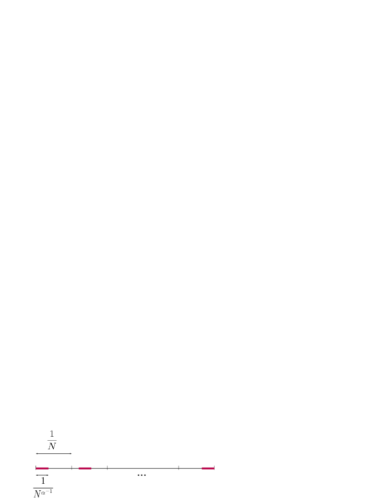
First we select a standard Hölder $\alpha$ function ${\phi}_{0}$ the following way. Let $F_{0,1}$ consist of the following subintervals of $[0,1]$

$$\Big{[}(j-1)\cdot\left(\frac{1}{N}+\frac{1}{N-1}\left(\frac{1}{N}-\frac{1}{N^{\alpha^{-1}}}\right)\right),\hskip 56.9055pt$$ (5)

$$\hskip 56.9055pt(j-1)\cdot\left(\frac{1}{N}+\frac{1}{N-1}\left(\frac{1}{N}-\frac{1}{N^{\alpha^{-1}}}\right)\right)+\frac{1}{N^{\alpha^{-1}}}\Big{]},\ j=1,...,N.$$

We remark that this complicated looking definition implies that $0$ and $1$ both belong to a component interval of $F_{0,1}$. These component intervals are of equal length $1/N^{\alpha^{-1}}$ and are equally spaced in $[0,1].$ We denote by $F_{0}$ the self-similar set one can obtain by repeating the steps used for $F_{0,1}$ in each subinterval infinitely often. That is, we take the attractor of the IFS mapping linearly $[0,1]$ onto the components of $F_{0,1}$.

We can apply Theorem 2 and the subsequent remarks to $F_{0}$.

The IFS defining $F_{0}$ consists of $N$ similarities each of ratio ${1}/{N^{\alpha^{-1}}}$ and hence $N\cdot({1}/{N^{\alpha^{-1}}})^{\alpha}=1$. The similarity dimension and the other dimensions of $F_{0}$ coincide and hence we have $\operatorname{dim_{M}}F_{0}=\operatorname{\overline{dim}_{M}}F_{0}=\alpha$ and $0<{\cal H}^{\alpha}(F_{0})<\infty$ and

$${\phi}_{0}(x)={\cal H}^{\alpha}(F_{0}\cap[0,x])/{\cal H}^{\alpha}(F_{0})$$

satisfies with a suitable constant $C_{{\phi}_{0}}$

$$|{\phi}_{0}(x)-{\phi}_{0}(y)|\leq C_{{\phi}_{0}}|x-y|^{\alpha}\text{ for all }x,y\in[0,1],$$ (6)

that is, ${\phi}_{0}$ is a Hölder-$\alpha$ function and it is constant on the intervals contiguous to $F_{0}$. We also have $0,1\in F_{0}$. Later in (20) we will also make the additional assumption that $C_{{\phi}_{0}}>2$.

We put ${G}_{0}=[0,1]\setminus F_{0}$ and denote by ${\cal I}_{0}$ the system of its component intervals, that is,

$${\cal I}_{0}=\{(a,b):(a,b)\text{ is a connected component of }{G}_{0}\}.$$

This is the system of intervals contiguous to $F_{0}$.

Since $\operatorname{dim_{H}}F_{0}=\operatorname{\overline{dim}_{M}}F_{0}=\alpha$ by the remarks after Theorem 2 there exists a constant $C_{F_{0}}$ such that

$${{\cal N}}_{N,k}(F_{0})\leq C_{F_{0}}N^{\alpha k}\text{ for any }k\in\mathbb{N},$$ (7)

and, obviously

$${{\cal F}}_{N,k}(F_{0})\text{ contains all }(a,b)\in{\cal I}_{0}\text{ for which }b-a\leq\frac{1}{N^{k}}.$$ (8)

It is also clear that for sufficiently large $N$

$$b-a<\frac{1}{N}+\frac{1}{N(N-1)}=\frac{1}{N-1}<\frac{2^{\alpha/2}}{N}<\frac{2}{N}\text{ for any $(a,b)\in{\cal I}_{0}$.}$$ (9)

The system of the, so called, transitional intervals ${\cal I}_{0}^{\prime}=\emptyset$ and $G_{0}^{\prime}=\emptyset$, by definition at this initial step of our construction.

3.2 Definition of the functions ${\phi}_{n}$ for $n\geq 1$

We want to define a sequence of continuous functions ${\phi}_{n}$ by induction. Suppose that we have already defined the function ${\phi}_{n-1}$, the open set ${G}_{n-1}$ and $F_{n-1}=[0,1]\setminus{G}_{n-1}$. The system of component intervals of ${G}_{n-1}$ is denoted by ${\cal I}_{n-1}$ and for any $(a,b)\in{\cal I}_{n-1}$ we have

$$b-a<\frac{2^{\alpha/2}}{N^{n}}<\frac{2}{N^{n}}\text{ and }{\phi}_{n-1}\text{ is constant on }[a,b].$$ (10)

Figure 3: The intervals $I(a,b,j)$ and the function ${\phi}_{n}$

We also have the system of “transitional intervals”, ${\cal I}_{n-1}^{\prime}$.

We put $${\phi}_{n}(x)={\phi}_{n-1}(x) x\in F_{n-1}$$ for . (11)

Suppose $(a,b)\in{\cal I}_{n-1}$. Let

$$I(a,b,j)=\Big{[}a+\frac{j-1}{N}(b-a)+\frac{(b-a)^{2\alpha^{-1}}}{N^{2\alpha^{-1}}},a+\frac{j}{N}(b-a)-\frac{(b-a)^{2\alpha^{-1}}}{N^{2\alpha^{-1}}}\Big{]}$$ (12)

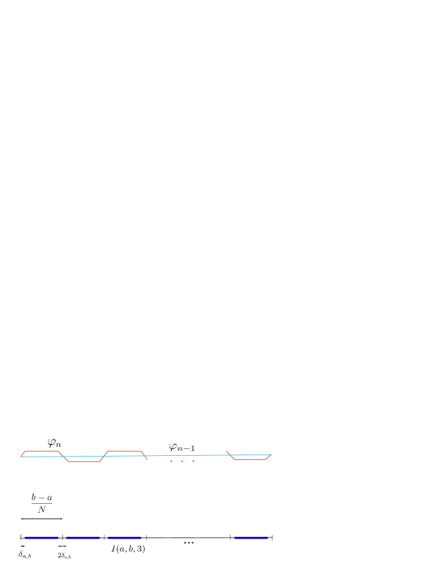
$j=1,...,N$. If we let $\delta_{a,b}=\frac{(b-a)^{2\alpha^{-1}}}{N^{2\alpha^{-1}}}$ then the intervals $I(a,b,j)$ are equally placed within $(a,b)$ with gaps $2\delta_{a,b}$ separating two consecutive such intervals, and there is a gap of length $\delta_{a,b}$ before the first and after the last such interval, see the bottom half of Figure 3. These gaps will be called later transitional intervals, due to the fact that the functions ${\phi}_{n}$ will take constant values on the intervals $I(a,b,j)$ and will change its values linearly on the transitional intervals. If $(a,b)\in{\cal I}_{n-1}$ and $x\in I(a,b,j)$ for a $j\in\{1,...,N\}$ then put

$${\phi}_{n}(x)={\phi}_{n-1}(a)+(-1)^{j+1}\frac{(b-a)^{2\alpha^{-1}}}{N^{2\alpha^{-1}}}.$$ (13)

Set

$${G}_{n}^{\prime}=\bigcup_{(a,b)\in{\cal I}_{n-1}}((a,b)\setminus\cup_{j=1}^{N}I(a,b,j)).$$ (14)

Observe that we have not defined yet the function ${\phi}_{n}$ on ${G}_{n}^{\prime}$. The system of component intervals of ${G}_{n}^{\prime}$ will be denoted by ${\cal I}_{n}^{\prime}$ and we call them transitional intervals. It will be useful later that our construction implies that if $(a,b)\in{\cal I}_{n}^{\prime}$ is a transitional interval then

$$\Big{|}\frac{{\phi}_{n}(b)-{\phi}_{n}(a)}{b-a}\Big{|}=1.$$ (15)

We define ${\phi}_{n}$ on $(a,b)\in{\cal I}_{n}^{\prime}$ so that it is linear and connects $(a,{\phi}_{n}(a))$ and $(b,{\phi}_{n}(b))$.

Set

$${G}_{n}=\bigcup_{(a,b)\in{\cal I}_{n-1}}\bigcup_{j=1}^{N}\operatorname{int}(I(a,b,j))$$ (16)

and ${\cal I}_{n}$ will denote the set of component intervals of ${G}_{n}$. We put $F_{n}=[0,1]\setminus G_{n}$. Clearly, by (10) and (12)

$$b-a<\frac{2^{\alpha/2}}{N^{n+1}}\text{ for all }(a,b)\in{\cal I}_{n}.$$ (17)

Claim 6.

We have

$$|{\phi}_{n}(x)-{\phi}_{n}(y)|\leq C_{{\phi}_{0}}(1+...+\frac{1}{2^{n}})|x-y|^{\alpha},\text{ for all }x,y\in[0,1].$$ (18)

Proof of Claim 6.

By (6) this holds for ${\phi}_{0}$. By induction, we can suppose that (18) holds for $n-1$ instead of $n$. Without limiting generality suppose that $x<y$. If $x,y\in F_{n-1}$ then ${\phi}_{n-1}(x)={\phi}_{n}(x)$ and ${\phi}_{n-1}(y)={\phi}_{n}(y)$ and our induction hypothesis implies (18). Suppose $x\in(a_{x},b_{x})\in{\cal I}_{n-1}$ and $y\in(a_{y},b_{y})\in{\cal I}_{n-1}$. (The other two cases, $x\in F_{n-1}$ , $y\in(a_{y},b_{y})\in{\cal I}_{n-1}$ and $x\in(a_{x},b_{x})\in{\cal I}_{n-1}$ and $y\in F_{n-1}$ can be treated analogously and we omit the details.)

The definition of ${\phi}_{n}$ implies that

$$|{\phi}_{n}(b_{x})-{\phi}_{n}(x)|\leq|b_{x}-x|\text{ and }|{\phi}_{n}(y)-{\phi}_{n}(a_{y})|\leq|y-a_{y}|.$$ (19)

We can suppose that $N$ is so large that

$$N^{1-\alpha}>4\text{ and }C_{{\phi}_{0}}>2.$$ (20)

By (10), $|b_{x}-a_{x}|<\frac{2}{N^{n}}$ and $|b_{y}-a_{y}|<\frac{2}{N^{n}}$. This and (20) imply

$$|b_{x}-x|^{1-\alpha}<\frac{2^{1-\alpha}}{N^{(1-\alpha)n}}<\frac{C_{{\phi}_{0}}}{2^{n+1}}\text{ and }|y-a_{y}|^{1-\alpha}<\frac{2^{1-\alpha}}{N^{(1-\alpha)n}}<\frac{C_{{\phi}_{0}}}{2^{n+1}}.$$ (21)

Using that $0<\alpha<1$ and $b_{x},a_{y}\in F_{n-1}$ we infer

$$|{\phi}_{n}(x)-{\phi}_{n}(y)|\leq|{\phi}_{n}(b_{x})-{\phi}_{n}(x)|+|{\phi}_{n-1}(b_{x})-{\phi}_{n-1}(a_{y})|+|{\phi}_{n}(y)-{\phi}_{n}(a_{y})|\leq$$

$$\frac{C_{{\phi}_{0}}}{2^{n+1}}|b_{x}-x|^{\alpha}+C_{{\phi}_{0}}(1+...+\frac{1}{2^{n-1}})|b_{x}-a_{y}|^{\alpha}+\frac{C_{{\phi}_{0}}}{2^{n+1}}|y-a_{y}|^{\alpha}<$$

$$C_{{\phi}_{0}}(1+...+\frac{1}{2^{n}})|x-y|^{\alpha}.$$

∎

If $x\in(a,b)\in{\cal I}_{0}$ then by (13)

$$|{\phi}_{1}(x)-{\phi}_{0}(x)|\leq\frac{(b-a)^{2\alpha^{-1}}}{N^{2\alpha^{-1}}}<\frac{(b-a)^{2}}{N^{2}}$$ (22)

and in general, using that for $(a^{\prime},b^{\prime})\in{\cal I}_{n-1},$ $(a^{\prime},b^{\prime})\subset(a,b)\in{\cal I}_{0}$ we have $b^{\prime}-a^{\prime}<(b-a)/N^{n-1}$ we infer

$$|{\phi}_{n}(x)-{\phi}_{n-1}(x)|\leq\frac{(b-a)^{2\alpha^{-1}}}{N^{(n-1)2\alpha^{-1}}}\cdot\frac{1}{N^{2\alpha^{-1}}}<\frac{(b-a)^{2}}{N^{2(n-1)}}\cdot\frac{1}{N^{2}}$$ (23)

for $n=2,3,...$.

3.3 Definition of the function $g_{1}$

From (23) it follows that ${\phi}_{n}(x)$ converges uniformly to a continuous function $g_{1}(x)$.

We infer from (18) that

$$|g_{1}(x)-g_{1}(y)|\leq 2C_{{\phi}_{0}}|x-y|^{\alpha}\text{ for all }x,y\in[0,1],$$ (24)

moreover by (23) for $x\in(a,b)\in{\cal I}_{0}$ we have

$$|g_{1}(x)-{\phi}_{1}(x)|\leq\frac{(b-a)^{2}}{N^{2}}\Big{(}\frac{1}{N^{2}}+\frac{1}{N^{4}}+...\Big{)}<\frac{(b-a)^{2}}{N^{2}}\cdot\frac{2}{N^{2}}.$$ (25)

From (13), (22) and (23) we also obtain for $x\in(a,b)\in{\cal I}_{0}$

$$|g_{1}(x)-{\phi}_{0}(x)|<\frac{(b-a)^{2\alpha^{-1}}}{N^{2\alpha^{-1}}}\Big{(}1+\frac{1}{N^{2}}+...\Big{)}<\frac{(b-a)^{2\alpha^{-1}}}{N^{2\alpha^{-1}}}2^{\alpha^{-1}}$$

References

- [1] O. Angel, R. Balka, A. Máthé and Y. Peres, Restrictions of Hölder continuous functions, Preprint: http://arxiv.org/abs/1504.04789.
- [2] Z. Buczolich, Monotone and convex restrictions of continuous functions, submitted, Preprint: http://arxiv.org/abs/1607.03279.
- [3] K.J. Falconer, Fractal Geometry, John Wiley & Sons, Second Edition, (2003).
- [4] J-P. Kahane, Y. Katznelson, Restrictions of continuous functions, Israel J. Math. 174 (2009), 269-284.
- [5] J-P. Kahane, Y. Katznelson, Sur un théorème de Paul Malliavin. J. Funct. Anal. 255 (2008), no. 9, 2533-2544.
- [6] A. Máthé, Measurable functions are of bounded variation on a set of Hausdorff dimension , Bull. London Math. Soc., 45 (2013), 580–594.
- [7] P. Mattila, Geometry of Sets and Measures in Euclidean Spaces, Cambridge University Press, (1995).