Particle system algorithm and chaos propagation related to non-conservative McKean type stochastic differential equations.

Abstract

We discuss numerical aspects related to a new class of nonlinear Stochastic Differential Equations in the sense of McKean, which are supposed to represent non conservative nonlinear Partial Differential equations (PDEs). We propose an original interacting particle system for which we discuss the propagation of chaos. We consider a time-discretized approximation of this particle system to which we associate a random function which is proved to converge to a solution of a regularized version of a nonlinear PDE.

Key words and phrases: Chaos propagation; Nonlinear Partial Differential Equations; McKean type Nonlinear Stochastic Differential Equations; Particle systems; Probabilistic representation of PDEs.

2010 AMS-classification: 65C05; 65C35; 68U20; 60H10; 60H30; 60J60; 58J35

1 Introduction

Stochastic differential equations of various types are very useful to investigate nonlinear partial differential equations (PDEs) at the theoretical and numerical level. From a theoretical point of view, they constitute probabilistic tools to study the analytic properties of the equation. Moreover they provide a microscopic interpretation of physical phenomena macroscopically drawn by a nonlinear PDE. From a numerical point of view, such representations allow for extended Monte Carlo type methods, which are potentially less sensitive to the dimension of the state space.
Let us consider $d,p\in\mathbb{N}^{\star}$. Let $\Phi:[0,T]\times\mathbb{R}^{d}\times\mathbb{R}\rightarrow\mathbb{R}^{d\times p}$, $g:[0,T]\times\mathbb{R}^{d}\times\mathbb{R}\rightarrow\mathbb{R}^{d}$, $\Lambda:[0,T]\times\mathbb{R}^{d}\times\mathbb{R}\rightarrow\mathbb{R}$, be Borel bounded functions, $K:\mathbb{R}^{d}\rightarrow\mathbb{R}$ be a smooth mollifier in $\mathbb{R}^{d}$ and $\zeta_{0}$ be a probability on $\mathbb{R}^{d}$. When it is absolutely continuous $v_{0}$ will denote its density so that $\zeta_{0}(dx)=v_{0}(x)dx$. The main motivation of this work is the simulation of solutions to PDEs of the form

$$\left\{\begin{array}[]{l}\partial_{t}v=\sum_{i,j=1}^{d}\partial_{ij}^{2}\big{(}(\Phi\Phi^{t})_{i,j}(t,x,v)v\big{)}-div\big{(}g(t,x,v)v\big{)}+\Lambda(t,x,v)v\\ v(0,dx)=v_{0}(dx),\end{array}\right.$$ (1.1)

through probabilistic numerical methods. Examples of nonlinear and nonconservative PDEs that are of that form arise in hydrodynamics and biological modeling. For instance one model related to underground water flows is known in the literature as the Richards equation

$$\left\{\begin{array}[]{l}\partial_{t}v=\Delta(\beta(v))+div\big{(}\alpha(v)\big{)}+\phi(x)\\ v(0,\cdot)=v_{0}\ ,\end{array}\right.$$ (1.2)

where $\beta:\mathbb{R}\longrightarrow\mathbb{R},\ \alpha:\mathbb{R}\longrightarrow\mathbb{R}^{d}$ and $\phi:\mathbb{R}^{d}\longrightarrow\mathbb{R}$. Another example concerns biological mechanisms as migration of biologial species or the evolution of a tumor growth. Such equations can be schematically written as

$$\left\{\begin{array}[]{l}\partial_{t}v=\Delta\beta(v)+f(v)\\ v(0,\cdot)=v_{0}\ ,\end{array}\right.$$ (1.3)

where $\beta:\mathbb{R}\longrightarrow\mathbb{R}$ is bounded, monotone and $f:\mathbb{R}\rightarrow\mathbb{R}$. This family of PDEs is sometimes called Porous Media type Equation with proliferation, due to the presence of the term $f$ that characterizes a proliferation phenomena and the term $\Delta\beta(v)$ delineates a porous media effect. In particular, for $\beta(v)=v^{2}$ and $f(v)=v(1-v)$, this type of equation appears in the modeling of tumors.
The present paper focuses on numerical aspects of a specific forward probabilistic representation initiated in [20], relying on nonlinear SDEs in the sense of McKean [21]. In [20], we have introduced and studied a generalized regularized McKean type nonlinear stochastic differential equation (NLSDE) of the form

$$\left\{\begin{array}[]{l}Y_{t}=Y_{0}+\int_{0}^{t}\Phi(s,Y_{s},u(s,Y_{s}))dW_{s}+\int_{0}^{t}g(s,Y_{s},u(s,Y_{s}))ds\ ,\quad\textrm{with}\quad Y_{0}\sim\zeta_{0}\ ,\\ u(t,y)=\mathbb{E}[K(y-Y_{t})\,\exp\left\{\int_{0}^{t}\Lambda\big{(}s,Y_{s},u(s,Y_{s})\big{)}ds\right\}]\ ,\quad\textrm{for any}\ t\in[0,T]\ ,\end{array}\right.$$ (1.4)

where the solution is the couple process-function $(Y,u)$. The novelty with respect to classical McKean type equations consists in the form of the second equation, where, for each $t>0$, in the classical case ($\Lambda=0$) $u(t,\cdot)$ was explicitely given by the marginal law of $Y_{t}$. The present paper aims at proposing and implementing a stochastic particle algorithm to approximate (1.4) and investigating carefully its convergence properties.
(1.4) is the probabilistic representation of the partial integro-differential equation (PIDE)

$$\left\{\begin{array}[]{l}\partial_{t}\bar{v}=\frac{1}{2}\displaystyle{\sum_{i,j=1}^{d}}\partial_{ij}^{2}\left((\Phi\Phi^{t})_{i,j}(t,x,K\ast\bar{v})\bar{v}\right)-div\left(g(t,x,K\ast\bar{v})\bar{v}\right)+\Lambda(t,x,K\ast\bar{v})\bar{v},\\ \bar{v}(0,x)=v_{0}\ ,\end{array}\right.$$ (1.5)

in the sense that, given a solution $(Y,u)$ of (1.4), there is a solution $\bar{v}$ of (1.5) in the sense of distributions, such that $u=K\ast\bar{v}:=\int_{\mathbb{R}^{d}}K(\cdot-y)\bar{v}(y)dy$. This follows, for instance, by a simple application of Itô’s formula, as explained in Theorems 6.1 and 6.2, Section 6 in [20]. Ideally our interest is devoted to (1.4) when the smoothing kernel $K$ reduces to a Dirac measure at zero. To reach that scope, one would need to replace in previous equation $K$ into $K_{\varepsilon},$ where $K_{\varepsilon}$ converges to the Dirac measure and to analyze the convergence of the corresponding solutions. However, such a theoretical analysis is out of the scope of this paper, but it will be investigated numerically via simulations reported at the end.

In fact, in the literature appear several probabilistic representations, with the objective of simulating numerically the corresponding PDE. One method which has been largely investigated for approximating solutions of time evolutionary PDEs is the method of forward-backward SDEs (FBSDEs). FBSDEs were initially developed in [23], see also [22] for a survey and [24] for a recent monograph on the subject. The idea is to express the PDE solution $v(t,\cdot)$ at time $t$ as the expectation of a functional of a so called forward diffusion process $X$, starting at time $t$. Based on that idea, many judicious numerical schemes have been proposed by [9, 14]. However, all those rely on computing recursively conditional expectation functions which is known to be a difficult task in high dimension. Besides, the FBSDE approach is blind in the sense that the forward process $X$ is not ensured to explore the most relevant space regions to approximate efficiently the solution of the FBSDE of interest. On the theoretical side, the FBSDE representation of fully nonlinear PDEs still requires complex developments and is the subject of active research (see for instance [10]). Branching diffusion processes provide alternative probabilistic representation of semi-linear PDEs, involving a specific form of non-linearity on the zero order term. This type of approach has been recently extended in [15, 16] to a more general class of non-linearities on the zero order term, with the so-called marked branching process. One of the main advantages of this approach compared to FBSDEs is that it does not involve any regression computation to calculate conditional expectations. A third class of numerical approximation schemes relies on McKean type representations. In the time continuous framework, classical McKean representations are restricted to the conservative case ($\Lambda=0$). Relevant contributions at the algorithmic level are [7, 8, 6, 4], and the survey paper [28]. In the case $\Lambda=0$ with $g=0$, but with $\Phi$ possibly discontinuous, some empirical implementations were conducted in [2, 3] in the one-dimensional and multi-dimensional case respectively, in order to predict the large time qualitative behavior of the solution of the corresponding PDE.

In the present paper we extend this type of McKean based numerical schemes to the case of non-conservative PDEs ($\Lambda\neq 0$). An interesting aspect of this approach is that it is potentially able to represent fully nonlinear PDEs, by considering a more general class of functions $\Lambda$ which may depend non-linearly not only on $u$ but on its space derivatives up to the second order. This more general setting will be focused in a future work. In the discrete-time framework, Feynman-Kac formula and various types of related particle approximation schemes were extensively analyzed in the reference books of Del Moral [12] and [13] but without considering the specific case of a time continuous system (1.4) coupled with a weighting function $\Lambda$ which depends nonlinearly on $u$.

By (3.3) we introduce an interacting particle system associated to (1.4). Indeed we replace one single McKean type stochastic differential equation with unknown process $Y$, with a system of $N$ ordinary stochastic differential equations, whose solution consists in a system of particles $\xi=(\xi^{j,N})$, replacing the law of the process $Y$ by the empirical mean law $\displaystyle{S^{N}(\xi):=\sum_{j=1}^{N}\delta_{\xi^{j,N}}}$.

In Theorem 4.2 we prove the convergence of the time-discretized particle system under Lipschitz type assumptions on the coefficients $\Phi$, $g$ and $\Lambda$, obtaining an explicit rate. The mentioned rate is based on the contribution of two effects. First, the particle approximation error between the solution $u$ of (1.4) and the approximation $u^{S^{N}(\mathbf{\xi})}$, solution of

$$u^{S^{N}(\mathbf{\xi})}_{t}(y)=\displaystyle\frac{1}{N}\sum_{j=1}^{N}K(y-\xi^{j,N}_{t})\exp\left\{\int_{0}^{t}\Lambda\big{(}s,\xi^{j,N}_{s},u^{S^{N}(\mathbf{\xi})}(s,\xi^{j,N}_{s})\big{)}ds\right\},$$ (1.6)

which is evaluated in Theorem 3.1. The second effect is the time discretization error, established in Proposition 4.1. The errors are evaluated in the $L^{p},p=2,+\infty$ mean distance, in terms of the number $N$ of particles and the time discretization step. One significant consequence of Theorem 3.1 is Corollary 3.2 which states the chaos propagation of the interacting particle system.
We emphasize that the proof of Theorem 3.1 relies on Proposition 3.3, whose formula (3.12) allows to control the particle approximation error without use of exchangeability assumptions on the particle system, see Remark 3.4.

The paper is organized as follows. After this introduction, we formulate the basic assumptions valid along the paper and recall important results proved in [20] and used in the sequel. The evaluation of the particle approximation error is discussed in Section 3. Section 4 focuses on the convergence of the time-discretized particle system. Finally in Section 5 we provide numerical simulations illustrating the performances of the interacting particle system in approximating the limit PDE (i.e. when the smoothing kernel $K$ reduces to a Dirac measure at zero), in a specific case where the solution is explicitely known.

2 Notations and assumptions

Let us consider ${\cal C}^{d}:=\mathcal{C}([0,T],\mathbb{R}^{d})$ metrized by the supremum norm $\|\cdot\|_{\infty}$, equipped with its Borel $\sigma-$ field $\mathcal{B}({\cal C}^{d})=\sigma(X_{t},t\geq 0)$ (and $\mathcal{B}_{t}({\cal C}^{d}):=\sigma(X_{u},0\leq u\leq t)$ the canonical filtration) and endowed with the topology of uniform convergence. $X$ will be the canonical process on ${\cal C}^{d}$ and $\mathcal{P}_{r}({\cal C}^{d})$ the set of Borel probability measures on ${\cal C}^{d}$ admitting a moment of order $r\geq 0$. For $r=0$, $\mathcal{P}({\cal C}^{d}):=\mathcal{P}_{0}({\cal C}^{d})$ is naturally the Polish space (with respect to the weak convergence topology) of Borel probability measures on ${\cal C}^{d}$ naturally equipped with its Borel $\sigma$-field $\mathcal{B}({\cal P}({\cal C}^{d}))$. When $d=1$, we often omit it and we simply set $\mathcal{C}:=\mathcal{C}^{1}$.
We recall that the Wasserstein distance of order $r$ and respectively the modified Wasserstein distance of order $r$ for $r\geq 1$, between $m$ and $m^{\prime}$ in $\mathcal{P}_{r}(\mathcal{C}^{d})$, denoted by $W^{r}_{T}(m,m^{\prime})$ (and resp. $\widetilde{W}^{r}_{T}(m,m^{\prime})$) are such that

$$(W^{r}_{t}(m,m^{\prime}))^{r} := \inf_{\mu\in\Pi(m,m^{\prime})}\left\{\int_{\mathcal{C}^{d}\times\mathcal{C}^{d}}\sup_{0\leq s\leq t}|X_{s}(\omega)-X_{s}(\omega^{\prime})|^{r}d\mu(\omega,\omega^{\prime})\right\},\ t\in[0,T]\ ,$$ (2.1)

$$(\widetilde{W}^{r}_{t}(m,m^{\prime}))^{r} := \inf_{\mu\in\widetilde{\Pi}(m,m^{\prime})}\left\{\int_{\mathcal{C}^{d}\times\mathcal{C}^{d}}\sup_{0\leq s\leq t}|X_{s}(\omega)-X_{s}(\omega^{\prime})|^{r}\wedge 1\;d\mu(\omega,\omega^{\prime})\right\},\ t\in[0,T]\ ,$$ (2.2)

where $\Pi(m,m^{\prime})$ (resp. $\widetilde{\Pi}(m,m^{\prime})$) denotes the set of Borel probability measures in ${\cal P}({\cal C}^{d}\times{\cal C}^{d})$ with fixed marginals $m$ and $m^{\prime}$ belonging to ${\cal P}_{r}({\cal C}^{d})$ (resp. ${\cal P}({\cal C}^{d})$ ). In this paper we will use very frequently the Wasserstein distances of order $2$. For that reason, we will simply set $W_{t}:=W^{2}_{t}$ (resp. ${\tilde{W}}_{t}:={\tilde{W}}^{2}_{t}$).
Given $N\in\mathbb{N}^{\star}$, $l\in{\cal C}^{d}$, $l^{1},\cdots,l^{N}\in{\cal C}^{d}$, a significant role in this paper will be played by the Borel measures on ${\cal C}^{d}$ given by $\delta_{l}$ and $\displaystyle{\frac{1}{N}\sum_{j=1}^{N}\delta_{l^{j}}}$.

Remark 2.1.

Given $l^{1},\cdots,l^{N},\tilde{l}^{1},\cdots,\tilde{l}^{N}\in{\cal C}^{d}$, by definition of the Wasserstein distance we have, for all $t\in[0,T]$

$$W_{t}\left(\frac{1}{N}\sum_{j=1}^{N}\delta_{l^{j}},\frac{1}{N}\sum_{j=1}^{N}\delta_{\tilde{l}^{j}}\right)\leq\frac{1}{N}\sum_{j=1}^{N}\sup_{0\leq s\leq t}|l^{j}_{s}-\tilde{l}^{j}_{s}|^{2}\ .$$

In this paper ${\cal C}_{b}({\cal C}^{d})$ denotes the space of bounded, continuous real-valued functions on ${\cal C}^{d}$, for which the supremum norm is denoted by $\|\cdot\|_{\infty}$. $\mathbb{R}^{d}$ is equipped with the scalar product $\cdot$ and $|x|$ stands for the induced Euclidean norm for $x\in\mathbb{R}^{d}$. Given two reals $a$, $b$ ($d=1$) we will denote in the sequel $a\wedge b:=\min(a,b)$ and $a\vee b:=\max(a,b)$.
$\mathcal{M}_{f}(\mathbb{R}^{d})$ is the space of finite, Borel measures on $\mathbb{R}^{d}$. $\mathcal{S}(\mathbb{R}^{d})$ is the space of Schwartz fast decreasing test functions and $\mathcal{S}^{\prime}(\mathbb{R}^{d})$ is its dual. $\mathcal{C}_{b}(\mathbb{R}^{d})$ is the space of bounded, continuous functions on $\mathbb{R}^{d}$, $\mathcal{C}^{\infty}_{0}(\mathbb{R}^{d})$ is the space of smooth functions with compact support. $\mathcal{C}^{\infty}_{b}(\mathbb{R}^{d})$ is the space of bounded and smooth functions. $\mathcal{C}_{0}(\mathbb{R}^{d})$ represents the space of continuous functions with compact support in $\mathbb{R}^{d}$. $W^{r,p}(\mathbb{R}^{d})$ is the Sobolev space of order $r\in\mathbb{N}$ in $(L^{p}(\mathbb{R}^{d}),||\cdot||_{p})$, with $1\leq p\leq\infty$.
$\mathcal{F}(\cdot):f\in\mathcal{S}(\mathbb{R}^{d})\mapsto\mathcal{F}(f)\in\mathcal{S}(\mathbb{R}^{d})$ will denote the Fourier transform on the classical Schwartz space $\mathcal{S}(\mathbb{R}^{d})$ such that for all $\xi\in\mathbb{R}^{d}$,

$$\mathcal{F}(f)(\xi)=\frac{1}{\sqrt{2\pi}}\int_{\mathbb{R}^{d}}f(x)e^{-i\xi\cdot x}dx\ .$$

We will designate in the same manner the corresponding Fourier transform on $\mathcal{S}^{\prime}(\mathbb{R}^{d})$.

For any Polish space $E$, we will designate by ${\cal B}(E)$ its Borel $\sigma$-field. It is well-known that ${\cal P}(E)$ is also a Polish space with respect to the weak convergence topology, whose Borel $\sigma$-field will be denoted by ${\cal B}({\cal P}(E))$ (see Proposition 7.20 and Proposition 7.23, Section 7.4 Chapter 7 in [5]).
Let $(\Omega,{\cal F})$ be a measured space. A map $\eta:(\Omega,{\cal F})\longrightarrow({\cal P}(E),{\cal B}({\cal P}(E)))$ will be called random probability (or random probability kernel) if it is measurable. We will indicate by ${\cal P}^{\Omega}(E)$ the space of random probabilities.

Remark 2.2.

Let $\eta:(\Omega,{\cal F})\longrightarrow({\cal P}(E),{\cal B}({\cal P}(E)))$. $\eta$ is a random probability if and only if the two following conditions hold:

• for each $\bar{\omega}\in\Omega$, $\eta_{\bar{\omega}}\in{\cal P}(E)$,

• for all Borel set $A\in{\cal B}({\cal P}(E))$, $\bar{\omega}\mapsto\eta_{\bar{\omega}}(A)$ is ${\cal F}$-measurable.

This was highlighted in Remark 3.20 in [11] (see also Proposition 7.25 in [5]).

Remark 2.3.

Given $\mathbb{R}^{d}$-valued continuous processes $Y^{1},\cdots,Y^{n}$, the application $\displaystyle{\frac{1}{N}\sum_{j=1}^{N}\delta_{Y^{j}}}$ is a random probability on ${\cal P}({\cal C}^{d})$. In fact $\delta_{Y^{j}},1\leq j\leq N$ is a random probability by Remark 2.2.

In this article, the following assumptions will be used.

Assumption 1.

1. $\Phi$ and $g$ Borel functions defined on $[0,T]\times\mathbb{R}^{d}\times\mathbb{R}$ taking values respectively in $\mathbb{R}^{d\times p}$ (space of $d\times p$ matrices) and $\mathbb{R}^{d}$ that are Lipschitz w.r.t. space variables: there exist finite positive reals $L_{\Phi}$ and $L_{g}$ such that for any $(t,y,y^{\prime},z,z^{\prime})\in[0,T]\times\mathbb{R}^{d}\times\mathbb{R}^{d}\times\mathbb{R}\times\mathbb{R}$, we have

   $$|\Phi(t,y^{\prime},z^{\prime})-\Phi(t,y,z)|\leq L_{\Phi}(|z^{\prime}-z|+|y^{\prime}-y|)\quad\textrm{and}\quad|g(t,y^{\prime},z^{\prime})-g(t,y,z)|\leq L_{g}(|z^{\prime}-z|+|y^{\prime}-y|)\ .$$

2. $\Lambda$ is a Borel real valued function defined on $[0,T]\times\mathbb{R}^{d}\times\mathbb{R}$ Lipschitz w.r.t. the space variables: there exists a finite positive real, $L_{\Lambda}$ such that for any $(t,y,y^{\prime},z,z^{\prime})\in[0,T]\times\mathbb{R}^{d}\times\mathbb{R}^{d}\times\mathbb{R}\times\mathbb{R}$, we have

   $$|\Lambda(t,y,z)-\Lambda(t,y^{\prime},z^{\prime})|\leq L_{\Lambda}(|y^{\prime}-y|+|z^{\prime}-z|)\ .$$

3. $\Lambda$ is supposed to be uniformly bounded: there exist a finite positive real $M_{\Lambda}$ such that, for any $(t,y,z)\in[0,T]\times\mathbb{R}^{d}\times\mathbb{R}$

   $$|\Lambda(t,y,z)|\leq M_{\Lambda}\ .$$

4. $K:\mathbb{R}^{d}\rightarrow\mathbb{R}_{+}$ is integrable, Lipschitz, bounded and whose integral is 1: there exist finite positive reals $M_{K}$ and $L_{K}$ such that for any $(y,y^{\prime})\in\mathbb{R}^{d}\times\mathbb{R}^{d}$

   $$|K(y)|\leq M_{K},\quad|K(y^{\prime})-K(y)|\leq L_{K}|y^{\prime}-y|\ \quad\textrm{and}\quad\int_{\mathbb{R}^{d}}K(x)dx=1\ .$$

5. $\zeta_{0}$ is a fixed Borel probability measure on $\mathbb{R}^{d}$ admitting a second order moment.

6. The functions $s\in[0,T]\mapsto\Phi(s,0,0)$ and $s\in[0,T]\mapsto g(s,0,0)$ are bounded. $m_{\Phi}$ (resp. $m_{g}$) will denote the supremum $\sup_{s\in[0,T]}|\Phi(s,0,0)|$ (resp. $\sup_{s\in[0,T]}|g(s,0,0)|$).

Given a finite signed Borel measure $\gamma$ on $\mathbb{R}^{d}$, $K*\gamma$ will denote the convolution function $x\mapsto\gamma(K(x-\cdot))$. In particular if $\gamma$ is absolutely continuous with density ${\dot{\gamma}}$, then $(K*\gamma)(x)=\int_{\mathbb{R}^{d}}K(x-y)\dot{\gamma}(y)dy$.

To simplify we introduce the following notations.

• $V\,:[0,T]\times{\mathcal{C}}^{d}\times\mathcal{C}\rightarrow\mathbb{R}$ defined for any pair of functions $y\in\mathcal{C}^{d}$ and $z\in\mathcal{C}$, by

  $$V_{t}(y,z):=\exp\left(\int_{0}^{t}\Lambda(s,y_{s},z_{s})ds\right)\quad\textrm{for any}\ t\in[0,T]\ .$$ (2.3)

• The real valued process $Z$ such that $Z_{s}=u(s,Y_{s})$, for any $s\in[0,T]$, will often be denoted by $u(Y)$.

With these new notations, the second equation in (1.4) can be rewritten as

$$\nu_{t}(\varphi)=\mathbb{E}[(\check{K}\ast\varphi)(Y_{t})V_{t}(Y,u(Y))]\ ,\quad\textrm{for any}\ \varphi\in\mathcal{C}_{b}(\mathbb{R}^{d},\mathbb{R})\ ,\\$$ (2.4)

where $u(t,\cdot)=\frac{d\nu_{t}}{dx}$ and $\check{K}(x):=K(-x)$.

Remark 2.4.

Under Assumption 1. 3.(b), $\Lambda$ is bounded. Consequently

$$0\leq V_{t}(y,z)\leq e^{tM_{\Lambda}}\ ,\quad\textrm{for any}\ (t,y,z)\in[0,T]\times\mathbb{R}^{d}\times\mathbb{R}\ .$$ (2.5)

Under Assumption 1. 2. $\Lambda$ is Lipschitz. Then $V$ inherits in some sense this property. Indeed, observe that for any $(a,b)\in\mathbb{R}^{2}$,

$$e^{b}-e^{a}=(b-a)\int_{0}^{1}e^{\alpha b+(1-\alpha)a}d\alpha\leq e^{\sup(a,b)}|b-a|\ .$$ (2.6)

Then for any continuous functions $y,\,y^{\prime}\in\mathcal{C}^{d}=\mathcal{C}([0,T],\mathbb{R}^{d})$, and $z,\,z^{\prime}\in\mathcal{C}([0,T],\mathbb{R})$, taking $a=\int_{0}^{t}\Lambda(s,y_{s},z_{s})ds$ and $b=\int_{0}^{t}\Lambda(s,y^{\prime}_{s},z^{\prime}_{s})ds$ in the above equality yields

$$|V_{t}(y^{\prime},z^{\prime})-V_{t}(y,z)| \leq e^{tM_{\Lambda}}\int_{0}^{t}\left|\Lambda(s,y^{\prime}_{s},z^{\prime}_{s})-\Lambda(s,y_{s},z_{s})\right|ds$$ (2.7)

$$\leq e^{tM_{\Lambda}}L_{\Lambda}\,\int_{0}^{t}\left(|y^{\prime}_{s}-y_{s}|+|z^{\prime}_{s}-z_{s}|\right)ds\ .$$

In Section 4, Assumption 1. will be replaced by what follows.

Assumption 2.

All items of Assumption 1. are in force excepted 1. and 2. which are replaced by the following.

1. There exist positive reals $L_{\Phi}$, $L_{g}$ such that, for any $(t,t^{\prime},y,y^{\prime},z,z^{\prime})\in[0,T]^{2}\times(\mathbb{R}^{d})^{2}\times\mathbb{R}^{2}$,

   $$|\Phi(t,y,z)-\Phi(t^{\prime},y^{\prime},z^{\prime})|\leq L_{\Phi}\,(|t-t^{\prime}|^{\frac{1}{2}}+|y-y^{\prime}|+|z-z^{\prime}|),$$

   $$|g(t,y,z)-g(t^{\prime},y^{\prime},z^{\prime})|\leq L_{g}\,(|t-t^{\prime}|^{\frac{1}{2}}+|y-y^{\prime}|+|z-z^{\prime}|).$$

2. There exists a positive real $L_{\Lambda}$ such that, for any $(t,t^{\prime},y,y^{\prime},z,z^{\prime})\in[0,T]^{2}\times(\mathbb{R}^{d})^{2}\times\mathbb{R}^{2}$,

   $$|\Lambda(t,y,z)-\Lambda(t^{\prime},y^{\prime},z^{\prime})|\leq L_{\Lambda}\,(|t-t^{\prime}|^{\frac{1}{2}}+|y-y^{\prime}|+|z-z^{\prime}|).$$

We end this section by recalling important results established in our companion paper [20], for which Assumption 1. is supposed to be satisfied. Let us first remark that the second equation of (1.4) can be rewritten as

$$u^{m}(t,y)=\int_{{\cal C}^{d}}K(y-\omega_{t})\exp\Big{\{}\int_{0}^{t}\Lambda(s,\omega_{s},u^{m}(s,\omega_{s}))\Big{\}}dm(\omega),\;(t,x)\in[0,T]\times\mathbb{R}^{d},$$ (2.8)

with $m=m_{Y}$ being the law of the process $Y$ on the canonical space ${\cal C}^{d}$.
Indeed for every $m\in{\cal P}({\cal C}^{d})$, Theorem 3.1 of [20] shows that equation (2.8) is well-posed and so it properly defines a function $u^{m}$. The lemma below, established in Proposition 3.3 of [20], states stability results on the function $(m,t,y)\mapsto u^{m}(t,y)$.

Proposition 2.5.

We assume the validity of items $2.$, $3$ and $4.$ of Assumption 1.
The following assertions hold.

1. For any couple of probabilities $(m,m^{\prime})\in\mathcal{P}_{2}(\mathcal{C}^{d})\times\mathcal{P}_{2}(\mathcal{C}^{d})$, for all $(t,y,y^{\prime})\in[0,T]\times{\cal C}^{d}\times{\cal C}^{d}$, we have

   $$|u^{m}\big{(}t,y\big{)}-u^{m^{\prime}}\big{(}t,y^{\prime}\big{)}|^{2}\leq C_{K,\Lambda}(t)\left[|y-y^{\prime}|^{2}+|W_{t}(m,m^{\prime})|^{2}\right]\ ,$$ (2.9)

   where $C_{K,\Lambda}(t):=2C^{\prime}_{K,\Lambda}(t)(t+2)(1+e^{2tC^{\prime}_{K,\Lambda}(t)})$ with $C^{\prime}_{K,\Lambda}(t)=2e^{2tM_{\Lambda}}(L^{2}_{K}+2M^{2}_{K}L^{2}_{\Lambda}t)$. In particular the functions $C_{K,\Lambda}$ only depend on $M_{K},L_{K},M_{\Lambda},L_{\Lambda}$ and $t$ and is increasing with $t$.

2. For any $(m,m^{\prime})\in{\cal P}(C^{d})\times{\cal P}(C^{d})$, for all $(t,y,y^{\prime})\in[0,T]\times{\cal C}^{d}\times{\cal C}^{d}$, we have

   $$|u^{m}\big{(}t,y\big{)}-u^{m^{\prime}}\big{(}t,y^{\prime}\big{)}|^{2}\leq\mathfrak{C}_{K,\Lambda}(t)\left[|y-y^{\prime}|^{2}+|\widetilde{W}_{t}(m,m^{\prime})|^{2}\right]\ ,$$ (2.10)

   where $\mathfrak{C}_{K,\Lambda}(t):=2e^{2tM_{\Lambda}}(\max(L_{K},2M_{K})^{2}+2M_{K}^{2}\max(L_{\Lambda},2M_{\Lambda})^{2}t)$.

3. The function $(m,t,x)\mapsto u^{m}(t,x)$ is continuous on ${\cal P}({\cal C}^{d})\times[0,T]\times\mathbb{R}^{d},$ where ${\cal P}({\cal C}^{d})$ is endowed with the topology of weak convergence.

4. Suppose that $K\in W^{1,2}(\mathbb{R}^{d})$. Then for any $(m,m^{\prime})\in\mathcal{P}_{2}(\mathcal{C}^{d})\times\mathcal{P}_{2}(\mathcal{C}^{d})$, $t\in[0,T]$

   $$\|u^{m}(t,\cdot)-u^{m^{\prime}}(t,\cdot)\|_{2}^{2}\leq\tilde{C}_{K,\Lambda}(t)(1+2tC_{K,\Lambda}(t))|W_{t}(m,m^{\prime})|^{2}\ ,$$ (2.11)

   where $C_{K,\Lambda}(t):=2C^{\prime}_{K,\Lambda}(t)(t+2)(1+e^{2tC^{\prime}_{K,\Lambda}(t)})$ with $C^{\prime}_{K,\Lambda}(t)=2e^{2tM_{\Lambda}}(L^{2}_{K}+2M^{2}_{K}L^{2}_{\Lambda}t)$ and $\tilde{C}_{K,\Lambda}(t):=2e^{2tM_{\Lambda}}(2M_{K}L_{\Lambda}^{2}t(t+1)+\|\nabla K\|_{2}^{2})$, $\|\cdot\|_{2}$ being the standard $L^{2}(\mathbb{R}^{d})$ or $L^{2}(\mathbb{R}^{d},\mathbb{R}^{d})$-norms.
   In particular the functions $t\mapsto C^{\prime}_{K,\Lambda}(t)$ and $t\mapsto C_{K,\Lambda}(t)$ only depend on $M_{K},L_{K},M_{\Lambda},L_{\Lambda}$ and are increasing with respect to $t$.

5. Suppose that ${\cal F}(K)\in L^{1}(\mathbb{R}^{d})$. Then there exists a constant $\bar{C}_{K,\Lambda}(t)>0$ (depending only on $t,M_{\Lambda},L_{\Lambda},\|{\cal F}(K)\|_{1}$) such that for any random probability $\eta:(\Omega,{\cal F})\longrightarrow({\cal P}_{2}({\cal C}^{d}),{\cal B}({\cal P}({\cal C}^{d})))$, for all $(t,m)\in[0,T]\times{\cal P}({\cal C}^{d})$

   $$\mathbb{E}{[\|u^{\eta}(t,\cdot)-u^{m}(t,\cdot)\|_{\infty}^{2}]} \leq \bar{C}_{K,\Lambda}(t)\sup_{\underset{\|\varphi\|_{\infty}\leq 1}{\varphi\in{\cal C}_{b}({\cal C}^{d})}}\mathbb{E}{[|\langle\eta-m,\varphi\rangle|^{2}]}\ ,$$ (2.12)

   where we recall that ${\cal P}({\cal C}^{d})$ is endowed with the topology of weak convergence. We remark that the expectation in both sides of (2.12) is taken w.r.t. the randomness of the random probability $\eta$.

Remark 2.6.

The map $\displaystyle{d_{2}^{\Omega}:(\nu,\mu)\mapsto\sqrt{\sup_{\underset{\|\varphi\|_{\infty}\leq 1}{\varphi\in{\cal C}_{b}({\cal C}^{d})}}\mathbb{E}[|\langle\nu-\mu,\varphi\rangle|^{2}]}}$ defines a (homogeneous) distance on ${\cal P}^{\Omega}({\cal C}^{d})$.

The lemma below was proved in Lemma 7.1 in [20].

Lemma 2.7.

Let $r:\,[0,T]\mapsto[0,T]$ be a non-decreasing function such that $r(s)\leq s$ for any $s\in[0,T]$ and $Y_{0}$ be a random variable admitting $\zeta_{0}$ as law.
Let ${\cal U}:(t,y)\in[0,T]\times{\cal C}^{d}\rightarrow\mathbb{R}$ (respectively ${\cal U}^{\prime}:(t,y)\in[0,T]\times{\cal C}^{d}\rightarrow\mathbb{R}$), be a given Borel function such that for all $t\in[0,T]$, there is a Borel map ${\cal U}_{t}:{\cal C}([0,t],\mathbb{R}^{d})\rightarrow\mathbb{R}$ (resp. ${\cal U}^{{}^{\prime}}_{t}:{\cal C}([0,t],\mathbb{R}^{d})\rightarrow\mathbb{R}$) such that ${\cal U}(t,\cdot)={\cal U}_{t}(\cdot)$ (resp. ${\cal U}^{\prime}(t,\cdot)={\cal U}^{\prime}_{t}(\cdot)$).

Then the following two assertions hold.

1. Consider $Y$ (resp. $Y^{\prime}$) a solution of the following SDE for $v={\cal U}$ (resp. $v={\cal U}^{\prime}$):

   $$\begin{array}[]{l}Y_{t}=Y_{0}+\int_{0}^{t}\Phi(r(s),Y_{r(s)},v(r(s),Y_{\cdot\wedge r(s)}))dW_{s}+\int_{0}^{t}g(r(s),Y_{r(s)},v(r(s),Y_{\cdot\wedge r(s)}))ds\ ,\quad\textrm{for any}\ t\in[0,T]\ ,\end{array}$$ (2.13)

   where, we emphasize that for all $\theta\in[0,T]$, $Z_{\cdot\wedge\theta}:=\{Z_{u},0\leq u\leq\theta\}\in{\cal C}([0,\theta],\mathbb{R}^{d})$ for any continuous process $Z$. For any $a\in[0,T]$, we have

   $$\mathbb{E}[\sup_{t\leq a}|Y^{\prime}_{t}-Y_{t}|^{2}]\leq C_{\Phi,g}(T)\mathbb{E}\left[\int_{0}^{a}|{\cal U}(r(t),Y_{\cdot\wedge r(t)})-{\cal U}^{\prime}(r(t),Y^{\prime}_{\cdot\wedge r(t)})|^{2}dt\right]\ ,$$ (2.14)

   where $C_{\Phi,g}(T)=12(4L^{2}_{\Phi}+TL^{2}_{g})e^{12T(4L^{2}_{\Phi}+TL^{2}_{g})}$.

2. Suppose moreover that $\Phi$ and $g$ are $\frac{1}{2}$-Hölder w.r.t. the time and Lipschitz w.r.t. the space variables i.e. there exist some positive constants $L_{\Phi}$ and $L_{g}$ such that for any $(t,t^{\prime},y,^{\prime}y^{\prime},z,z^{\prime})\in[0,T]^{2}\times\mathbb{R}^{2d}\times\mathbb{R}^{2}$

   $$\left\{\begin{array}[]{l}|\Phi(t,y,z)-\Phi(t^{\prime},y^{\prime},z^{\prime})|\leq L_{\Phi}(|t-t^{\prime}|^{\frac{1}{2}}+|y-y^{\prime}|+|z-z^{\prime}|)\\ |g(t,y,z)-g(t^{\prime},y^{\prime},z^{\prime})|\leq L_{g}(|t-t^{\prime}|^{\frac{1}{2}}+|y-y^{\prime}|+|z-z^{\prime}|)\ .\end{array}\right.$$ (2.15)

   Let $r_{1},r_{2}:\,[0,T]\mapsto[0,T]$ being two non-decreasing functions verifying $r_{1}(s)\leq s$ and $r_{2}(s)\leq s$ for any $s\in[0,T]$. Let $Y$ (resp. $Y^{\prime}$) be a solution of (2.13) for $v={\cal U}$ and $r=r_{1}$ (resp. $v={\cal U}^{\prime}$ and $r=r_{2}$). Then for any $a\in[0,T]$, the following inequality holds:

   $$\mathbb{E}[\sup_{t\leq a}|Y^{\prime}_{t}-Y_{t}|^{2}] \leq C_{\Phi,g}(T)\left(\|r_{1}-r_{2}\|_{L^{1}([0,T])}+\int_{0}^{a}\mathbb{E}[|Y^{\prime}_{r_{1}(t)}-Y^{\prime}_{r_{2}(t)}|^{2}]dt\right.$$ (2.16)

   $$\left.+\mathbb{E}\left[\int_{0}^{a}|{\cal U}(r_{1}(t),Y_{\cdot\wedge r_{1}(t)})-{\cal U}^{\prime}(r_{2}(t),Y^{\prime}_{\cdot\wedge r_{2}(t)})|^{2}dt\textasciiacute\right]\right)\ ,$$

The theorem below was the object of Theorem 3.9 in [20].

Theorem 2.8.

Under Assumption 1, the McKean type SDE (1.4) admits strong existence and pathwise uniqueness.

For a precise formulation of the notion of existence and uniqueness for the McKean type equation (1.4) we refer to Definition 2.6 of [20].

We finally recall an important non-anticipating property of the map $(m,t,x)\mapsto u^{m}(t,x)$, stated in [20].

Definition 2.9.

Let us fix $t\in[0,T]$. Given a non-negative Borel measure $m$ on $(\mathcal{C}^{d},{\cal B}({\cal C}^{d}))$. From now on, $m_{t}$ will denote the (unique) induced measure on $(\mathcal{C}_{t}^{d},{\cal B}({\cal C}^{d}_{t}))$ (with $\mathcal{C}_{t}^{d}:=\mathcal{C}([0,t],\mathbb{R}^{d})$) defined by

$$\int_{\mathcal{C}_{t}^{d}}F(\phi)m_{t}(d\phi)=\int_{\mathcal{C}^{d}}F(\phi_{|_{[0,t]}})m(d\phi),$$

where $F:\mathcal{C}_{t}^{d}\longrightarrow\mathbb{R}$ is bounded and continuous.

Remark 2.10.

Let $t\in[0,T],m=\delta_{\xi}\;,\xi\in\mathcal{C}^{d}$. The induced measure $m_{t}$, on ${\cal C}_{t}^{d}$, is $\delta_{(\xi_{r}|0\leq r\leq t)}$.

For each $t\in[0,T]$, the same construction as the one carried on in Theorem 3.1 in [20] allows us to define the unique solution to

$$\begin{array}[]{l}u^{m_{t}}(s,y)=\int_{\mathcal{C}_{t}^{d}}K(y-X_{s}(\omega))\exp\left(\int_{0}^{s}\Lambda(r,X_{r}(\omega),u^{m_{t}}(r,X_{r}(\omega)))dr\right)m_{t}(d\omega)\quad\ \forall s\in[0,t]\ .\end{array}$$ (2.17)

The proposition and corollary below were the object of Proposition 3.7 and Corollary 3.8 in [20].

Proposition 2.11.

Under Assumption 1, we have

$$\forall(s,y)\in[0,t]\times\mathbb{R}^{d},\;u^{m}(s,y)=u^{m_{t}}(s,y).$$

Corollary 2.12.

Let $N\in\mathbb{N}$, $\xi^{1},\cdots,\xi^{i},\cdots,\xi^{N}$ be $(\mathcal{G}_{t})$-adapted continuous processes, where $\mathcal{G}$ is a filtration (defined on some probability space) fulfilling the usual conditions. Let $m(d\omega)=\frac{1}{N}\sum_{i=1}^{N}\delta_{\xi^{i}}(d\omega)$. Then, $(u^{m}(t,y))$ is a $(\mathcal{G}_{t})$-adapted random field, i.e. for any $(t,y)\in[0,T]\times\mathbb{R}^{d}$, the process is $(\mathcal{G}_{t})$-adapted.

3 Particle systems approximation and propagation of chaos

In this section, we introduce an interacting particle system $\xi=(\xi^{i,N})_{i=1,\cdots,N}$ whose empirical law will be shown to converge to the law of the solution $Y$ of the McKean type equation (1.4). A consequence of the so called propagation of chaos which describes the asymptotic independence of the components of $\xi$ when the size $N$ of the particle system goes to $\infty$. That property was introduced in [21] and further developed and popularized by [27]. The convergence of $(\xi^{i,N})_{i=1,\cdots,N}$ induces a natural approximation of $u$, solution of (1.4).
We suppose here the validity of Assumption 1. Let $(\Omega,\mathcal{F},\mathbb{P})$ be a fixed probability space, and $(W^{i})_{i=1,\cdots,N}$ be a sequence of independent $\mathbb{R}^{p}$-valued Brownian motions. Let $(Y_{0}^{i})_{i=1,\cdots,N}$ be i.i.d. r.v. according to $\zeta_{0}$. We consider $\mathbf{Y}:=(Y^{i})_{i=1,\cdots,N}$ the sequence of processes such that $(Y^{i},u^{m^{i}})$ are solutions to

$$\left\{\begin{array}[]{l}Y^{i}_{t}=Y_{0}^{i}+\int_{0}^{t}\Phi(s,Y^{i}_{s},u^{m^{i}}_{s}(Y^{i}_{s}))dW^{i}_{s}+\int_{0}^{t}g(s,Y^{i}_{s},u^{m^{i}}_{s}(Y^{i}_{s}))ds\\ u^{m^{i}}_{t}(y)={\displaystyle\mathbb{E}\left[K(y-Y^{i}_{t})V_{t}\big{(}Y^{i},u^{m^{i}}(Y^{i})\big{)}\right]}\ ,\quad\textrm{with}\ m^{i}:=\mathcal{L}(Y^{i})\ ,\end{array}\right.$$ (3.1)

recalling that $V_{t}\big{(}Y^{i},u^{m^{i}}(Y^{i})\big{)}=\exp\big{(}\int_{0}^{t}\Lambda_{s}(Y^{i}_{s},u^{m^{i}}_{s}(Y^{i}_{s}))ds\big{)}$. The existence and uniqueness of the solution of each equation is ensured by Theorem 2.8. We recall that the map $(m,t,y)\mapsto u^{m}(t,y)$ fulfills the regularity properties given at the second and third item of Proposition 2.5 .

Obviously the processes $(Y^{i})_{i=1,\cdots,N}$ are independent. They are also identically distributed since Theorem 2.8 also states uniqueness in law.
So we can define $m^{0}:=m^{i}$ the common distribution of the processes $Y^{i},i=1,\cdots,N$, which is of course the law of the process $Y$, such that $(Y,u)$ is a solution of (1.4).
From now on, ${\mathcal{C}}^{dN}$ will denote $({\mathcal{C}}^{d})^{N}$, which is obviously isomorphic to ${\cal C}([0,T],\mathbb{R}^{dN})$. For every $\bar{\xi}\in{\mathcal{C}}^{dN}$ we will denote

$$S^{N}(\mathbf{\bar{\xi}}):=\frac{1}{N}\sum_{i=1}^{N}\delta_{\bar{\xi}^{i,N}}.$$ (3.2)

The function $(t,x)\mapsto u^{S^{N}(\mathbf{\bar{\xi}})}_{t}(x)$ is obtained by composition of $m\mapsto u^{m}_{t}(x)$ (defined in (2.8)) with $m=S^{N}(\mathbf{\bar{\xi}})$.

Now let us introduce the system of equations

$$\left\{\begin{array}[]{l}\xi^{i,N}_{t}=\xi^{i,N}_{0}+\int_{0}^{t}\Phi(s,\xi^{i,N}_{s},u^{S^{N}(\mathbf{\xi})}_{s}(\xi^{i,N}_{s}))dW^{i}_{s}+\int_{0}^{t}g(s,\xi^{i,N}_{s},u^{S^{N}(\mathbf{\xi})}_{s}(\xi^{i,N}_{s}))ds\\ \xi^{i,N}_{0}=Y^{i}_{0}\\ u^{S^{N}(\mathbf{\xi})}_{t}(y)={\displaystyle\frac{1}{N}\sum_{j=1}^{N}K(y-\xi^{j,N}_{t})V_{t}\big{(}\xi^{j,N},u^{S^{N}(\mathbf{\xi})}(\xi^{j,N})\big{)}}\ .\end{array}\right.$$ (3.3)

Conformally with (3.2), we consider the empirical (random) measure $\displaystyle{S^{N}(\mathbf{Y})=\frac{1}{N}\sum_{i=1}^{N}\delta_{Y^{i}}}$ related to ${\bf Y}:=(Y^{i})_{i=1,\cdots,N},$ where we recall that for each $i\in\{1,\cdots,N\}$, $Y^{i}$ is solution of (3.1). We observe that by Remark 2.3, $S^{N}(\mathbf{\xi})$ and $S^{N}(\mathbf{Y})$ are measurable maps from $(\Omega,{\cal F})$ to $({\cal P}({\cal C}^{d}),{\cal B}({\cal P}({\cal C}^{d})))$; moreover $S^{N}(\xi),S^{N}({\bf{Y}})\in{\cal P}_{2}({\cal C}^{d})$ $\mathbb{P}$-a.s. A solution ${\bf{\xi}}:=(\xi^{i,N})_{i=1,\cdots,N}$ of (3.3) is called interacting particle system.

The first line of (3.3) is in fact a path-dependent stochastic differential equation. We claim that its coefficients are measurable. Indeed, the map $(t,\bar{\xi})\mapsto(S^{N}(\bar{\xi}),t,\bar{\xi}_{t}^{i},)$ being continuous from $([0,T]\times{\cal C}^{dN},{\cal B}([0,T])\otimes{\cal B}({\cal C}^{dN}))$ to $({\cal P}({\cal C}^{d})\times[0,T]\times\mathbb{R}^{d},{\cal B}({\cal P}({\cal C}^{d}))\otimes{\cal B}([0,T])\otimes{\cal B}(\mathbb{R}^{d}))$ for all $i\in\{1,\cdots,N\}$, by composition with the continuous map $(m,t,y)\mapsto u^{m}(t,y)$ (see Proposition 2.5 3.) we deduce the continuity of $(t,\bar{\xi})\mapsto(u_{t}^{S^{N}(\bar{\xi})}(\bar{\xi}^{i}_{t}))_{i=1,\cdots,N}$, and so the measurability from $([0,T]\times{\cal C}^{dN},{\cal B}([0,T])\otimes{\cal B}({\cal C}^{dN}))$ to $(\mathbb{R},{\cal B}(\mathbb{R}))$.
In the sequel, for simplicity we set $\bar{\xi}_{r\leq s}:=(\bar{\xi}^{i}_{r\leq s})_{1\leq i\leq N}$. We remark that, by Proposition 2.11 and Remark 2.10, we have

$$\left(u^{S^{N}(\bar{\xi})}_{s}(\bar{\xi}^{i}_{s})\right)_{i=1,\cdots N}=\left(u^{S^{N}(\mathbf{\bar{\xi}_{r\leq s}})}_{s}(\bar{\xi}^{i}_{s})\right)_{i=1,\cdots N},$$ (3.4)

for any $s\in[0,T],\;\bar{\xi}\in{\mathcal{C}}^{dN}$ and so stochastic integrands of (3.3) are adapted (so progressively measurable being continuous in time) and so the corresponding Itô integral makes sense. We discuss below the well-posedness of (3.3).
The fact that (3.3) has a unique (strong) solution $(\xi^{i,N})_{i=1,\cdots N}$ holds true because of the following arguments.

1. $\Phi$ and $g$ are Lipschitz. Moreover the map $\mathbf{\bar{\xi}}_{r\leq s}\mapsto\left(u^{S^{N}(\mathbf{\bar{\xi}_{r\leq s}})}_{s}(\bar{\xi}^{i}_{s})\right)_{i=1,\cdots,N}$ is Lipschitz.
   Indeed, for given $(\xi_{r\leq s},\eta_{r\leq s})\in{\cal C}^{dN}\times{\cal C}^{dN}$, $s\in[0,T]$, by using successively inequality (2.9) of Proposition 2.5 and Remark 2.1, for all $i\in\{1,\cdots,N\}$ we have

   $$|u_{s}^{S^{N}(\xi_{r\leq s})}(\xi^{i}_{t})-u_{s}^{S^{N}(\eta_{r\leq s})}(\eta^{i}_{t})| \leq \sqrt{C_{K,\Lambda}(T)}\left(|\xi^{i}_{s}-\eta_{s}^{i}|+\frac{1}{N}\sum_{j=1}^{N}\sup_{0\leq r\leq s}|\xi^{j}_{r}-\eta^{j}_{r}|\right)$$ (3.5)

   $$\leq 2\sqrt{C_{K,\Lambda}(T)}\max_{j=1,\cdots,N}\sup_{0\leq r\leq s}|\xi^{j}_{r}-\eta^{j}_{r}|\ .$$

   Finally the functions

   $${\mathbf{\bar{\xi}}}_{r\leq s} \mapsto \left(\Phi(s,\bar{\xi}^{i}_{s},u_{s}^{S^{N}(\mathbf{\bar{\xi}_{r},r\leq s})}(\bar{\xi}^{i}_{s}))\right)_{i=1,\cdots N}$$

   $$\mathbf{\bar{\xi}}_{r\leq s} \mapsto \left(g(s,\bar{\xi}^{i}_{s},u_{s}^{S^{N}(\mathbf{\bar{\xi}_{r},r\leq s})}(\bar{\xi}^{i}_{s}))\right)_{i=1,\cdots N}$$

   are uniformly Lipschitz and bounded.

2. A classical argument of well-posedness for systems of path-dependent stochastic differential equations with Lipschitz dependence on the sup-norm of the path, see Chapter V, Section 2.11, Theorem 11.2 page 128 in [25].

After the preceding introductory considerations, we can state and prove the main theorem of the section.

Theorem 3.1.

Let us suppose the validity of Assumption 1. Let $N$ be a fixed positive integer. Let $(Y^{i})_{i=1,\cdots,N}$ (resp. ($(\xi^{i,N})_{i=1,\cdots,N}$) be the solution of (3.1) (resp. (3.3)), let $m^{0}$ as defined after (3.1). The following assertions hold.

1. If ${\cal F}(K)\in L^{1}(\mathbb{R}^{d})$, there is a positive constant $C$ only depending on $L_{\Phi},L_{g},M_{K},M_{\Lambda},L_{K},L_{\Lambda},T,\|{\cal F}(K)\|_{1}$, such that, for all $i=1,\cdots,N$ and $t\in[0,T]$,

   $$\mathbb{E}[\|u_{t}^{S^{N}(\xi)}-u^{m^{0}}_{t}\|_{\infty}^{2}] \leq \frac{C}{N}$$ (3.6)

   $$\mathbb{E}[\sup_{0\leq s\leq t}|\xi^{i,N}_{s}-Y^{i}_{s}|^{2}] \leq \frac{C}{N}\ .$$ (3.7)

2. If $K$ belongs to $W^{1,2}(\mathbb{R}^{d})$, there is a positive constant $C$ only depending on $L_{\Phi},L_{g},M_{K},M_{\Lambda},L_{K},L_{\Lambda},T$ and $\|\nabla K\|_{2}$, such that, for all $t\in[0,T]$,

   $$\mathbb{E}[\|u_{t}^{S^{N}(\xi)}-u^{m^{0}}_{t}\|_{2}^{2}] \leq \frac{C}{N}\ .$$ (3.8)

Before proving Theorem 3.1, we remark that the propagation of chaos follows easily.

Corollary 3.2.

Under Assumption 1, the propagation of chaos holds for the interacting particle system $(\xi^{i,N})_{i\in\mathbb{N}}$.

Proof.

We prove here that Theorem 3.1 implies the propagation of chaos.
Indeed, for all $k\in\mathbb{N}^{\star}$, (3.7) implies

$$(\xi^{1,N}-Y^{1},\xi^{2,N}-Y^{2},\cdots,\xi^{k,N}-Y^{k})\xrightarrow[\text{$N\longrightarrow+\infty$}]{\text{$L^{2}(\Omega,{\cal F},\mathbb{P})$}}0\ ,$$

which implies in particular the convergence in law of the vector $(\xi^{1,N},\xi^{2,N},\cdots,\xi^{k,N})$ to $(Y^{1},Y^{2},\cdots,Y^{k})$. Consequently, since $({Y}^{i})_{i=1,\cdots,k}$ are i.i.d. according to $m^{0}$

$$(\xi^{1,N},\xi^{2,N},\cdots,\xi^{k,N})\;\textrm{ converges in law to }(m^{0})^{\otimes k}\;\textrm{ when }N\rightarrow+\infty\ .$$ (3.9)

∎

The validity of (3.6) and (3.7) will be the consequence of the significant more general proposition below.

Proposition 3.3.

Let us suppose the validity of Assumption 1. Let $N$ be a fixed positive integer. Let $(W^{i,N})_{i=1,\cdots,N}$ be a family of $p$-dimensional standard Brownian motions (not necessarily independent). Let $({Y}^{i}_{0})_{i=1,\cdots,N}$ be the family of i.i.d. r.v. initializing the system (3.1). We consider the processes $(\bar{Y}^{i,N})_{i=1,\cdots,N}$, such that for each $i\in\{1,\cdots,N\}$, $\bar{Y}^{i,N}$ is the unique strong solution of

$$\left\{\begin{array}[]{l}\bar{Y}^{i,N}_{t}=Y_{0}^{i}+\int_{0}^{t}\Phi(s,\bar{Y}^{i,N}_{s},u^{m^{i,N}}_{s}(\bar{Y}^{i,N}_{s}))dW^{i,N}_{s}+\int_{0}^{t}g(s,\bar{Y}^{i,N}_{s},u^{m^{i,N}}_{s}(\bar{Y}^{i,N}_{s}))ds,\quad\textrm{ for all }t\in[0,T]\\ u^{m^{i,N}}_{t}(y)={\displaystyle\mathbb{E}\left[K(y-\bar{Y}^{i,N}_{t})V_{t}\big{(}\bar{Y}^{i,N},u^{m^{i,N}}(\bar{Y}^{i,N})\big{)}\right]}\ ,\quad\textrm{with}\ m^{i,N}:=\mathcal{L}(\bar{Y}^{i,N})\ ,\end{array}\right.$$ (3.10)

recalling that $V_{t}\big{(}Y^{i,N},u^{m^{i,N}}(Y^{i,N})\big{)}=\exp\big{(}\int_{0}^{t}\Lambda(s,Y^{i,N}_{s},u^{m^{i,N}}_{s}(Y^{i,N}_{s}))ds\big{)}$.
Let us consider now the system of equations (3.3), where the processes $W^{i}$ are replaced by $W^{i,N}$, i.e.

$$\left\{\begin{array}[]{l}\xi^{i,N}_{t}=\xi^{i,N}_{0}+\int_{0}^{t}\Phi(s,\xi^{i,N}_{s},u^{S^{N}(\mathbf{\xi})}_{s}(\xi^{i,N}_{s}))dW^{i,N}_{s}+\int_{0}^{t}g(s,\xi^{i,N}_{s},u^{S^{N}(\mathbf{\xi})}_{s}(\xi^{i,N}_{s}))ds\\ \xi^{i,N}_{0}=Y^{i}_{0}\\ u^{S^{N}(\mathbf{\xi})}_{t}(y)={\displaystyle\frac{1}{N}\sum_{j=1}^{N}K(y-\xi^{j,N}_{t})V_{t}\big{(}\xi^{j,N},u^{S^{N}(\mathbf{\xi})}(\xi^{j,N})\big{)}}\ .\end{array}\right.$$ (3.11)

Then the following assertions hold.

1. For any $i=1,\cdots N$, $(\bar{Y}^{i,N}_{t})_{t\in[0,T]}$ have the same law $m^{i,N}=m^{0}$, where $m^{0}$ is the common law of processes $(Y^{i})_{i=1,\cdots,N}$ defined by the system (3.1).

2. Equation (3.11) admits a unique strong solution.

3. Suppose moreover that ${\cal F}(K)$ is in $L^{1}(\mathbb{R}^{d})$. Then there is a positive constant $C$ only depending on $L_{\Phi},L_{g},M_{K},M_{\Lambda},L_{K},L_{\Lambda},T$ and $\|{\cal F}(K)\|_{1}$ such that, for all $t\in[0,T]$,

   $$\sup_{i=1,\dots,N}\mathbb{E}[\sup_{0\leq s\leq t}|\xi^{i,N}_{s}-\bar{Y}^{i,N}_{s}|^{2}]+\mathbb{E}[\|u_{t}^{S^{N}(\xi)}-u^{m^{0}}_{t}\|_{\infty}^{2}]\leq C\sup_{\underset{\|\varphi\|_{\infty}\leq 1}{\varphi\in{\cal C}_{b}({\cal C}^{d})}}\mathbb{E}[|\langle S^{N}(\mathbf{\bar{Y}})-m^{0},\varphi\rangle|^{2}],$$ (3.12)

   with again $\displaystyle{S^{N}({\bf{\bar{Y}}}):=\frac{1}{N}\sum_{j=1}^{N}\delta_{\bar{Y}^{j,N}}}$.

Remark 3.4.

The convergence of the numerical approximation $u_{t}^{S^{N}(\xi)}$ to $u_{t}^{m^{0}}$ only requires the convergence of $d_{2}^{\Omega}(S^{N}(\mathbf{\bar{Y}}),m^{0})$ to $0$, where the distance $d_{2}^{\Omega}$ has been defined at Remark 2.6. This holds if, for each $N$, $\bar{Y}^{i,N},i=1,\cdots N$ are independent; however, this is only a sufficient condition.
This gives the opportunity to define new numerical schemes for which the convergence of the empirical measure $S^{N}(\mathbf{\bar{Y}})$ is verified without i.i.d. particles. Let us consider $(\bar{Y}^{i,N})_{i=1,\cdots N}$ (resp. $(\xi^{i,N})_{i=1,\cdots N}$) solutions of (3.10) (resp. (3.11)). Observe that for any real valued test function in $\mathcal{C}_{b}(\mathcal{C}^{d})$

$$\mathbb{E}[\langle S^{N}(\mathbf{\bar{Y}})-m^{0},\varphi\rangle^{2}]=\frac{\sigma^{2}_{\varphi}}{N}(1+\frac{2}{N}\sum_{i<j}\rho^{i,j}_{\varphi})\ ,$$

where $\sigma_{\varphi}:=\sqrt{Var(\varphi(\bar{Y}^{1,N}))}$ and $\rho^{i,j}_{\varphi}:=\frac{\mathbb{E}[\varphi(Y^{i,N})\varphi(Y^{j,N})]-\mathbb{E}[\varphi(Y^{i,N})]\mathbb{E}[\varphi(Y^{j,N})]}{\sigma^{2}_{\varphi}}$.
In the specific case where $(W^{i,N})_{i=1,\cdots N}$ are independent Brownian motions then $\rho^{i,j}_{\varphi}=0$ for any bounded $\varphi\in\mathcal{C}_{b}(\mathcal{C}^{d})$ and

$$\sup_{\underset{\|\varphi\|_{\infty}\leq 1}{\varphi\in{\cal C}_{b}({\cal C}^{d})}}\mathbb{E}[|\langle S^{N}(\mathbf{\bar{Y}})-m^{0},\varphi\rangle|^{2}]\leq\frac{1}{N}\ .$$ (3.13)

With our error bound one can naturally investigate antithetic variables approaches to improve the interacting particle system convergence. Let us consider $N=2N^{\prime}$ and take $(W^{i,N})_{i=1,\cdots N^{\prime}}$ as $N^{\prime}$ iid Brownian motions, then for the rest of the particles, for any $j=N^{\prime}+1,N^{\prime}+2,\cdots 2N^{\prime}$, set $W^{j,N}=-W^{j-N^{\prime},N}$. In this situation, we obtain

$$\mathbb{E}[\langle S^{N}(\mathbf{\bar{Y}})-m^{0},\varphi\rangle^{2}]=\frac{\sigma^{2}_{\varphi}}{N}(1+\rho^{1,1+N^{\prime}}_{\varphi}).$$

So, even in this case, the rate of convergence of $u^{S^{N}(\xi)}_{t}$ to $u^{m^{0}}_{t}$ is still of order $1/\sqrt{N}$.
If moreover one has $\displaystyle{\sup_{\underset{\|\varphi\|_{\infty}\leq 1}{\varphi\in{\cal C}_{b}({\cal C}^{d})}}\rho^{1,1+N^{\prime}}_{\varphi}\leq 0}$, the variance will also be reduced with respect to the case of independent Brownian motions, see (3.13).

Proof of Proposition 3.3.

Let us fix $t\in[0,T]$. In this proof, $C:=C(\Phi,g,\Lambda,K,T)$ is a real positive constant, which may change from line to line.
Equation (3.10) has $N$ blocks, numbered by $1\leq i\leq N$. Theorem 2.8 gives uniqueness in law for each block equation, which implies that for any $i=1,\cdots N$, $m^{i,N}=m^{0}$ and proves the first item.
Concerning item 2., i.e. the strong existence and pathwise uniqueness of (3.11), the same argument as for the well-statement of (3.3) operates. The only difference consists in the fact that the Brownian motions may be correlated. A very close proof to the one of Theorem 11.2 page 128 in [25] works: the main argument is the multidimensional BDG inequality, see e.g. Problem 3.29 of [18].
We discuss now item 3. proving inequality (3.12). On the one hand, since the map $(t,\bar{\xi})\in[0,T]\times{\cal C}^{dN}\mapsto~{}(u_{t}^{S^{N}(\bar{\xi})}(\bar{\xi}^{i}_{t}))_{i=1,\cdots,N}$ is measurable and satisfies the non-anticipative property (3.4), the first assertion of Lemma 2.7 gives for all $i\in\{1,\cdots,N\}$

$$\mathbb{E}[\sup_{0\leq s\leq t}|\xi^{i,N}_{s}-\bar{Y}^{i,N}_{s}|^{2}] \leq C\mathbb{E}[\int_{0}^{t}|u_{s}^{S^{N}(\mathbf{\xi})}(\xi^{i,N}_{s})-u^{m^{0}}_{s}(\bar{Y}^{i,N}_{s})|^{2}ds]$$

$$\leq C\int_{0}^{t}\mathbb{E}[|u_{s}^{S^{N}(\mathbf{\xi})}(\xi^{i,N}_{s})-u^{m^{0}}_{s}(\xi^{i,N}_{s})|^{2}]ds+\int_{0}^{t}\mathbb{E}[|u^{m^{0}}_{s}(\xi^{i,N}_{s})-u^{m^{0}}_{s}(\bar{Y}^{i,N}_{s})|^{2}]ds$$

$$\leq C\int_{0}^{t}\left(\mathbb{E}[\|u_{s}^{S^{N}(\mathbf{\xi})}-u^{m^{0}}_{s}\|_{\infty}^{2}]+\mathbb{E}[\sup_{0\leq r\leq s}|\xi^{i,N}_{r}-\bar{Y}^{i,N}_{r}|^{2}]\right)ds,\quad\textrm{ by \eqref{eq:uu'} ,}$$

which implies

$$\sup_{i=1,\cdots,N}\mathbb{E}[\sup_{0\leq s\leq t}|\xi^{i,N}_{s}-\bar{Y}^{i,N}_{s}|^{2}]\leq C\int_{0}^{t}\left(\mathbb{E}[\|u_{s}^{S^{N}(\mathbf{\xi})}-u^{m^{0}}_{s}\|_{\infty}^{2}]+\sup_{i=1,\cdots,N}\mathbb{E}[\sup_{0\leq r\leq s}|\xi^{i,N}_{r}-\bar{Y}^{i,N}_{r}|^{2}]\right)ds.$$ (3.15)

We use inequalities (2.9) for $m=S^{N}(\xi)(\bar{\omega})$ and $m^{\prime}=S^{N}({\bf{\bar{Y}}})(\bar{\omega})$), where $\bar{\omega}$ is a random realization in $\Omega$ and (2.12) (with the random probability $\eta=S^{N}({\bf{\bar{Y}}})$ and $m=m^{0}$) in item 5. of Proposition 2.5. This yields

$$\mathbb{E}[\|u_{t}^{S^{N}(\mathbf{\xi})}-u^{m^{0}}_{t}\|_{\infty}^{2}] \leq 2\mathbb{E}\left[\|u_{t}^{S^{N}(\mathbf{\xi})}-u^{S^{N}(\mathbf{\bar{Y}})}_{t}\|_{\infty}^{2}\right]+2\mathbb{E}[\|u^{S^{N}(\mathbf{\bar{Y}})}_{t}-u_{t}^{m^{0}}\|_{\infty}^{2}]$$ (3.16)

$$\leq 2C\mathbb{E}[|W_{t}(S^{N}(\mathbf{\xi}),S^{N}(\mathbf{\bar{Y}}))|^{2}]+2C\sup_{\underset{\|\varphi\|_{\infty}\leq 1}{\varphi\in{\cal C}_{b}({\cal C}^{d})}}\mathbb{E}{[|\langle S^{N}(\mathbf{\bar{Y}})-m^{0},\varphi\rangle|^{2}]}$$

$$\leq \frac{2C}{N}\sum_{i=1}^{N}\mathbb{E}[\sup_{0\leq s\leq t}|\xi^{i,N}_{s}-\bar{Y}^{i,N}_{s}|^{2}]+C\sup_{\underset{\|\varphi\|_{\infty}\leq 1}{\varphi\in{\cal C}_{b}({\cal C}^{d})}}\mathbb{E}[|\langle S^{N}(\mathbf{\bar{Y}})-m^{0},\varphi\rangle|^{2}]$$

$$\leq 2C\sup_{i=1,\cdots,N}\mathbb{E}[\sup_{0\leq s\leq t}|\xi^{i,N}_{s}-\bar{Y}^{i,N}_{s}|^{2}]$$

$$+\;C\sup_{\underset{\|\varphi\|_{\infty}\leq 1}{\varphi\in{\cal C}_{b}({\cal C}^{d})}}\mathbb{E}[|\langle S^{N}(\mathbf{\bar{Y}})-m^{0},\varphi\rangle|^{2}],$$

where the third inequality follows from Remark 2.1.
Let us introduce the non-negative function $G$ defined on $[0,T]$ by

$$G(t):=\mathbb{E}[\|u_{t}^{S^{N}(\mathbf{\xi})}-u^{m^{0}}_{t}\|_{\infty}^{2}]+\sup_{i=1,\cdots,N}\mathbb{E}[\sup_{0\leq s\leq t}|\xi^{i,N}_{s}-\bar{Y}^{i,N}_{s}|^{2}]\ .$$

From inequalities (3.15) and (3.16) that are valid for all $t\in[0,T]$, we obtain

$$G(t) \leq (2C+1)\sup_{i=1,\cdots,N}\mathbb{E}[\sup_{0\leq s\leq t}|\xi^{i,N}_{s}-\bar{Y}^{i,N}_{s}|^{2}]+C\sup_{\underset{\|\varphi\|_{\infty}\leq 1}{\varphi\in{\cal C}_{b}({\cal C}^{d})}}\mathbb{E}[|\langle S^{N}(\mathbf{\bar{Y}})-m^{0},\varphi\rangle|^{2}]$$ (3.17)

$$\leq C\int_{0}^{t}\left(\mathbb{E}[\|u_{s}^{S^{N}(\mathbf{\xi})}-u^{m^{0}}_{s}\|_{\infty}^{2}]+\sup_{i=1,\cdots,N}\mathbb{E}[\sup_{0\leq r\leq s}|\xi^{i,N}_{r}-\bar{Y}^{i,N}_{r}|^{2}]\right)ds$$

$$+\;C\sup_{\underset{\|\varphi\|_{\infty}\leq 1}{\varphi\in{\cal C}_{b}({\cal C}^{d})}}\mathbb{E}[|\langle S^{N}(\mathbf{\bar{Y}})-m^{0},\varphi\rangle|^{2}]$$

$$\leq C\int_{0}^{t}G(s)ds+C\sup_{\underset{\|\varphi\|_{\infty}\leq 1}{\varphi\in{\cal C}_{b}({\cal C}^{d})}}\mathbb{E}[|\langle S^{N}(\mathbf{\bar{Y}})-m^{0},\varphi\rangle|^{2}]\ .$$

By Gronwall’s lemma, for all $t\in[0,T]$, we obtain

$$\mathbb{E}[\|u_{t}^{S^{N}(\mathbf{\xi})}-u^{m^{0}}_{t}\|_{\infty}^{2}]+\sup_{i=1,\cdots,N}\mathbb{E}[\sup_{0\leq s\leq t}|\xi^{i,N}_{s}-\bar{Y}^{i,N}_{s}|^{2}]\leq Ce^{Ct}\sup_{\underset{\|\varphi\|_{\infty}\leq 1}{\varphi\in{\cal C}_{b}({\cal C}^{d})}}\mathbb{E}[|\langle S^{N}(\mathbf{\bar{Y}})-m^{0},\varphi\rangle|^{2}]\ .$$ (3.18)

This concludes the proof of Proposition 3.3. ∎

From now on, we prove Theorem 3.1,

Proof of Theorem 3.1.

As we have mentioned above we will apply Proposition 3.3 setting for all $i\in\{1,\cdots,N\}$, $W^{i,N}:=W^{i}$. Pathwise uniqueness of systems (3.1) and (3.10) implies $\bar{Y}^{i,N}=Y^{i}$ for all $i\in\{1,\cdots,N\}$. Taking into account (3.12) in Proposition 3.3, in order to establish inequalities (3.6) and (3.7), we need to bound the quantity $\displaystyle{\sup_{\underset{\|\varphi\|_{\infty}\leq 1}{\varphi\in{\cal C}_{b}({\cal C}^{d})}}\mathbb{E}[|\langle S^{N}(\mathbf{Y})-m^{0},\varphi\rangle|^{2}]}$ . This is possible via (3.13) in Remark 3.4, since $(Y^{i})_{i=1,\cdots,N}$ are i.i.d. according to $m^{0}$. This concludes the proof of item 1.
It remains now to prove (3.8) in item 2. First, the inequality

$$\mathbb{E}[\|u_{t}^{S^{N}(\xi)}-u^{m^{0}}_{t}\|_{2}^{2}]\leq 2\mathbb{E}[\|u_{t}^{S^{N}(\xi)}-u^{S^{N}(\mathbf{Y})}_{t}\|_{2}^{2}]+2\mathbb{E}[\|u_{t}^{S^{N}(\mathbf{Y})}-u^{m^{0}}_{t}\|_{2}^{2}],$$ (3.19)

holds for all $t\in[0,T]$. Using inequality (2.11) of Proposition 2.5, for all $t\in[0,T]$, for $m=S^{N}(\xi),m^{\prime}=S^{N}(\mathbf{Y})$, we get

$$\mathbb{E}[\|u_{t}^{S^{N}(\xi)}-u^{S^{N}(\mathbf{Y})}_{t}\|_{2}^{2}] \leq C\mathbb{E}{[W_{t}(S^{N}(\xi),S^{N}(\mathbf{Y}))^{2}]}$$ (3.20)

$$\leq C\frac{1}{N}\sum_{j=1}^{N}\mathbb{E}{[\sup_{0\leq r\leq t}|\xi^{j,N}_{r}-Y^{j}_{r}|^{2}]}$$

$$\leq \frac{C}{N}\ ,$$

where the latter inequality is obtained through (3.7). The second term of the r.h.s. in (3.19) needs more computations. Let us fix $i\in\{1,\cdots,N\}$. First,

$$\mathbb{E}[\|u_{t}^{S^{N}(\mathbf{Y})}-u^{m^{0}}_{t}\|_{2}^{2}]\leq 2\left(\mathbb{E}{[\|A_{t}\|_{2}^{2}]}+\mathbb{E}{[\|B_{t}\|_{2}^{2}]}\right)\ ,$$ (3.21)

where, for all $t\in[0,T]$

$$\left\{\begin{array}[]{l}A_{t}(x):={\displaystyle\frac{1}{N}\sum_{j=1}^{N}K(x-Y^{j}_{t})\Big{[}V_{t}\big{(}Y^{j},u^{S^{N}(\mathbf{Y})}(Y^{j})\big{)}-V_{t}\big{(}Y^{j},u^{m^{0}}(Y^{j})\big{)}\Big{]}}\\ B_{t}(x):=\displaystyle{\frac{1}{N}\sum_{j=1}^{N}K(x-Y^{j}_{t})V_{t}\big{(}Y^{j},u^{m^{0}}(Y^{j})\big{)}-\mathbb{E}\Big{[}K(x-Y^{1}_{t})V_{t}\big{(}Y^{1},u^{m^{0}}(Y^{1})\big{)}\Big{]}}\ ,\end{array}\right.$$ (3.22)

where we recall that $m^{0}$ is the common law of all the processes $Y^{i},1\leq i\leq N$.
To simplify notations, we set $P_{j}(t,x):=K(x-Y^{j}_{t})V_{t}\big{(}Y^{j},u^{m^{0}}(Y^{j})\big{)}-\mathbb{E}\Big{[}K(x-Y^{1}_{t})V_{t}\big{(}Y^{1},u^{m^{0}}(Y^{1})\big{)}\Big{]}$ for all $j\in\{1,\cdots,N\}$, $x\in\mathbb{R}^{d}$ and $t\in[0,T]$.
We observe that for all $x\in\mathbb{R}^{d},t\in[0,T]$, $(P_{j}(t,x))_{j=1,\cdots,N}$ are i.i.d. centered r.v. Hence,

$$\mathbb{E}{[B_{t}(x)^{2}]}=\frac{1}{N}\mathbb{E}{[P_{1}^{2}(t,x)]}=\frac{1}{N}Var\big{(}P_{1}(t,x)\big{)}\leq\frac{1}{N}\mathbb{E}{[K^{2}(x-Y^{1}_{t})V^{2}_{t}\big{(}Y^{1},u^{m^{0}}(Y^{1})\big{)}]}\leq\frac{M_{K}e^{2tM_{\Lambda}}}{N}\mathbb{E}{[K(x-Y^{1}_{t})]}.$$

By integrating each side of the inequality above w.r.t. $x\in\mathbb{R}^{d}$, we obtain

$$\mathbb{E}{\left[\int_{\mathbb{R}^{d}}|B_{t}(x)|^{2}dx\right]}=\int_{\mathbb{R}^{d}}\mathbb{E}{[|B_{t}(x)|^{2}]}dx\leq\frac{M_{K}e^{2tM_{\Lambda}}}{N}\ ,$$ (3.23)

where we have used that $\|K\|_{1}=1$.
Concerning $A_{t}(x)$, we write

$$|A_{t}(x)|^{2} \leq \frac{1}{N}\sum_{j=1}^{N}K(x-Y^{j}_{t})^{2}\Big{[}V_{t}\big{(}Y^{j},u^{S^{N}(\mathbf{Y})}(Y^{j})\big{)}-V_{t}\big{(}Y^{j},u^{m^{0}}(Y^{j})\big{)}\Big{]}^{2}$$

$$= \frac{1}{N}\sum_{j=1}^{N}K(x-Y^{j}_{t})K(x-Y^{j}_{t})\Big{[}V_{t}\big{(}Y^{j},u^{S^{N}(\mathbf{Y})}(Y^{j})\big{)}-V_{t}\big{(}Y^{j},u^{m^{0}}(Y^{j})\big{)}\Big{]}^{2}$$

$$\leq \frac{M_{K}T}{N}e^{2tM_{\Lambda}}L_{\Lambda}^{2}\sum_{j=1}^{N}K(x-Y^{j}_{t})\int_{0}^{t}|u_{r}^{S^{N}(\mathbf{Y})}(Y^{j}_{r})-u_{r}^{m^{0}}(Y^{j}_{r})|^{2}dr$$

$$\leq \frac{M_{K}T}{N}e^{2tM_{\Lambda}}L_{\Lambda}^{2}\sum_{j=1}^{N}K(x-Y^{j}_{t})\int_{0}^{t}\|u_{r}^{S^{N}(\mathbf{Y})}-u_{r}^{m^{0}}\|_{\infty}^{2}dr,$$

where the third inequality comes from (2.7). Integrating w.r.t. $x\in\mathbb{R}^{d}$ and taking expectation on each side of the above inequality gives us, for all $t\in[0,T]$,

$$\mathbb{E}{[\int_{\mathbb{R}^{d}}|A_{t}(x)|^{2}dx]} \leq M_{K}Te^{2tM_{\Lambda}}L_{\Lambda}^{2}\int_{0}^{t}\mathbb{E}{[\|u_{r}^{S^{N}(\mathbf{Y})}-u_{r}^{m^{0}}\|_{\infty}^{2}]}dr$$ (3.25)

$$\leq M_{K}T^{2}e^{2tM_{\Lambda}}L_{\Lambda}^{2}C\sup_{\underset{\|\varphi\|_{\infty}\leq 1}{\varphi\in{\cal C}_{b}({\cal C}^{d})}}\mathbb{E}{[|\langle S^{N}(\mathbf{Y})-m^{0},\varphi\rangle|^{2}]}$$

$$\leq \frac{M_{K}T^{2}e^{2tM_{\Lambda}}L_{\Lambda}^{2}C}{N}\ ,$$

where we have used (2.12) of Proposition 2.5 for the second inequality above and (3.13) for the latter one. To conclude, it is enough to replace (3.23), (3.25) in (3.21), and inject (3.20), (3.21) into (3.19).

∎

4 Particle algorithm

4.1 Time discretization of the particle system

In this section Assumption 2. is in force. Let $(Y_{0}^{i})_{i=1,\cdots,N}$ be i.i.d. r.v. distributed according to $\zeta_{0}$. In the sequel, we are interested in discretizing the interacting particle system (3.3). $(\xi^{i,N},1\leq i\leq N$) will denote again the corresponding solution. Let us consider a regular time grid $0=t_{0}\leq\cdots\leq t_{k}=k\delta t\leq\cdots\leq t_{n}=T$, with $\delta t=T/n$. We introduce the continuous $\mathbb{R}^{dN}$-valued process $(\tilde{\xi}_{t})_{t\in[0,T]}$ and the family of nonnegative functions $(\tilde{u}_{t})_{t\in[0,T]}$ defined on $\mathbb{R}^{d}$ constructively such that

$$\left\{\begin{array}[]{l}\tilde{\xi}^{i,N}_{t}=\tilde{\xi}^{i,N}_{0}+\int_{0}^{t}\Phi(r(s),\tilde{\xi}^{i,N}_{r(s)},\tilde{u}_{r(s)}(\tilde{\xi}^{i,N}_{r(s)}))dW^{i}_{s}+\int_{0}^{t}g(r(s),\tilde{\xi}^{i,N}_{r(s)},\tilde{u}_{r(s)}(\tilde{\xi}^{i,N}_{r(s)}))ds\\ \tilde{\xi}^{i,N}_{0}=Y^{i}_{0}\\ \tilde{u}_{t}(y)=\frac{1}{N}\sum_{j=1}^{N}K(y-\tilde{\xi}^{j,N}_{t})\exp\big{\{}\int_{0}^{t}\Lambda(r(s),\tilde{\xi}^{j,N}_{r(s)},\tilde{u}_{r(s)}(\tilde{\xi}^{j,N}_{r(s)}))\,ds\big{\}}\ ,\ \textrm{for any}\ t\in]0,T],\\ \tilde{u}_{0}=K*\zeta_{0},\end{array}\right.$$ (4.1)

where $r:\,s\in[0,T]\,\mapsto r(s)\in\{t_{0},\cdots t_{n}\}$ is the piecewise constant function such that $r(s)=t_{k}$ when $s\in[t_{k},t_{k+1}[$. We can observe that $(\tilde{\xi}^{i,N})_{i=1,\cdots,N}$ is an adapted and continuous process. The interacting particle system $(\tilde{\xi}^{i,N})_{i=1,\cdots N}$ can be simulated perfectly at the discrete instants $(t_{k})_{k=0,\cdots,n}$ via independent standard and centered Gaussian random variables. We will show that this interacting particle system provides an approximation to the solution $(\xi^{i,N})_{i=1,\cdots N}$, of system (3.3), which converges at a rate bounded by $\sqrt{\delta t}$, up to a multiplicative constant.

Proposition 4.1.

Let us suppose the validity of Assumption 2. The time discretized particle system (4.1) converges to the original particle system (3.3). More precisely, for all $t\in[0,T]$, the following estimates hold:

$$\mathbb{E}[\|\tilde{u}_{t}-u_{t}^{S^{N}(\xi)}\|_{\infty}^{2}]+\sup_{i=1,\cdots,N}\mathbb{E}\left[\sup_{s\leq t}|\tilde{\xi}^{i,N}_{s}-\xi^{i,N}_{s}|^{2}\right]\leq C\delta t\ ,$$ (4.2)

where $C$ is a finite positive constant only depending on $M_{K},M_{\Lambda},L_{K},L_{\Lambda},m_{\Phi},m_{g},T$.
If we assume moreover that $K\in W^{1,2}(\mathbb{R}^{d})$, then

$$\mathbb{E}[\|\tilde{u}_{t}-u_{t}^{S^{N}(\xi)}\|_{2}^{2}]\leq C\delta t\ ,\quad t\in[0,T],$$ (4.3)

where $C$ is a finite positive constant only depending on $M_{K},M_{\Lambda},m_{\Phi},m_{g},L_{K},L_{\Lambda},T$ and $\|\nabla K\|_{2}$.

The left-hand side of (4.3) is generally known, as Mean Integrated Squared Error (MISE).

The result below states the convergence of $\tilde{u}_{t}$ to $u^{m^{0}}_{t}$ when $\delta t\rightarrow 0$ and $N\rightarrow+\infty$, with an explicit rate of convergence.

Theorem 4.2.

We suppose Assumption 2. We indicate by $m^{0}$ the law of $Y$, where $(Y,u)$ is the solution of (1.4). The time discretized particle system (4.1) converges to the solution of (1.4). More precisely, we have the following. We suppose ${\mathcal{F}}(K)\in L^{1}$ (resp. $K\in W^{1,2}(\mathbb{R}^{d})$). There exists a real constant $C>0$ such that for all $t\in[0,T]$,

$$\mathbb{E}[\|u^{m^{0}}_{t}-\tilde{u}_{t}\|_{\infty}^{2}]\leq C(\delta t+\frac{1}{N}),$$ (4.4)

(respectively

$$\mathbb{E}[\|u^{m^{0}}_{t}-\tilde{u}_{t}\|_{2}^{2}]\leq C(\delta t+\frac{1}{N})\ ).$$ (4.5)

Remark 4.3.

When $\Lambda=0$ and $\Phi$ and $g$ are infinitely differentiable with all derivatives being bounded, Corollary 1.1 of [19] states that, for fixed smooth test function with polynomial growth $\varphi$, one has

$$\mathbb{E}(|\langle S^{N}(\tilde{\xi}_{t})-m^{0}_{t},\varphi\rangle|)\leq C_{\varphi}(\frac{1}{\sqrt{N}}+\delta t),\quad{\rm where\ again}\quad S^{N}(\mathbf{\tilde{\xi_{t}}}):=\frac{1}{N}\sum_{i=1}^{N}\delta_{\tilde{\xi}_{t}^{i,N}}\ .$$ (4.6)

This leads reasonnably to the conjecture that the rate in (4.4) is not optimal and it could be replaced by $(\delta t)^{2}+\frac{1}{N}$. This intuition will be confirmed by numerical simulations in Section 5.

Proof.

We first observe that for all $t\in[0,T]$, for $p=\infty,2$

$$\mathbb{E}[\|u^{m^{0}}_{t}-\tilde{u}_{t}\|_{p}^{2}] \leq 2\mathbb{E}[\|u^{m^{0}}_{t}-u_{t}^{S^{N}(\xi)}\|_{p}^{2}]+2\mathbb{E}[\|u_{t}^{S^{N}(\xi)}-\tilde{u}_{t}\|_{p}^{2}]\ .$$ (4.7)

The first term in the r.h.s. of (4.7) is bounded by $\frac{C}{N}$ using Theorem 3.1, inequality (3.6) (respectively (3.8)).
The second term of the same inequality is controlled by $C\delta t$, through Proposition 4.1, inequality (4.2) (resp. (4.3)). ∎

The proof of Proposition 4.1 relies on similar techniques used to prove Theorem 3.1. The idea is first to estimate through Lemma 4.4 the perturbation error due to the time discretization scheme of the SDE and of the integral appearing in the exponential weight in system (4.1). Later the propagation of this error through the dynamical system (3.3) will be controlled via Gronwall’s lemma. Lemma 4.4 below will be proved in the Appendix.

Lemma 4.4.

Let us suppose the validity of Assumption 2. There exists a finite constant $C>0$ only depending on $T,M_{K},m_{\Phi},m_{g},L_{K},L_{\Phi},L_{g}$ and $M_{\Lambda},L_{\Lambda}$ such that for any $t\in[0,T]$,

$$\mathbb{E}[|\tilde{\xi}^{i,N}_{r(t)}-\tilde{\xi}^{i,N}_{t}|^{2}]\leq C\delta t$$ (4.8)

$$\mathbb{E}[\|\tilde{u}_{r(t)}-\tilde{u}_{t}\|^{2}_{\infty}]\leq C\delta t$$ (4.9)

$$\mathbb{E}[\|\tilde{u}_{r(t)}-u^{S^{N}(\tilde{\xi})}_{t}\|^{2}_{\infty}]\leq C\delta t\ .$$ (4.10)

Proof of Proposition 4.1..

All along this proof, $C$ will denote a positive constant that only depends on
$T,M_{K},m_{\Phi},m_{g},L_{K},L_{\Phi},L_{g}$ and $M_{\Lambda}$,$L_{\Lambda}$ and that can change from line to line. Let us fix $t\in[0,T]$.

• We begin by considering inequality (4.2). We first fix $1\leq i\leq N$. By (4.9) and (4.10) in Lemma 4.4 and (2.9) in Proposition 2.5, we obtain

  $$\mathbb{E}[\|\tilde{u}_{t}-u^{S^{N}(\xi)}_{t}\|_{\infty}^{2}] \leq \mathbb{E}\Big{[}\Big{(}\|\tilde{u}_{t}-\tilde{u}_{r(t)}\|_{\infty}+\|\tilde{u}_{r(t)}-u^{S^{N}(\tilde{\xi})}_{t}\|_{\infty}+\|u^{S^{N}(\tilde{\xi})}_{t}-u^{S^{N}(\xi)}_{t}\|_{\infty}\Big{)}^{2}\Big{]}$$ (4.11)

  $$\leq 3(\mathbb{E}[\|\tilde{u}_{t}-\tilde{u}_{r(t)}\|_{\infty}^{2}]+\mathbb{E}[\|\tilde{u}_{r(t)}-u_{t}^{S^{N}(\tilde{\xi})}\|_{\infty}^{2}]+\mathbb{E}[\|u_{t}^{S^{N}(\tilde{\xi})}-u_{t}^{S^{N}(\xi)}\|_{\infty}^{2}])$$

  $$\leq C\delta t+C\mathbb{E}[|W_{t}\big{(}S^{N}(\tilde{\xi}),S^{N}(\xi)\big{)}|^{2}]$$

  $$\leq C\delta t+C\sup_{i=1,\cdots,N}\mathbb{E}[\sup_{s\leq t}|\tilde{\xi}^{i,N}_{s}-\xi^{i,N}_{s}|^{2}]\ ,$$

  where the function $u^{S^{N}(\tilde{\xi})}$ makes sense since $\tilde{\xi}$ has almost surely continuous trajectories and so $S^{N}(\tilde{\xi})$ is a random probability in ${\cal P}({\cal C}^{d})$.
  Besides, by the second assertion of Lemma  2.7, setting $Y^{\prime}:=\tilde{\xi}^{i,N}$, $r_{1}(s)=r(s)$ and $Y:=\xi^{i,N}$, $r_{2}(s)=s$, we get

  $$\mathbb{E}[\sup_{s\leq t}|\tilde{\xi}^{i,N}_{s}-\xi^{i,N}_{s}|^{2}] \leq C\mathbb{E}\left[\int_{0}^{t}|\tilde{u}_{r(s)}(\tilde{\xi}^{i,N}_{r(s)})-u_{s}^{S^{N}(\xi)}(\xi^{i,N}_{s})|^{2}\,ds\right]+C\int_{0}^{t}\mathbb{E}\left[|\tilde{\xi}^{i,N}_{r(s)}-\tilde{\xi}^{i,N}_{s}|^{2}\right]ds+C\delta t\ .$$

  Concerning the first term in the r.h.s. of (• ‣ 4.1), we have for all $s\in[0,T]$

  $$|\tilde{u}_{r(s)}(\tilde{\xi}^{i,N}_{r(s)})-u_{s}^{S^{N}(\xi)}(\xi^{i,N}_{s})|^{2} \leq 2|\tilde{u}_{r(s)}(\tilde{\xi}^{i,N}_{r(s)})-u_{s}^{S^{N}(\xi)}(\tilde{\xi}^{i,N}_{r(s)})|^{2}+2|u_{s}^{S^{N}(\xi)}(\tilde{\xi}^{i,N}_{r(s)})-u_{s}^{S^{N}(\xi)}(\xi^{i,N}_{s})|^{2}$$ (4.13)

  $$\leq 2\|\tilde{u}_{r(s)}-u^{S^{N}(\xi)}_{s}\|_{\infty}^{2}+2C|\tilde{\xi}^{i,N}_{r(s)}-\xi^{i,N}_{s}|^{2}\ ,$$

  where the second inequality above follows by (2.9) in Proposition 2.5, setting $m=m^{\prime}=S^{N}(\xi)$. Consequently, by (• ‣ 4.1)

  $$\mathbb{E}[\sup_{s\leq t}|\tilde{\xi}^{i,N}_{s}-\xi^{i,N}_{s}|^{2}] \leq C\left\{\mathbb{E}\left[\int_{0}^{t}\|\tilde{u}_{r(s)}-u_{s}^{S^{N}(\xi)}\|^{2}_{\infty}\,ds\right]+\int_{0}^{t}\mathbb{E}\left[|\tilde{\xi}^{i,N}_{r(s)}-\xi_{s}^{i,N}|^{2}\right]\,ds+\delta t\right\}$$ (4.14)

  $$\leq C\left\{\mathbb{E}\left[\int_{0}^{t}\|\tilde{u}_{r(s)}-\tilde{u}_{s}\|^{2}_{\infty}\,ds\right]+\mathbb{E}\left[\int_{0}^{t}\|\tilde{u}_{s}-u_{s}^{S^{N}(\xi)}\|^{2}_{\infty}\,ds\right]\right.$$

  $$\left.+\mathbb{E}\left[\int_{0}^{t}|\tilde{\xi}^{i,N}_{r(s)}-\tilde{\xi}^{i,N}_{s}|^{2}\,ds\right]+\mathbb{E}\left[\int_{0}^{t}|\tilde{\xi}^{i,N}_{s}-\xi^{i,N}_{s}|^{2}\,ds\right]+\delta t\right\}\ .$$

  Using inequalities (4.8) and (4.9) in Lemma 4.4, for all $t\in[0,T]$, we obtain

  $$\sup_{i=1,\cdots,N}\mathbb{E}[\sup_{s\leq t}|\tilde{\xi}^{i,N}_{s}-\xi^{i,N}_{s}|^{2}]\leq C\delta t+C\int_{0}^{t}\left[\mathbb{E}[\|\tilde{u}_{s}-u_{s}^{S^{N}(\xi)}\|^{2}_{\infty}]+\sup_{i=1,\cdots,N}\mathbb{E}[\sup_{\theta\leq s}|\tilde{\xi}^{i,N}_{\theta}-\xi^{i,N}_{\theta}|^{2}]\right]\,ds.$$ (4.15)

  Gathering the latter inequality together with (4.11) yields

  $$\mathbb{E}[\|\tilde{u}_{t}-u^{S^{N}(\xi)}_{t}\|_{\infty}^{2}]+\sup_{i=1,\cdots,N}\mathbb{E}[\sup_{s\leq t}|\tilde{\xi}^{i,N}_{s}-\xi^{i,N}_{s}|^{2}] \leq C\delta t+2C\sup_{i=1,\cdots,N}\mathbb{E}[\sup_{s\leq t}|\tilde{\xi}^{i,N}_{s}-\xi^{i,N}_{s}|^{2}]$$ (4.16)

  $$\leq C\delta t$$

  $$+\;C\int_{0}^{t}\Big{[}\mathbb{E}[\|\tilde{u}_{s}-u_{s}^{S^{N}(\xi)}\|^{2}_{\infty}]$$

  $$+\sup_{i=1,\cdots,N}\mathbb{E}[\sup_{\theta\leq s}|\tilde{\xi}^{i,N}_{\theta}-\xi^{i,N}_{\theta}|^{2}]\Big{]}ds\ .$$

  Applying Gronwall’s lemma to the function

  $$t\mapsto\sup_{i=1,\cdots,N}\mathbb{E}[\sup_{s\leq t}|\tilde{\xi}^{i,N}_{s}-\xi^{i,N}_{s}|^{2}]+\mathbb{E}[\|\tilde{u}_{t}-u_{t}^{S^{N}(\xi)}\|^{2}_{\infty}]$$

  ends the proof of (4.2).

• We focus now on (4.3). First we observe that

  $$\mathbb{E}[\|\tilde{u}_{t}-u^{S^{N}(\xi)}_{t}\|_{2}^{2}]\leq 2\mathbb{E}[\|\tilde{u}_{t}-u_{t}^{S^{N}(\tilde{\xi})}\|_{2}^{2}]+2\mathbb{E}[\|u_{t}^{S^{N}(\tilde{\xi})}-u_{t}^{S^{N}(\xi)}\|_{2}^{2}]\ .$$ (4.17)

  Using successively item 4. of Proposition 2.5, Remark 2.1 and inequality (4.2), we can bound the second term on the r.h.s. of (4.17) as follows:

  $$\mathbb{E}[\|u_{t}^{S^{N}(\tilde{\xi})}-u_{t}^{S^{N}(\xi)}\|_{2}^{2}] \leq C\mathbb{E}[|W_{t}\big{(}S^{N}(\tilde{\xi}),S^{N}(\xi)\big{)}|^{2}]$$ (4.18)

  $$\leq C\sup_{i=1,\cdots,N}\mathbb{E}[\sup_{s\leq t}|\tilde{\xi}^{i,N}_{s}-\xi^{i,N}_{s}|^{2}]$$

  $$\leq C\delta t\ .$$

  To simplify the notations, we introduce the real valued random variables

  $$V_{t}^{i}:=e^{\int_{0}^{t}\Lambda\big{(}s,\tilde{\xi}^{i,N}_{s},u^{S^{N}(\tilde{\xi})}_{s}(\tilde{\xi}^{i,N}_{s})\big{)}ds}\quad\textrm{and}\quad\tilde{V}_{t}^{i}:=e^{\int_{0}^{t}\Lambda\big{(}r(s),\tilde{\xi}^{i,N}_{r(s)},\tilde{u}_{r(s)}(\tilde{\xi}^{i,N}_{r(s)})\big{)}ds}\ ,$$ (4.19)

  defined for any $i=1,\cdots N$ and $t\in[0,T]$.
  Concerning the first term on the r.h.s. of (4.17), inequality (6.2) of Lemma 6.1 in the Appendix gives for all $y\in\mathbb{R}^{d}$

  $$|\tilde{u}_{t}(y)-u_{t}^{S^{N}(\tilde{\xi})}(y)|^{2}\leq\frac{M_{K}}{N}\sum_{i=1}^{N}K(y-\tilde{\xi}^{i,N}_{t})|\tilde{V}_{t}^{i}-V_{t}^{i}|^{2}\ .$$ (4.20)

  Integrating the inequality (4.20) with respect to $y$, yields

  $$\|\tilde{u}_{t}-u_{t}^{S^{N}(\tilde{\xi})}\|_{2}^{2}=\int_{\mathbb{R}^{d}}|\tilde{u}_{t}(y)-u_{t}^{S^{N}(\tilde{\xi})}(y)|^{2}\,dy\leq\frac{M_{K}}{N}\sum_{i=1}^{N}|\tilde{V}_{t}^{i}-V_{t}^{i}|^{2}\ ,$$

  which, in turn, implies

  $$\mathbb{E}\left[\|\tilde{u}_{t}-u^{S^{N}(\tilde{\xi})}_{t}\|_{2}^{2}\right]\leq\frac{M_{K}}{N}\sum_{i=1}^{N}\mathbb{E}\left[|\tilde{V}_{t}^{i}-V_{t}^{i}|^{2}\right]\ .$$ (4.21)

  Using successively item $1.$ of Lemma 6.1 and inequality (4.8) of Lemma 4.4, for all $i\in\{1,\cdots,N\}$, we obtain

  $$\mathbb{E}[|\tilde{V}_{t}^{i}-V_{t}^{i}|^{2}] \leq C\delta t+C\mathbb{E}\left[\int_{0}^{t}|\tilde{\xi}^{i,N}_{r(s)}-\tilde{\xi}^{i,N}_{s}|^{2}\ ds\right]+C\mathbb{E}\left[\int_{0}^{t}|\tilde{u}_{r(s)}(\tilde{\xi}^{i,N}_{r(s)})-u^{S^{N}(\tilde{\xi})}_{s}(\tilde{\xi}^{i,N}_{s})|^{2}ds\right]$$ (4.22)

  $$\leq C\delta t+C\mathbb{E}\left[\int_{0}^{t}|\tilde{u}_{r(s)}(\tilde{\xi}^{i,N}_{r(s)})-u^{S^{N}(\tilde{\xi})}_{s}(\tilde{\xi}^{i,N}_{s})|^{2}ds\right]$$

  $$\leq C\delta t+C\mathbb{E}\left[\int_{0}^{t}|\tilde{u}_{r(s)}(\tilde{\xi}^{i,N}_{r(s)})-u^{S^{N}(\tilde{\xi})}_{s}(\tilde{\xi}^{i,N}_{r(s)})|^{2}ds\right]$$

  $$+\;C\mathbb{E}\left[\int_{0}^{t}|u_{s}^{S^{N}(\tilde{\xi})}(\tilde{\xi}^{i,N}_{r(s)})-u^{S^{N}(\tilde{\xi})}_{s}(\tilde{\xi}^{i,N}_{s})|^{2}ds\right]$$

  $$\leq C\delta t+C\int_{0}^{t}\left[\mathbb{E}[\|\tilde{u}_{r(s)}-u^{S^{N}(\tilde{\xi})}_{s}\|_{\infty}^{2}]+\mathbb{E}[|\tilde{\xi}^{i,N}_{r(s)}-\tilde{\xi}^{i,N}_{s}|^{2}]\right]\,ds$$

  $$\leq C\delta t+C\int_{0}^{t}\mathbb{E}[\|\tilde{u}_{r(s)}-u^{S^{N}(\tilde{\xi})}_{s}\|_{\infty}^{2}]\,ds\ ,$$

  where the fourth inequality above follows from Proposition 2.5, see (2.9). Consequently using (4.22) and inequality (4.10) of Lemma 4.4, (4.21) becomes

  $$\mathbb{E}[\|\tilde{u}_{t}-u_{t}^{S^{N}(\tilde{\xi})}\|_{2}^{2}]\leq\frac{C}{N}\sum_{i=1}^{N}\mathbb{E}[|\tilde{V}_{t}^{i}-V_{t}^{i}|^{2}]\underbrace{\leq}_{\eqref{E818}}C\delta t+C\int_{0}^{t}\mathbb{E}[\|\tilde{u}_{r(s)}-u^{S^{N}(\tilde{\xi})}_{s}\|_{\infty}^{2}]\underbrace{\leq}_{\eqref{E83}}C\delta t.$$ (4.23)

  Finally, injecting (4.23) and (4.18) in (4.17) yields

  $$\mathbb{E}[\|\tilde{u}_{t}-u^{S^{N}(\xi)}_{t}\|_{2}^{2}]\leq C\delta t\ ,$$

which ends the proof of Proposition 4.1. ∎

4.2 Algorithm description

In this section, we describe precisely the algorithm relying on the time-discretization (4.1) of the interacting particle system (3.3). Let $v_{0}$ be the law density of $Y_{0}$ where $Y$ is the solution of (1.4). In the sequel, we will make use of the same notations as in previous section. In particular, $0=t_{0}\leq\cdots\leq t_{k}=k\delta t\leq\cdots\leq t_{n}=T$ is a regular time grid with $\delta t=T/n$. We consider a real-valued function $K:\mathbb{R}^{d}\rightarrow\mathbb{R}$ being a mollifier depending on some bandwith parameter $\varepsilon$.

Initialization

for $k=0$.

1. Generate $(\tilde{\xi}_{t_{0}}^{i,N})_{i=1,..,N}$ i.i.d.$\sim$ $v_{0}(x)dx$;

2. set $G_{0}^{i}:=1$, $i=1,\cdots,N$;

3. set $\tilde{u}_{t_{0}}(\cdot):=(K\ast v_{0})(\cdot)$;

Iterations

for k = 0, …, n-1.

• Independently for each particle ${\tilde{\xi}^{j,N}_{t_{k}}}$ for $j=1,\cdots N$,

  $$\tilde{\xi}^{j,N}_{t_{k+1}}={\tilde{\xi}^{j,N}_{t_{k}}}+\Phi(t_{k},{\tilde{\xi}^{j,N}_{t_{k}}},{\tilde{u}}_{t_{k}}({\tilde{\xi}^{j,N}_{t_{k}}}))\sqrt{\delta t}\epsilon^{j}_{k+1}+g(t_{k},{\tilde{\xi}^{j,N}_{t_{k}}},{\tilde{u}}_{t_{k}}({\tilde{\xi}^{j,N}_{t_{k}}}))\delta t\;,$$

  where $(\epsilon^{j}_{k})_{j=1,\cdots,N,k=1,\cdots n}$ is a sequence of i.i.d centered and standard Gaussian variables;

• set for $j=1,\cdots N$,

  $$G_{k+1}^{j}:=G_{k}^{j}\times\exp\left(\Lambda(t_{k},{\tilde{\xi}^{j,N}_{k}},{\tilde{u}}_{t_{k}}({\tilde{\xi}^{j,N}_{t_{k}}}))\delta t\right);$$

• set

  $${\tilde{u}}_{t_{k+1}}(\cdot)={\displaystyle\frac{1}{N}\sum_{j=1}^{N}G_{k+1}^{j}\times K(\cdot-{\tilde{\xi}^{j,N}_{t_{k+1}}})}.$$

Remark 4.5.

For a fixed $k\in\{0,\cdots,n-1\}$, we observe that the simulation of the $j$-th particle $\tilde{\xi}^{j,N}_{t_{k+1}}$ at time $t_{k+1}$ involves the whole particle system through the evaluation of $\tilde{u}_{t_{k}}(\tilde{\xi}_{t_{k}}^{j,N})$, which implies a complexity of the algorithm of order $nN^{2}$.

5 Numerical results

5.1 Preliminary considerations

One motivating issue of this section is how the interacting particle system $\xi:=(\xi^{i,N,\varepsilon})$ defined in (3.3) with $K=K^{\varepsilon}$, $K^{\varepsilon}(x):=\frac{1}{\varepsilon^{d}}\phi^{d}(\frac{x}{\varepsilon})$ for some mollifier $\phi^{d}$, can be used to approach the solution $v$ of the PDE

$$\left\{\begin{array}[]{l}\partial_{t}v=\frac{1}{2}\displaystyle{\sum_{i,j=1}^{d}}\partial_{ij}^{2}\left((\Phi\Phi^{t})_{i,j}(t,x,v)v\right)-div\left(g(t,x,v)v\right)+\Lambda(t,x,v)v\\ v(0,x)=v_{0}\ ,\end{array}\right.$$ (5.24)

to which we can reasonably expect that (1.5) converges when $K^{\varepsilon}\xrightarrow[\varepsilon\rightarrow 0]{}\delta$.
Two significant parameters, i.e. $\varepsilon\rightarrow 0$, $N\rightarrow+\infty$, intervene. We expect to approximate $v$ by $u^{\varepsilon,N}$, which is the solution of the linking equation (1.6), associated with the empirical measure $m=S^{N}(\xi)$. To this purpose, we want to control empirically the Mean Integrated Squared Error (MISE) between the solution $v$ of (5.24) and the particle approximation $u^{\varepsilon,N}$, i.e. for $t\in[0,T]$,

$$\mathbb{E}[\|u_{t}^{\varepsilon,N}-v_{t}\|_{2}^{2}]\leq 2\mathbb{E}[\|u_{t}^{\varepsilon,N}-u_{t}^{\varepsilon}\|_{2}^{2}]+2\|u_{t}^{\varepsilon}-v_{t}\|_{2}^{2},$$ (5.25)

where $u^{\varepsilon}=u^{m^{0}}$ with $K=K^{\varepsilon}$, $m^{0}$ being the common law of processes $Y^{i},\;1\leq i\leq N$ in (3.1). Even though the second term in the r.h.s. of (5.25) does not explicitely involve the number of particles $N$, the first term crucially depends on both parameters $\varepsilon,N$. The behavior of the first term relies on the propagation of chaos. This phenomenon has been observed in Corollary 3.2, which is a consequence of Theorem 3.1, for a fixed $\varepsilon>0$, when $N\rightarrow+\infty$. According to Theorem 3.1, the first error term on the r.h.s. of the above inequality can be bounded by $\frac{C(\varepsilon)}{N}$.
Concerning the second error term, no result is available but we expect that it converges to zero when $\varepsilon\rightarrow 0$. To control the MISE, it remains to determine a relation $N\mapsto\varepsilon(N)$ such that

$$\varepsilon(N)\xrightarrow[N\rightarrow+\infty]{}0\quad\textrm{ and }\quad\frac{C(\varepsilon(N))}{N}\xrightarrow[N\rightarrow+\infty]{}0\ .$$ (5.26)

When the coefficients $\Phi$, $g$ and the initial condition are smooth with $\Phi$ non-degenerate and $\Lambda\equiv 0$ (i.e. in the conservative case), Theorem 2.7 of [17] gives a description of such a relation.
In our empirical analysis, we have concentrated on a test case, for which we have an explicit solution.
We first illustrate the chaos propagation for fixed $\varepsilon>0$, i.e. the result of Theorem 3.1. On the other hand, we give an empirical insight concerning the following:

• the asymptotic behavior of the second error term in inequality (5.25) for $\varepsilon\rightarrow 0$;

• the tradeoff $N\mapsto\varepsilon(N)$ verifying (5.26).

Moreover, the simulations reveal two behaviors regarding the chaos propagation intensity.

5.2 The target PDE

We describe now the test case. For a given triple $(m,\mu,A)\in]1,\infty[\times\mathbb{R}^{d}\times\mathbb{R}^{d\times d}$ we consider the following nonlinear PDE of the form (5.24):

$$\left\{\begin{array}[]{lll}\partial_{t}v&=&{\displaystyle\frac{1}{2}\sum_{i,j=1}^{d}\partial_{i,j}^{2}\big{(}v(\Phi\Phi^{t})_{i,j}(t,x,v)\big{)}}-div\big{(}vg(t,x,v)\big{)}+v\Lambda(t,x,v)\ ,\\ v(0,x)&=&B_{m}(2,x)f_{\mu,A}(x)\quad\textrm{for all}\ x\in\mathbb{R}^{d}\ ,\end{array}\right.$$ (5.27)

where the functions $\Phi\,,\,g\,,\,\Lambda$ defined on $[0,T]\times\mathbb{R}^{d}\times\mathbb{R}$ are such that

$$\Phi(t,x,z)=f_{\mu,A}^{\frac{1-m}{2}}(x)z^{\frac{m-1}{2}}I_{d}\ ,$$ (5.28)

$I_{d}$ denoting the identity matrix in $\mathbb{R}^{d\times d}$,

$$g(t,x,z)=f_{\mu,A}^{1-m}(x)z^{m-1}\frac{A+A^{t}}{2}(x-\mu)\ ,\quad\textrm{and}\quad\Lambda(t,x,z)=f_{\mu,A}^{1-m}(x)z^{m-1}Tr\left(\frac{A+A^{t}}{2}\right).$$ (5.29)

Here $f_{\mu,A}:\mathbb{R}^{d}\rightarrow\mathbb{R}$ is given by

$$f_{\mu,A}(x)=Ce^{-\frac{1}{2}\langle x-\mu,A(x-\mu)\rangle}\ ,\quad\textrm{normalized by}\quad{\displaystyle C=\left[\int_{\mathbb{R}^{d}}B_{m}(2,x)e^{-\frac{1}{2}(x-\mu)\cdot A(x-\mu)}\right]^{-1}}$$ (5.30)

and $B_{m}$ is the $d$-dimensional Barenblatt-Pattle density associated to $m>1$, i.e.

$$B_{m}(t,x)=\frac{1}{2}(D-\kappa t^{-2\beta}|x|)_{+}^{\frac{1}{m-1}}t^{-\alpha},$$ (5.31)

with $\alpha=\frac{d}{(m-1)d+2}\ ,$ $\beta=\frac{\alpha}{d}\ ,$ $\kappa=\frac{m-1}{m}\beta$ and $D=[2\kappa^{-\frac{d}{2}}\frac{\pi^{\frac{d}{2}}\Gamma(\frac{m}{m-1})}{\Gamma(\frac{d}{2}+\frac{m}{m-1})}]^{\frac{2(1-m)}{2+d(m-1)}}\ .$

In the specific case where $A$ is the zero matrix of $\mathbb{R}^{d\times d}$, then $f_{\mu,A}\equiv 1$; $g\equiv 0$ and $\Lambda\equiv 0$. Hence, we recover the conservative porous media equation, whose explicit solution is

$$v(t,x)=B_{m}(t+2,x)\ ,\quad\textrm{for all}\ (t,x)\in[0,T]\times\mathbb{R}^{d},$$

see [1]. For general values of $A\in\mathbb{R}^{d\times d}$, extended calculations produce the following explicit solution

$$v(0,\cdot)=v_{0}(\cdot)\quad\textrm{and}\quad v(t,x)=B_{m}(t+2,x)f_{\mu,A}(x)\ ,\quad\textrm{for all}\ (t,x)\in[0,T]\times\mathbb{R}^{d}\;,$$ (5.32)

of (5.27), which is non conservative.

5.3 Details of the implementation

Once fixed the number $N$ of particles, we have run $M=100$ i.i.d. particle systems producing $(u^{\varepsilon,N,i})_{i=1,\cdots M}$, which are $M$ i.i.d. realizations of $u^{\varepsilon,N}$ introduced just after (5.24). The MISE is then approximated by the Monte Carlo approximation

$$\mathbb{E}[\|u_{t}^{\varepsilon,N}-v_{t}\|_{2}^{2}]\approx\frac{1}{MQ}\sum_{i=1}^{M}\sum_{j=1}^{Q}|u_{t}^{\varepsilon,N,i}(X^{j})-v_{t}(X^{j})|^{2}v^{-1}(0,X^{j})\ ,\quad\textrm{for all}\ t\in[0,T]\ ,$$ (5.33)

where $(X^{j})_{j=1,\cdots,Q=1000}$ are i.i.d $\mathbb{R}^{d}$-valued random variables with common density $v(0,\cdot)$. In our simulation, we have chosen $T=1$, $m=3/2$, $\mu=0$ and $A=\frac{2}{3}I_{d}$. $K^{\varepsilon}=\frac{1}{\varepsilon^{d}}\phi^{d}(\frac{\cdot}{\varepsilon})$ with $\phi^{d}$ being the standard and centered Gaussian density.

In this subsection, we fix the dimension to $d=5$. We have run a discretized version of the interacting particle system with Euler scheme mesh $kT/n$ with $n=10$. Notice that this discretization error is neglected in the present analysis.

Our simulations show that the approximation error presents two types of behavior depending on the number $N$ of particles with respect to the regularization parameter $\varepsilon$.

1. For large values of $N$, we visualize a chaos propagation behavior for which the error estimates are similar to the ones provided by the density estimation theory [26] corresponding to the classical framework of independent samples.

2. For small values of $N$ appears a transient behavior for which the bias and variance errors cannot be easily described.

Observe that the Mean Integrated Squared Error ${\rm MISE}_{t}(\varepsilon,N):=\mathbb{E}[\|u_{t}^{\varepsilon,N}-v_{t}\|_{2}^{2}]$ can be decomposed as the sum of the variance $V_{t}(\varepsilon,N)$ and squared bias $B_{t}^{2}(\varepsilon,N)$ as follows:

$${\rm MISE}_{t}(\varepsilon,N) = V_{t}(\varepsilon,N)+B_{t}^{2}(\varepsilon,N)$$ (5.34)

$$= \mathbb{E}\left[\|u_{t}^{\varepsilon,N}-\mathbb{E}[u_{t}^{\varepsilon,N}]\|_{2}^{2}\right]+\|\mathbb{E}[u_{t}^{\varepsilon,N}]-v_{t}\|_{2}^{2}\ .$$

For $N$ large enough, according to Corollary 3.2, one expects that the propagation of chaos holds. Then the particle system $(\xi^{i,N})_{i=1,\cdots,N}$ (solution of (3.3)) is close to an i.i.d. system with common law $m^{0}$. We observe that, in the specific case where the weighting function $\Lambda$ does not depend on the density $u$, for $t\in[0,T]$, we have

$$\mathbb{E}[u_{t}^{\varepsilon,N}] = \frac{1}{N}\mathbb{E}\left[\sum_{j=1}^{N}K^{\varepsilon}(\cdot-\xi^{j,N}_{t})\exp\big{\{}\int_{0}^{t}\Lambda(r(s),\xi^{j,N}_{r(s)})\,ds\big{\}}\right]\ ,$$ (5.35)

$$= \mathbb{E}\left[K^{\varepsilon}(\cdot-Y^{1}_{t})V_{t}\big{(}Y^{1}\big{)}\right]$$

$$= u_{t}^{\varepsilon}\ .$$

Therefore, under the chaos propagation behavior, the approximations below hold for the variance and the squared bias:

$$V_{t}(\varepsilon,N)\approx\mathbb{E}\left[\|u_{t}^{\varepsilon,N}-u_{t}^{\varepsilon}\|_{2}^{2}\right]\quad\textrm{and}\quad B_{t}^{2}(\varepsilon,N)\approx\|u_{t}^{\varepsilon}-v_{t}\|_{2}^{2}\ .$$ (5.36)

We recall that the relation $u^{\varepsilon}=K^{\varepsilon}\ast v^{\varepsilon}$ comes from Theorem 6.1 of [20], where $v^{\varepsilon}$ is solution of (1.5) with $K=K^{\varepsilon}$.

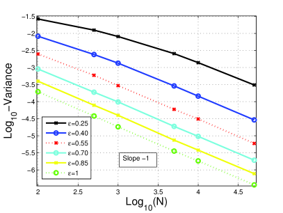
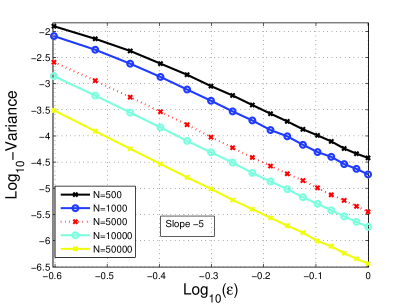
On Figure 1, we have reported the estimated variance error $V_{t}(\varepsilon,N)$ as a function of the particle number $N$, (on the left graph) and as a function of the regularization parameter $\varepsilon$, (on the right graph), for $t=T=1$ and $d=5$. We have used for this a similar Monte Carlo approximation as (5.33).
That figure shows that, when the number of particles is large enough, the variance error behaves precisely as in the classical case of density estimation encountered in [26], i.e., vanishing at a rate $\frac{1}{N\varepsilon^{d}}$, see relation (4.10), Chapter 4., Section 4.3.1. This is in particular illustrated by the log-log graphs, showing almost linear curve, when $N$ is sufficiently large. In particular we observe the following.

• On the left graph, $\log(V_{t}(\varepsilon,N))\approx a-\alpha\log N$ with slope $\alpha=1$;

• On the right graph, $\log V_{t}(\varepsilon,N)\approx b-\beta\log\varepsilon$ with slope $\beta=5=d$.

It seems that the threshold $N$ after which appears the linear behavior (compatible with the propagation of chaos situation corresponding to asymptotic-i.i.d. particles) decreases when $\varepsilon$ grows. In other words, when $\varepsilon$ is large, less particles $N$ are needed to give evidence to the chaotic behavior.

This phenomenon can be probably explained by analyzing the particle system dynamics. Indeed, at each time step, the interaction between the particles is due to the empirical estimation of $u^{\varepsilon}=K^{\varepsilon}\ast v^{\varepsilon}$ based on the particle system. Intuitively, the more accurate the approximation $u^{\varepsilon,N}$ of $u^{\varepsilon}$ is, the less strong the interaction between particles will be. In the limiting case when $u^{\varepsilon,N}=u^{\varepsilon}$, the interaction disappears.

Now observe that at time step $0$, the particle system $({\xi}^{i,N}_{0})$ is i.i.d. according to $v_{0}(\cdot)$, so that the estimation of $(K^{\varepsilon}\ast v^{\varepsilon})(0,\cdot)$ provided by (4.1) reduces to the classical density estimation approach, see [26] as mentioned above. In that classical framework, we emphasize that, for larger values of $\varepsilon$, the number of particles, needed to achieve a given density estimation accuracy, is smaller. Hence, one can imagine that for larger values of $\varepsilon$ less particles will be needed to obtain a quasi-i.i.d particle system at time step $1$, $({\xi}^{i,N}_{t_{1}})$. We can then reasonably presume that this initial error propagates along the time steps.

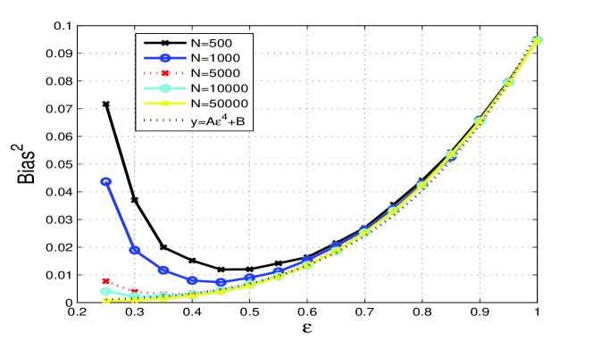
On Figure 2, we have reported the estimated squared bias error, $B^{2}_{t}(\varepsilon,N)$, as a function of the regularization parameter, $\varepsilon$, for different values of the particle number $N$, for $t=T=1$ and $d=5$.
One can observe that, similarly to the classical i.i.d. case, (see relation (4.9) in Chapter 4., Section 4.3.1 in [26]), for $N$ large enough, the bias error does not depend on $N$ and can be approximated by $a\varepsilon^{4}$, for some constant $a>0$. This is in fact coherent with the bias approximation (5.36), developed in the specific case where the weighting function $\Lambda$ does not depend on the density. Assuming the validity of approximation (5.36) and of the previous empirical observation implies that one can bound the error between the solution, $v^{\varepsilon}$, of the regularized PDE of the form (1.5) (with $K=K^{\varepsilon}$) associated to (5.27), and the solution, $v$, of the limit (non regularized) PDE (5.27) as follows

$$\|v_{t}^{\varepsilon}-v_{t}\|_{2}^{2} \leq 2\|v_{t}^{\varepsilon}-u_{t}^{\varepsilon}\|_{2}^{2}+2\|u_{t}^{\varepsilon}-v_{t}\|_{2}^{2}$$ (5.37)

$$\leq 2\|v_{t}^{\varepsilon}-K^{\varepsilon}\ast v_{t}^{\varepsilon}\|_{2}^{2}+2\|u_{t}^{\varepsilon}-v_{t}\|_{2}^{2}$$

$$\leq 2(a^{\prime}+a)\varepsilon^{4}.$$

Indeed, at least, the first term in the second line can be easily bounded, supposing that $v_{t}^{\varepsilon}$ has a bounded second derivative. This constitutes an empirical proof of the fact that $v^{\varepsilon}$ converges to $v$.
As observed in the variance error graphs, the threshold $N$, above which the propagation of chaos behavior is observed decreases with $\varepsilon$. Indeed, for $\varepsilon>0.6$ we observe a chaotic behavior of the bias error, starting from $N\geq 500$, whereas for $\varepsilon\in[0.4,0.6]$, this chaotic behavior appears only for $N\geq 5000$.
For small values of $\varepsilon\leq 0.6$, the bias highly depends on $N$ for any $N\leq 10^{4}$; moreover that dependence becomes less relevant when $N$ increases. This is probably due to the combination of two effects: the lack of chaos propagation phenomenon and the fact that the coefficient $\Lambda$ depends on $u$, so that (5.35) does not hold in that context.

Taking into account both the bias and the variance error in the MISE (5.34), the choice of $\varepsilon$ has to be carefully optimized w.r.t. the number of particles: $\varepsilon$ going to zero together with $N$ going to infinity at a judicious relative rate seem to ensure the convergence of the estimated MISE to zero. This kind of tradeoff is standard in density estimation theory and was already investigated theoretically in the context of forward interacting particle systems related to conservative regularized nonlinear PDE in [17]. Extending this type of theoretical analysis to our non conservative framework is beyond the scope of the present paper.

(a) Variance as a function of $N$

(b) Variance as a function of $\varepsilon$

Figure 1: Variance error as a function of the number of particles, $N$, and the mollifier window width, $\varepsilon$, for dimension $d=5$ at the final time step $T=1$.

Figure 2: Bias error as a function of the mollifier window width, $\varepsilon$, for dimension $d=5$ at the final time step $T=1$.

5.3.1 Time discretization error

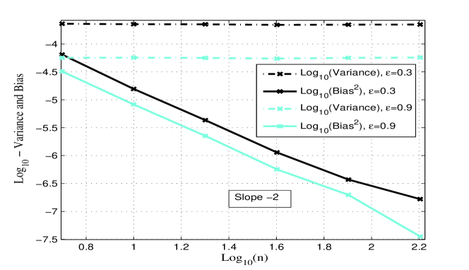
In this subsection, we are interested in analysing via numerical simulations the time discretization error w.r.t. to $\delta t={T}/{n}$. As announced in Remark 4.3, we suspect that the rate in (4.4) is not optimal and that the MISE error induced by the time discretization is of order $1/{n}^{2}$ instead of $1/{n}$.

Let $\tilde{u}^{\varepsilon,N,n}_{T}$ denote the particle approximation obtained by scheme (4.1) with a number of particles, $N$, a regularization parameter, $\varepsilon$, and a number of time steps, $n$. In order to focus on the time discretization error apart from the particle approximation and the regularization error (related to $N$ and $\varepsilon$), we have considered errors of the type $\mathbb{E}[\|\tilde{u}^{\varepsilon,N,n}_{T}-\tilde{u}_{T}^{\varepsilon,N,n_{0}}\|^{2}_{2}]$ for different numbers of time steps $n<n_{0}$ where $n_{0}$ is supposed to be a large number of time steps. More precisely, we have decomposed this error into a variance and a squared bias term as

$$\mathbb{E}[\|\tilde{u}^{\varepsilon,N,n}_{T}-\tilde{u}_{T}^{\varepsilon,N,n_{0}}\|^{2}_{2}] = \underbrace{\mathbb{E}\big{[}\|\tilde{u}^{\varepsilon,N,n}_{T}-\mathbb{E}[\tilde{u}_{T}^{\varepsilon,N,n}]\|^{2}_{2}\big{]}+\mathbb{E}\big{[}\|\tilde{u}^{\varepsilon,N,n_{0}}_{T}-\mathbb{E}[\tilde{u}_{T}^{\varepsilon,N,n_{0}}]\|^{2}_{2}\big{]}}_{\textrm{Variance}}$$

$$+ \underbrace{\|\mathbb{E}[\tilde{u}^{\varepsilon,N,n}_{T}]-\mathbb{E}[\tilde{u}_{T}^{\varepsilon,N,n_{0}}]\|^{2}_{2}}_{\textrm{Bias}^{2}},$$

if $u^{\varepsilon,N,n}_{T}$ and $u^{\varepsilon,N,n_{0}}_{T}$ are independent.

On Figure 3, we have reported the Monte Carlo estimation (according to (5.33), with $Q=1000$ runs) of the above variance and squared bias terms in a log-log scale in order to diagnose the expected rate of convergence $1/{n}^{2}$ via a straight line with slope $-2$. All the parameters are similar to the simulations performed in previous subsection excepted for the dimension $d=1,N=5000$ and $n_{0}$ is set to $1000$ time steps. One can observe that the variance term (in dashed lines) seems not to depend on the number of time steps $n$ whereas the squared bias term decreases as expected at a rate close to $1/n^{2}$.

Figure 3: Variance and squared bias error (5.3.1) as a function of the number of time steps, $n=5,10,20,40,80,160,320$, at the final time step $T=1$ (with dimension $d=1$, $N=5000$ particles and $\varepsilon=0.3$ or $0.9$).

6 Appendix

In this appendix, we present the proof of Lemma 4.4. We first proceed with the proof of some intermediary inequalities.

Lemma 6.1.

We suppose Assumption 1. Let $N\in\mathbb{N}^{\star}$. Let $(\xi^{i,N})_{i=1,\cdots,N}$ be (a solution of) the interacting particle system (3.3); let $(\tilde{\xi}^{i,N})_{i=1,\cdots,N}$ and $\tilde{u}$ as defined as in the discretized interacting particle system (4.1).
The random variables $V_{t}^{i}:=e^{\int_{0}^{t}\Lambda\big{(}s,\tilde{\xi}^{i,N}_{s},u^{S^{N}(\tilde{\xi})}_{s}(\tilde{\xi}^{i,N}_{s})\big{)}ds}$ and $\tilde{V}_{t}^{i}:=e^{\int_{0}^{t}\Lambda\big{(}r(s),\tilde{\xi}^{i,N}_{r(s)},\tilde{u}_{r(s)}(\tilde{\xi}^{i,N}_{r(s)})\big{)}ds}$, for all $t\in[0,T]$, $i\in\{1,\cdots,N\}$ fulfill the following.

1. For all $t\in[0,T]$, $i\in\{1,\cdots,N\}$

   $$\mathbb{E}[|\tilde{V}_{t}^{i}-V_{t}^{i}|^{2}]\leq C\delta t+C\mathbb{E}\left[\int_{0}^{t}|\tilde{\xi}^{i,N}_{r(s)}-\tilde{\xi}^{i,N}_{s}|^{2}\ ds\right]+C\mathbb{E}\left[\int_{0}^{t}|\tilde{u}_{r(s)}(\tilde{\xi}^{i,N}_{r(s)})-u^{S^{N}(\tilde{\xi})}_{s}(\tilde{\xi}^{i,N}_{s})|^{2}ds\right],$$ (6.1)

   where $C$ is a real positive constant depending only on $M_{\Lambda}$, $L_{\Lambda}$ and $T$.

2. For all $(t,y)\in[0,T]\times\mathbb{R}^{d}$, $i\in\{1,\cdots,N\}$

   $$|\tilde{u}_{t}(y)-u_{t}^{S^{N}(\tilde{\xi})}(y)|^{2}\leq\frac{M_{K}}{N}\sum_{i=1}^{N}K(y-\tilde{\xi}^{i,N}_{t})\;|\tilde{V}_{t}^{i}-V_{t}^{i}|^{2}\ .$$ (6.2)

Proof of Lemma 6.1.

Let us fix $t\in[0,T]$, $i\in\{1,\cdots,N\}$. To prove (6.1), it is enough to recall that $\Lambda$ being Lipschitz w.r.t. the space variables and $\frac{1}{2}$-Holder continuous w.r.t. the time variable, the inequality (2.6) yields

$$|\tilde{V}_{t}^{i}-V_{t}^{i}|^{2}\leq 3e^{2tM_{\Lambda}}L^{2}_{\Lambda}\int_{0}^{t}\left[|r(s)-s|+|\tilde{\xi}^{i,N}_{r(s)}-\tilde{\xi}^{i,N}_{s}|^{2}+|\tilde{u}_{r(s)}(\tilde{\xi}^{i,N}_{r(s)})-u_{s}^{S^{N}(\tilde{\xi})}(\tilde{\xi}^{i,N}_{s})|^{2}\right]\,ds\ ,$$ (6.3)

and taking the expectation in both sides of (6.3) implies (6.1) with $C:=3e^{2TM_{\Lambda}}L^{2}_{\Lambda}$.
Let us fix $y\in\mathbb{R}^{d}$. Concerning (6.2), by recalling the third line equation of (4.1) and the linking equation (1.6) (with $m=S^{N}(\tilde{\xi})$), we have

$$|\tilde{u}_{t}(y)-u_{t}^{S^{N}(\tilde{\xi})}(y)|^{2} = \left|\frac{1}{N}\sum_{i=1}^{N}K(y-\tilde{\xi}_{t}^{i,N})\tilde{V}^{i}_{t}-\frac{1}{N}\sum_{i=1}^{N}K(y-\tilde{\xi}_{t}^{i,N})V^{i}_{t}\right|^{2}$$ (6.4)

$$= \left|\frac{1}{N}\sum_{i=1}^{N}K(y-\tilde{\xi}_{t}^{i,N})\left(\tilde{V}^{i}_{t}-V^{i}_{t}\right)\right|^{2}$$

$$\leq \frac{1}{N}\sum_{i=1}^{N}K^{2}(y-\tilde{\xi}^{i,N}_{t})|\tilde{V}_{t}^{i}-V_{t}^{i}|^{2}$$

$$\leq \frac{M_{K}}{N}\sum_{i=1}^{N}K(y-\tilde{\xi}^{i,N}_{t})\;|\tilde{V}_{t}^{i}-V_{t}^{i}|^{2}\ ,$$

which concludes the proof of (6.2) and therefore of Lemma 6.1. ∎

Proof of Lemma 4.4..

All along this proof, $C$ will denote a positive constant that only depends
$T,M_{K},m_{\Phi},m_{g},L_{K},L_{\Phi},L_{g}$ and $M_{\Lambda},L_{\Lambda}$ and that can change from line to line.
Let us fix $t\in[0,T]$.

• Inequality (4.8) of Lemma 4.4 is simply a consequence of the following computation:

  $$\mathbb{E}[|\tilde{\xi}^{i,N}_{r(t)}-\tilde{\xi}^{i,N}_{t}|^{2}] = \mathbb{E}\left[\Big{|}\int_{r(t)}^{t}\Phi(r(s),\tilde{\xi}^{i,N}_{r(s)},\tilde{u}_{r(s)}(\tilde{\xi}^{i,N}_{r(s)}))\,dW_{s}+\int_{r(t)}^{t}g(r(s),\tilde{\xi}^{i,N}_{r(s)},\tilde{u}_{r(s)}(\tilde{\xi}^{i,N}_{r(s)}))\,ds\Big{|}^{2}\right]$$

  $$\leq 4\mathbb{E}\left[\int_{r(t)}^{t}|\Phi(r(s),\tilde{\xi}^{i,N}_{r(s)},\tilde{u}_{r(s)}(\tilde{\xi}^{i,N}_{r(s)}))-\Phi(r(s),0,0)|^{2}\,ds\right]+4\mathbb{E}\left[\int_{r(t)}^{t}|\Phi(r(s),0,0)|^{2}\,ds\right]$$

  $$\;+4(t-r(t))\mathbb{E}\left[\int_{r(t)}^{t}|g(r(s),\tilde{\xi}^{i,N}_{r(s)},\tilde{u}_{r(s)}(\tilde{\xi}^{i,N}_{r(s)}))-g(r(s),0,0)|^{2}\,ds\right]$$

  $$\;+4(t-r(t))\mathbb{E}\left[\int_{r(t)}^{t}|g(r(s),0,0)|^{2}\,ds\right]$$

  $$\leq 8(L_{\Phi}^{2}+(t-r(t))L_{g}^{2})\int_{r(t)}^{t}\mathbb{E}\Big{[}|\tilde{\xi}^{i,N}_{r(s)}|^{2}\Big{]}+\mathbb{E}\Big{[}|\tilde{u}_{r(s)}(\tilde{\xi}^{i,N}_{r(s)})|^{2}\Big{]}ds$$

  $$+\;4(t-r(t))\Big{(}\sup_{s\in[0,T]}|\Phi(s,0,0)|^{2}+(t-r(t))\sup_{s\in[0,T]}|g(s,0,0)|^{2}\Big{)}$$

  $$\leq C\delta t\ ,\quad\textrm{as soon as }\quad\delta t\in\,]0,1[\ ,$$

  where we have used the fact, under items 1. and 6. of Assumption 2, that the second order moment of $\tilde{\xi}^{i,N}_{s}$ is uniformly bounded. $\Lambda$ being uniformly bounded (item 3. of Assumption 2), the function $\tilde{u}$ as well. We have finally invoked item 6. of Assumption 2.

• Now, let us focus on the second inequality (4.9) of Lemma 4.4. Note that for any $y\in\mathbb{R}^{d}$, the following inequality holds:

  $$|\tilde{u}_{r(t)}(y)-\tilde{u}_{t}(y)| \leq \frac{1}{N}\sum_{i=1}^{N}\left[\left|K(y-\tilde{\xi}^{i,N}_{r(t)})-K(y-\tilde{\xi}^{i,N}_{t})\right|\,e^{\int_{0}^{r(t)}\Lambda\big{(}r(s),\tilde{\xi}^{i,N}_{r(s)},\tilde{u}_{r(s)}(\tilde{\xi}^{i,N}_{r(s)})\big{)}ds}\right.$$

  $$+\left.K(y-\tilde{\xi}^{i,N}_{t})\,\left|e^{\int_{0}^{r(t)}\Lambda\big{(}r(s),\tilde{\xi}^{i,N}_{r(s)},\tilde{u}_{r(s)}(\tilde{\xi}^{i,N}_{r(s)})\big{)}ds}-e^{\int_{0}^{t}\Lambda\big{(}r(s),\tilde{\xi}^{i,N}_{r(s)},\tilde{u}_{r(s)}(\tilde{\xi}^{i,N}_{r(s)})\big{)}ds}\right|\right]\ .$$

  Using the fact that $K$ and $\Lambda$ are bounded, one can apply (2.6) to bound the second term of the sum on the r.h.s. of the above inequality as follows:

  $$K(y-\tilde{\xi}^{i,N}_{t})\,\left|e^{\int_{0}^{r(t)}\Lambda\big{(}r(s),\tilde{\xi}^{i,N}_{r(s)},\tilde{u}_{r(s)}(\tilde{\xi}^{i,N}_{r(s)})\big{)}ds}-e^{\int_{0}^{t}\Lambda\big{(}r(s),\tilde{\xi}^{i,N}_{r(s)},\tilde{u}_{r(s)}(\tilde{\xi}^{i,N}_{r(s)})\big{)}ds}\right| \leq M_{K}e^{tM_{\Lambda}}(t-r(t))M_{\Lambda}$$ (6.6)

  $$\leq C\delta t\ .$$

  The first term of the sum on the r.h.s. of (• ‣ 6) is bounded using the Lipschitz property of $K$ and the fact that $\Lambda$ is bounded.

  $$\left|K(y-\tilde{\xi}^{i,N}_{r(t)})-K(y-\tilde{\xi}^{i,N}_{t})\right|\,e^{\int_{0}^{r(t)}\Lambda\big{(}r(s),\tilde{\xi}^{i,N}_{r(s)},\tilde{u}_{r(s)}(\tilde{\xi}^{i,N}_{r(s)})\big{)}ds}\leq L_{K}e^{tM_{\Lambda}}|\tilde{\xi}^{i,N}_{r(t)}-\tilde{\xi}^{i,N}_{t}|\ .$$ (6.7)

  Injecting (6.6) and (6.7) in (• ‣ 6), for all $y\in\mathbb{R}^{d}$, we obtain

  $$|\tilde{u}_{r(t)}(y)-\tilde{u}_{t}(y)|\leq C\delta t+\frac{L_{K}e^{tM_{\Lambda}}}{N}\sum_{i=1}^{N}|\tilde{\xi}^{i,N}_{r(t)}-\tilde{\xi}^{i,N}_{t}|,$$

  which finally implies that

  $$\|\tilde{u}_{r(t)}-\tilde{u}_{t}\|_{\infty}^{2}\leq C\delta t^{2}+\frac{C}{N}\sum_{i=1}^{N}|\tilde{\xi}^{i,N}_{r(t)}-\tilde{\xi}^{i,N}_{t}|^{2}\ .$$

  We conclude by using inequality (4.8) of Lemma 4.4 after taking the expectation of the r.h.s. of the above inequality.

• Finally, we deal with inequality (4.10) of Lemma 4.4. Observe that the error on the left-hand side can be decomposed as

  $$\mathbb{E}[\|\tilde{u}_{r(t)}-u_{t}^{S^{N}(\tilde{\xi})}\|^{2}_{\infty}] \leq 2\mathbb{E}[\|\tilde{u}_{r(t)}-\tilde{u}_{t}\|^{2}_{\infty}]+2\mathbb{E}[\|\tilde{u}_{t}-u_{t}^{S^{N}(\tilde{\xi})}\|^{2}_{\infty}]$$ (6.8)

  $$\leq C\delta t+2\mathbb{E}[\|\tilde{u}_{t}-u_{t}^{S^{N}(\tilde{\xi})}\|^{2}_{\infty}]\ ,$$

  where we have used inequality (4.9) of Lemma 4.4.
  Let us consider the second term on the r.h.s. of the above inequality. To simplify the notations, we introduce the real valued random variables

  $$V_{t}^{i}:=e^{\int_{0}^{t}\Lambda\big{(}s,\tilde{\xi}^{i,N}_{s},u^{S^{N}(\tilde{\xi})}_{s}(\tilde{\xi}^{i,N}_{s})\big{)}ds}\quad\textrm{and}\quad\tilde{V}_{t}^{i}:=e^{\int_{0}^{t}\Lambda\big{(}r(s),\tilde{\xi}^{i,N}_{r(s)},\tilde{u}_{r(s)}(\tilde{\xi}^{i,N}_{r(s)})\big{)}ds}\ ,$$ (6.9)

  defined for any $i=1,\cdots N$ and $t\in[0,T]$.
  Using successively inequalities (6.1) of Lemma 6.1, (4.8) of Lemma 4.4 and (2.9) of Proposition 2.5, we have for all $i\in\{1,\cdots,N\}$,

  $$\mathbb{E}[|\tilde{V}_{t}^{i}-V_{t}^{i}|^{2}] \leq C\delta t+C\mathbb{E}\left[\int_{0}^{t}|\tilde{u}_{r(s)}(\tilde{\xi}^{i,N}_{r(s)})-u^{S^{N}(\tilde{\xi})}_{s}(\tilde{\xi}^{i,N}_{s})|^{2}ds\right]$$ (6.10)

  $$\leq C\delta t+C\mathbb{E}\left[\int_{0}^{t}|\tilde{u}_{r(s)}(\tilde{\xi}^{i,N}_{r(s)})-u^{S^{N}(\tilde{\xi})}_{s}(\tilde{\xi}^{i,N}_{r(s)})|^{2}ds\right]$$

  $$+\;C\mathbb{E}\left[\int_{0}^{t}|u_{s}^{S^{N}(\tilde{\xi})}(\tilde{\xi}^{i,N}_{r(s)})-u^{S^{N}(\tilde{\xi})}_{s}(\tilde{\xi}^{i,N}_{s})|^{2}ds\right]$$

  $$\leq C\delta t+C\int_{0}^{t}\left[\mathbb{E}[\|\tilde{u}_{r(s)}-u^{S^{N}(\tilde{\xi})}_{s}\|_{\infty}^{2}]+\mathbb{E}[|\tilde{\xi}^{i,N}_{r(s)}-\tilde{\xi}^{i,N}_{s}|^{2}]\right]\,ds$$

  $$\leq C\delta t+C\int_{0}^{t}\mathbb{E}[\|\tilde{u}_{r(s)}-u^{S^{N}(\tilde{\xi})}_{s}\|_{\infty}^{2}]\,ds\ .$$

  On the other hand, inequality (6.2) of Lemma 6.1 implies

  $$\|\tilde{u}_{t}-u_{t}^{S^{N}(\tilde{\xi})}\|_{\infty}^{2}\leq\frac{M_{K}^{2}}{N}\sum_{i=1}^{N}|\tilde{V}_{t}^{i}-V_{t}^{i}|^{2}\ .$$ (6.11)

  Taking the expectation in both sides of (6.11) and using (6.10) give

  $$\mathbb{E}[\|\tilde{u}_{t}-u_{t}^{S^{N}(\tilde{\xi})}\|^{2}_{\infty}]\leq\frac{M_{K}^{2}}{N}\sum_{i=1}^{N}\mathbb{E}\left[|\tilde{V}_{t}^{i}-V_{t}^{i}|^{2}\right]\leq C\delta t+C\int_{0}^{t}\mathbb{E}[\|\tilde{u}_{r(s)}-u^{S^{N}(\tilde{\xi})}_{s}\|_{\infty}^{2}]\,ds\ .$$ (6.12)

  We end the proof by injecting this last inequality in (6.8) and by applying Gronwall’s lemma.

∎

ACKNOWLEDGEMENTS. The authors are very grateful to the anonymous Referee for her / his careful reading of the paper and the suggestions which have largely contributed to improve the first submitted version. The third named author has benefited partially from the support of the “FMJH Program Gaspard Monge in optimization and operation research” (Project 2014-1607H).

References

- [1] G. I. Barenblatt. On some unsteady motions of a liquid and gas in a porous medium. Akad. Nauk SSSR. Prikl. Mat. Meh., 16:67–78, 1952.
- [2] N. Belaribi, F. Cuvelier, and F. Russo. A probabilistic algorithm approximating solutions of a singular PDE of porous media type. Monte Carlo Methods and Applications, 17(4):317–369, 2011.
- [3] N. Belaribi, F. Cuvelier, and F. Russo. Probabilistic and deterministic algorithms for space multidimensional irregular porous media equation. SPDEs: Analysis and Computations, 1(1):3–62, 2013.
- [4] M. Ben Alaya and B. Jourdain. Probabilistic approximation of a nonlinear parabolic equation occurring in rheology. J. Appl. Probab., 44(2):528–546, 2007.
- [5] D. P. Bertsekas and S. E. Shreve. Stochastic optimal control, volume 139 of Mathematics in Science and Engineering. Academic Press, Inc. [Harcourt Brace Jovanovich, Publishers], New York-London, 1978. The discrete time case.
- [6] M. Bossy and B. Jourdain. Rate of convergence of a particle method for the solution of a 1D viscous scalar conservation law in a bounded interval. Ann. Probab., 30(4):1797–1832, 2002.
- [7] M. Bossy and D. Talay. A stochastic particle method for some one-dimensional nonlinear p.d.e. Math. Comput. Simulation, 38(1-3):43–50, 1995. Probabilités numériques (Paris, 1992).
- [8] M. Bossy and D. Talay. A stochastic particle method for the McKean-Vlasov and the Burgers equation. Math. Comp., 66(217):157–192, 1997.
- [9] B. Bouchard and N. Touzi. Discrete-time approximation and Monte Carlo simulation of backward stochastic differential equations. Stochastic Process. Appl., 111:175–206, 2004.
- [10] P. Cheridito, H. M. Soner, N. Touzi, and N. Victoir. Second-order backward stochastic differential equations and fully nonlinear parabolic PDEs. Comm. Pure Appl. Math., 60(7):1081–1110, 2007.
- [11] H. Crauel. Random probability measures on Polish spaces, volume 11 of Stochastics Monographs. Taylor & Francis, London, 2002.
- [12] P. Del Moral. Feynman-Kac formulae. Probability and its Applications (New York). Springer-Verlag, New York, 2004. Genealogical and interacting particle systems with applications.
- [13] P. Del Moral. Mean field simulation for Monte Carlo integration, volume 126 of Monographs on Statistics and Applied Probability. CRC Press, Boca Raton, FL, 2013.
- [14] E. Gobet, J-P. Lemor, and X. Warin. A regression-based Monte Carlo method to solve backward stochastic differential equations. Ann. Appl. Probab., 15(3):2172–2202, 2005.
- [15] P. Henry-Labordère. Counterparty risk valuation: A marked branching diffusion approach. Available at SSRN: http://ssrn.com/abstract=1995503 or http://dx.doi.org/10.2139/ssrn.1995503, 2012.
- [16] P. Henry-Labordère, X. Tan, and N. Touzi. A numerical algorithm for a class of BSDEs via the branching process. Stochastic Process. Appl., 124(2):1112–1140, 2014.
- [17] B. Jourdain and S. Méléard. Propagation of chaos and fluctuations for a moderate model with smooth initial data. Ann. Inst. H. Poincaré Probab. Statist., 34(6):727–766, 1998.
- [18] I. Karatzas and S. E. Shreve. Brownian motion and stochastic calculus, volume 113 of Graduate Texts in Mathematics. Springer-Verlag, New York, second edition, 1991.
- [19] A. Kohatsu-Higa and S. Ogawa. Weak rate of convergence for an Euler scheme of nonlinear SDE’s. Monte Carlo Methods Appl., 3(4):327–345, 1997.
- [20] A. Le Cavil, N. Oudjane, and F. Russo. Probabilistic representation of a class of non conservative nonlinear partial differential equations. Preprint HAL. https://hal.archives-ouvertes.fr/hal-01241701, 2015.
- [21] H. P. Jr. McKean. Propagation of chaos for a class of non-linear parabolic equations. In Stochastic Differential Equations (Lecture Series in Differential Equations, Session 7, Catholic Univ., 1967), pages 41–57. Air Force Office Sci. Res., Arlington, Va., 1967.
- [22] E. Pardoux. Backward stochastic differential equations and viscosity solutions of systems of semilinear parabolic and elliptic PDEs of second order. In Stochastic analysis and related topics, VI (Geilo, 1996), volume 42 of Progr. Probab., pages 79–127. Birkhäuser Boston, Boston, MA, 1998.
- [23] É. Pardoux and S. G. Peng. Adapted solution of a backward stochastic differential equation. Systems Control Lett., 14(1):55–61, 1990.
- [24] E. Pardoux and A. Raşcanu. Stochastic differential equations, Backward SDEs, Partial differential equations, volume 69. Springer, 2014.
- [25] L. C. G. Rogers and D. Williams. Diffusions, Markov processes, and martingales. Vol. 2. Cambridge Mathematical Library. Cambridge University Press, Cambridge, 2000. Itô calculus, Reprint of the second (1994) edition.
- [26] B. W. Silverman. Density estimation for statistics and data analysis. Monographs on Statistics and Applied Probability. Chapman & Hall, London, 1986.
- [27] A-S. Sznitman. Topics in propagation of chaos. In École d’Été de Probabilités de Saint-Flour XIX—1989, volume 1464 of Lecture Notes in Math., pages 165–251. Springer, Berlin, 1991.
- [28] D. Talay. Probabilistic numerical methods for partial differential equations: elements of analysis. In Probabilistic models for nonlinear partial differential equations (Montecatini Terme, 1995), volume 1627 of Lecture Notes in Math., pages 148–196. Springer, Berlin, 1996.