Multi-task Prediction of Disease Onsets from Longitudinal Lab Tests

Abstract

Disparate areas of machine learning have benefited from models that can take raw data with little preprocessing as input and learn rich representations of that raw data in order to perform well on a given prediction task. We evaluate this approach in healthcare by using longitudinal measurements of lab tests, one of the more raw signals of a patient’s health state widely available in clinical data, to predict disease onsets. In particular, we train a Long Short-Term Memory (LSTM) recurrent neural network and two novel convolutional neural networks for multi-task prediction of disease onset for 133 conditions based on 18 common lab tests measured over time in a cohort of 298K patients derived from 8 years of administrative claims data. We compare the neural networks to a logistic regression with several hand-engineered, clinically relevant features. We find that the representation-based learning approaches significantly outperform this baseline. We believe that our work suggests a new avenue for patient risk stratification based solely on lab results.

1 Introduction

The recent success of deep learning in disparate areas of machine learning has driven a shift towards machine learning models that can learn rich, hierarchical representations of raw data with little preprocessing and away from models that require manual construction of features by experts (Graves and Schmidhuber, 2005; Krizhevsky et al., 2012; Mikolov et al., 2013). In natural language processing, for example, neural networks taking only character-level input achieve high performance on many tasks including text classification tasks (Zhang et al., 2015; Kim, 2014), machine translation (Ling et al., 2015) and language modeling (Kim et al., 2016).

Following these advances, attempts to learn features from raw medical signals have started to gain attention too. Lasko et al. (2013) studied a method based on sparse auto-encoders to learn temporal variation features from 30-day uric acid observations to distinguish between gout and leukemia. Che et al. (2015) developed a training method which, when datasets are small, allows prior domain knowledge to regularize the deeper layers of a feed-forward network for the task of multiple disease classification. Recent studies (Lipton et al., 2015; Choi et al., 2015) used Long Short-Term Memory (LSTM) recurrent neural networks (RNNs) for disease phenotyping.

In this paper, we evaluate the representation-based learning approach in healthcare by using longitudinal measurements of laboratory tests, one of the more raw signals of a patient’s health state widely available in clinical data, to predict disease onsets. We show that several multi-task neural networks, including a LSTM RNN and two novel convolutional neural networks, can aid in early diagnosis of a wide range of conditions (including conditions that the patient was not specifically tested for) without having to hand-engineer features for each condition. The source code of our implementation is available at https://github.com/clinicalml/deepDiagnosis.

2 Prediction Task

Figure 1 outlines the study’s prediction framework. Our goal is early diagnosis of diseases for people who do not already have the disease. We required a 3-month gap between the end of the backward window, denoted $t$, and the start of the diagnosis window. The purpose of the 3 month gap was to ensure that the clinical tests taken right before the diagnosis of a disease would not allow our system to cheat in the prediction of that disease. Each output label was defined as positive if the diagnosis code for the disease was observed in at least $2$ distinct months between $3$ to $3+12$ months after $t$. Using $12$ months helps alleviate the noisy label problem. Requiring at least $2$ observations of the code also reduced the noise coming from physicians who report their wrong suspected diagnosis as a diagnosis. For each disease, we excluded individuals who already have the disease by time $t+3$. For exclusion, we required only $1$ diagnosis record instead of $2$ in order to remove patients who are even suspected of having the disease previously. This results in a more difficult, but more clinically meaningful prediction task.

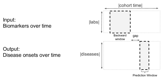
Figure 1: Overview of our prediction framework.

Formally, we define the task of diagnosis as a supervised multi-task sequence classification problem. Each individual has a variable-length history of lab observations ($X$) and diagnosis records ($Y$). $X$ is continuous valued and $Y$ is binary. We use a sliding window framework to deal with variable length input. At each time point $t$ for each person, the model looks at a backward window of $B$ months of all $D$ biomarkers of the input, $X_{t-B:t}^{1:D}$, to predict the output. The output is a binary vector $Y$ of length $M$ indicating for each of the $M$ diseases whether they are newly diagnosed in the following months $t+3$ to $t+3+12$, where $3$ is the gap and $12$ is the prediction window.

3 Cohort

Our dataset consisted of lab measurement and diagnosis information for 298,000 individuals. The lab measurements had the resolution of 1 month and we used a backward window of 36 months for each prediction. These individuals were selected from a larger cohort of 4.1 million insurance subscribers between 2005 and 2013. We only included members who had at least one lab measurement per year for at least 3 consecutive years.

We used lab tests that comprise a comprehensive metabolic panel plus cholesterol and bilirubin (18 lab tests in total), which are currently recommended annually and covered by most insurance companies in the United States. The names and codes of the labs used in our analysis are included in the Supplementary Materials. Each lab value was normalized by subtracting its mean and dividing by the standard deviation computed across the entire dataset. We randomly divided individuals into a 100K training set, a 100K validation set, and a 98K test set. The validation set was used to select the best epoch/parameters for models and prediction results are presented on the test set unseen during training and validation.

The predicted labels corresponded to diagnosis information for these individuals. In our dataset, each disease diagnosis is recorded as an ICD9-CM (International Classification of Diseases, Ninth Revision, Clinical Modification) code.

4 Methods

We now describe the baseline model, the two novel convolutional (Le Cun et al., 1990; LeCun et al., 1998) architectures and the recurrent neural network with long short-term memory units (Hochreiter and Schmidhuber, 1997) that we evaluate on this prediction task. The input to the baseline model are hand-engineered features derived from the patient’s lab measurements, whereas the input to the representation-based models are the raw, sparse and asynchronously measured lab measurements. We also report the results of an ensemble of the representation-based models.

4.1 Baseline

We trained a Logistic Regression model on a large set of features derived from the patient’s lab measurements. These features included the minimum, maximum and latest observation value for each of the labs as well as binary indicators for increasing and decreasing trends in the lab values within the backward window. The continuous features were computed on lab values that were normalized across the cohort (to have zero mean and unit variance). We used the validate data to choose the type and amount of L1, L2, and Dropout (Srivastava et al., 2014) regularization, separately for each disease.

4.2 Multi-resolution Convolutional Neural Network (CNN1)

The architecture for our first convolutional neural network is shown in Figure 2. We define $X_{t-B:t}^{1:D}$ to be the input to the network at time $t$ for $D$ lab measurements over the past $B$ months. Let $J$ be the number of filters in each convolution operator. Each filter $K_{i}^{j}$ ($j=1:J$) is of size $1\times L$. The output of the convolution part of the network is a vector $C=[C_{1},C_{2},C_{5}]$ which is defined as follows:

$$C_{1}^{d,j}= f(b_{1}^{j}+K_{1}^{j}*\textrm{MaxPool}(X_{t-B:t}^{d},p^{2}))$$ (1)

$$C_{2}^{d,j}= f(b_{2}^{j}+K_{2}^{j}*\textrm{MaxPool}(X_{t-B:t}^{d},p))$$ (2)

$$C_{3}^{d,j}= f(b_{3}^{j}+K_{3}^{j}*X_{t-B:t}^{1:D})$$ (3)

$$C_{4}^{d,j}= \textrm{MaxPool}(C_{3}^{d,j},p)$$ (4)

$$C_{5}^{d,j}= f(b_{5}^{j}+\sum_{k=1}^{J}K^{j}_{5}*C_{4}^{d,k})$$ (5)

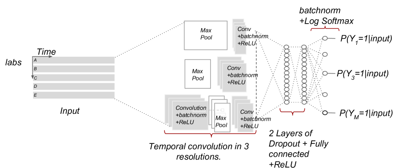
Figure 2: Architecture for Multi-resolution Convolutional Neural Network (CNN1)

In the equations above, the nonlinearity $f$ is a rectified linear unit (ReLU) (Nair and Hinton, 2010) applied element-wise to a vector, and $*$ is the standard convolution operation. $\textrm{MaxPool}(Z,s)$ corresponds to a non-overlapping max pooling operation with step size $k$, defined as $\textrm{MaxPool}(Z,s)[i]=\max(Z_{i\cdot s},\ldots,Z_{(i+1)\cdot s-1})$ for $i=1:\lfloor\textrm{length}(Z)/s\rfloor$. We set $p=3$ for this paper. The vector $C_{i}$ is the concatenation of $C_{i}^{d,j}$ for all labs $d=1:D$ and filters $j=1:J$. The outputs of the first and second level in the multi-resolution network, ($C_{1},C_{2}$), are results of the convolution operator applied to kernels $K_{1}^{j}$ and $K_{2}^{j}$ at different resolutions of the input. The third level of resolution includes two layers of convolution using filters $K_{3}^{j}$ and $K_{5}^{j}$. After every convolution operation, we use batch normalization (Ioffe and Szegedy, 2015).

After the multi-resolution convolution is applied, the vector $C=[C_{1},C_{2},C_{5}]$ represents the application of filters to all labs (note that the filters are shared across all the labs). We then use $2$ layers of hidden nodes to allow non-linear combination of filter activations on different labs:

$$h_{1}= f(W_{1}^{T}C+b_{h_{1}})$$ (6)

$$h_{2}= f(W_{2}^{T}h_{1}+b_{h_{2}})$$ (7)

$W_{i}$ are the weights for the hidden nodes and $b_{h_{i}}$ is the bias associated with each layer. Each of the hidden layers are subject to Dropout regularization (with probability 0.5) during training, and are followed by batch normalization.

Finally, for each disease $m=1:M$, the model predicts the likelihood of the disease via logistic regression over $h_{2}$:

$$P(Y_{m}=1|X_{t-B:t}^{1:D})=\sigma(W_{m}^{T}h_{2}+b_{m}),$$ (8)

where $\sigma(x)=1/(1+e^{-x})$ is the sigmoid function. The loss function for each disease is the negative log likelihood of the true label, weighted by the inverse-label frequency to handle class imbalance during multi-task batch training. Diseases are trained independently, but the gradient is backpropagated through the shared part of the network for all diseases.

4.3 Convolutional Neural Network over Time and Input dimensions (CNN2)

The architecture for our second convolutional neural network is shown in Figure 3. In this model, we first combine the labs via a vertical convolution with kernels that span across all labs. Having a few such combination layers enables us to project from the lab space into a new latent space which might better encode information about the labs. We then focus on temporal encoding of the result in the new space.

Given the input $X_{t-B:t}^{1:D}$, the output of the first vertical convolution with $L$ filters $K^{1:L}$, each of size ($D\times 1$), and nonlinearity $f$ is $V_{1:L}^{t-B:t}$ of size ($L\times 1\times B$), where

$$V_{l}^{t-B:t}=f(b_{l}+K^{l}*X_{t-B:t}^{1:D})$$ (9)

Figure 3: Architecture for Convolutional Neural Network over Time and Input dimensions (CNN2)

for $l=1:L$. We then repeat, applying new convolution filters of size $L\times 1$ to $V_{1:L}^{t-B:t}$, followed again by a nonlinearity $f$ (ReLU in our experiments), giving us two hidden layers in the vertical direction. Finally, temporal max pooling and convolution is applied to the last convolution output followed by two fully connected layers, similar to equations (2) and (6) through (8). Similar to the previous architecture, we optimize the weighted negative log-likelihood of the disease labels on the training data.

4.4 Long Short-Term Memory Network (LSTM)

The architecture for the Recurrent Neural Network with Long Short-Term Memory units (Hochreiter and Schmidhuber, 1997) is shown in Figure 4. These models encode a memory state $c_{\hat{t}}$ at each time step $\hat{t}$, which is only accessible through a particular gating mechanism. Given input $X_{\hat{t}}$ and the output and memory state of the recurrent network at time $\hat{t}-1$ ($h_{\hat{t}-1}$), the memory state and output for time steps $\hat{t}:t-B:t$ are computed as follows:

$$i_{\hat{t}}= \sigma(W_{x\rightarrow i}X_{\hat{t}}+W_{h\rightarrow i}h_{\hat{t}-1}+W_{c\rightarrow i}c_{\hat{t}-1}+b_{1\rightarrow i})$$ (10)

$$f_{\hat{t}}= \sigma(W_{x\rightarrow f}X_{\hat{t}}+W_{h\rightarrow f}h_{\hat{t}-1}+W_{c\rightarrow f}c_{\hat{t}-1}+b_{1\rightarrow f})$$ (11)

$$z_{\hat{t}}= \tanh(W_{x\rightarrow c}X_{\hat{t}}+W_{h\rightarrow c}h_{\hat{t}-1}+b_{1\rightarrow c})$$ (12)

$$c_{\hat{t}}= f_{\hat{t}}c_{\hat{t}−1}+i_{\hat{t}}z_{\hat{t}}$$ (13)

$$o_{\hat{t}}= \sigma(W_{x\rightarrow o}X_{\hat{t}}+W_{h\rightarrow o}h_{\hat{t}-1}+W_{c\rightarrow o}c_{\hat{t}}+b_{1\rightarrow o})$$ (14)

$$h_{\hat{t}}= o_{\hat{t}}\tanh(c_{\hat{t}})$$ (15)

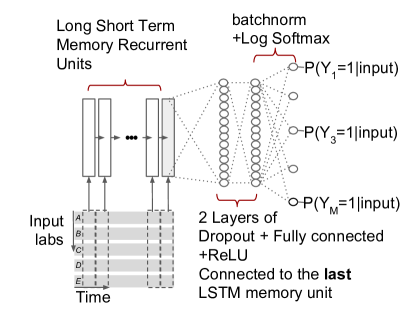
Figure 4: Architecture for the Long Short-Term Memory Network (LSTM)

where $W_{*}$ and $b_{*}$ are the network’s parameters, shared across all time steps. We use the output of the last time point, $h_{t}$, as the patient representation (i.e. $C$ in Eq. (6)). The rest of the network is the same as described in Eq. (6) through (8) and we minimize the weighted negative log-likelihood.

4.5 Weighted Batch Training to Deal with Class Imbalance

We observed in our initial experiments that the predictive performance for more common diseases converges faster than for the uncommon diseases. Since early stopping is so important for preventing overfitting in neural networks, this leads to the following dilemma: either we stop early and underfit for the less common diseases, or we continue learning and overfit for the more common diseases. Decoupling them is not possible because of the shared patient representation. To alleviate this problem and following Firat et al. (2016), we use a weighted negative log-likelihood as the loss function. Specifically, we weight the gradient coming from each disease by the frequency of that disease. Our experiments indicated that the weighting improves the overall prediction results.

5 Results

We used the validation set of 100K individuals to fine tune the hyperparameters of all our models. We then evaluated the best models on a test set of size 98K individuals. We describe the details of the architectures chosen in the Supplementary Materials. We report the Area Under the ROC curve (AUC) on the test set. We implemented these experiments in Torch (Collobert et al., 2011). The source code of our implementation is available at https://github.com/clinicalml/deepDiagnosis.

Table 1 shows the AUC results for the top 25 diseases sorted by the maximum AUC that any model achieved on the test set. An ensemble of the neural networks performed best followed by the CNN2 architecture. The neural networks consistently outperformed the baseline in predicting the new onset of diseases 3 months in advance. In particular, heart failure, severe kidney diseases and liver problems, diabetes and hormone related conditions, and prostate cancer are among the diseases most accurately detected early from only 18 common lab measurements tracked over the previous 3 years. Our proposed models improve the quality of prediction for prostate cancer, elevated prostate specific antigen (note that the PSA lab is not part of our input), breast cancer, colon cancer, macular degeneration, and congestive heart failure most strongly. In the Supplementary Materials, we also report the top features from the baseline model for several of the diseases.

ICD9 Code and disease description	LR	LSTM	CNN1	CNN2	Ens	Pos
585.6 End stage renal disease	0.886	0.917	0.910	0.916	0.920	837
285.21 Anemia in chr kidney dis	0.849	0.866	0.868	0.880	0.879	1598
585.3 Chr kidney dis stage III	0.846	0.851	0.857	0.858	0.864	2685
584.9 Acute kidney failure NOS	0.805	0.820	0.828	0.831	0.835	3039
250.01 DMI wo cmp nt st uncntrl	0.822	0.813	0.819	0.825	0.829	1522
250.02 DMII wo cmp uncntrld	0.814	0.819	0.814	0.821	0.828	3519
593.9 Renal and ureteral dis NOS	0.757	0.794	0.784	0.792	0.798	2111
428.0 CHF NOS	0.739	0.784	0.786	0.783	0.792	3479
V053 Need prphyl vc vrl hepat	0.731	0.762	0.752	0.780	0.777	862
790.93 Elvtd prstate spcf antgn	0.666	0.758	0.761	0.768	0.772	1477
185 Malign neopl prostate	0.627	0.757	0.751	0.761	0.768	761
274.9 Gout NOS	0.746	0.761	0.764	0.757	0.767	1529
362.52 Exudative macular degen	0.687	0.752	0.750	0.757	0.765	538
607.84 Impotence, organic orign	0.663	0.739	0.736	0.748	0.752	1372
511.9 Pleural effusion NOS	0.708	0.736	0.742	0.746	0.749	2701
616.10 Vaginitis NOS	0.692	0.736	0.736	0.746	0.747	440
600.01 BPH w urinary obs/LUTS	0.648	0.737	0.737	0.738	0.747	1681
285.29 Anemia-other chronic dis	0.672	0.713	0.725	0.746	0.739	1075
346.90 Migrne unsp wo ntrc mgrn	0.633	0.736	0.710	0.724	0.732	471
427.31 Atrial fibrillation	0.687	0.725	0.728	0.733	0.736	3766
250.00 DMII wo cmp nt st uncntr	0.708	0.718	0.708	0.719	0.728	3125
425.4 Prim cardiomyopathy NEC	0.683	0.718	0.719	0.722	0.726	1414
728.87 Muscle weakness-general	0.683	0.704	0.718	0.722	0.723	4706
620.2 Ovarian cyst NEC/NOS	0.660	0.720	0.700	0.711	0.719	498
286.9 Coagulat defect NEC/NOS	0.690	0.694	0.709	0.715	0.718	958

Table 1: AUC results on the test set for different models for the top 25 diseases sorted by maximum AUC achieved by any of the models. Bold indicates that proposed models improve AUC by at least 0.05 compared to the baseline with hand-engineered features. Abbreviations: LR = Logistic Regression. CNN1 = Convolutional neural network architecture 1 (Figure 2). CNN2 = Convolution neural network architecture 2 (Figure 3). LSTM = Long Short-Term Memory Network (Figure 4). Ens = Ensemble of the deep models. Pos = Number of positive examples in the test set.

6 Case study: Chronic Kidney Disease Progression

We adapted the multitask architecture to predict the onset of end-stage renal disease (ESRD) requiring dialysis or a kidney transplant based on labs related to kidney function as well as diagnoses and prescriptions in a cohort of patients with advanced chronic kidney disease (CKD).

Predictive models for ESRD in patients with advanced kidney disease could improve the timeliness of referral to a nephrologist enabling, for example, early counseling and education for high risk patients before they start dialysis (Green et al., 2012). Clinical guidelines recommend that patients be referred to a nephrologist at least one year before they might be anticipated to require dialysis, and late referral may result in more rapid progression to kidney failure, worse quality of life for patients on dialysis, and missed opportunities for pre-emptive kidney transplantation (UK-Renal-Assocation, 2014).

See Echouffo-Tcheugui and Kengne (2012) for a review of the literature on risk models for CKD. More recently, Hagar et al. (2014) undertook a survival analysis for the progression of CKD using electronic health record data, Perotte et al. (2015) developed a risk model to predict progression from Stage 3 to Stage 4 CKD, and Fraccaro et al. (2016) evaluated several risk models for predicting the onset of CKD.

6.1 Data and Experiments Setup

We use the same dataset as in the multi-disease prediction task. We restrict our analysis to patients with Stage 4 CKD, which we define as patients with at least 2 measurements of the estimated Glomerular Filtration Rate (eGFR) between 15 and 30 $\mathrm{mL/min/1.73m}^{2}$ observed at least 90 days apart (KDIGO, 2012). We exclude patients with very sparse lab data by requiring at least one measurement of eGFR every 4 months of the training window. NICE (2014) recommends 2-3 measurements of eGFR a year for patients with Stage 4 CKD.

We formulate the prediction task as taking a year of a patient’s lab, diagnosis, prescription and demographic data as input and outputting a guess for whether or not that patient will start dialysis or undergo a kidney transplantation at any point in a 1-year window starting 3 months after the end of that year of clinical data. A training example for this prediction task consists of a matrix $X$ for a patient-year with $X$[$i$, $j$] = the value of the $i$th clinical or demographic feature (the average value for each lab, an indicator for each ICD9 code and drug class prescription, an indicator for gender and a continuous value for age) for the patient in the $j$th month of the year and an indicator $Y$ with $Y$ = 1 if the patient starts dialysis or undergoes a kidney transplantation in the 1-year outcome window and 0 otherwise.

We included the labs associated with the most common LOINC codes for all of the labs used in the predictive models for kidney failure developed by Tangri et al. (2011) and the labs with high prevalence in the CKD cohort analyzed by Hagar et al. (2014). We also included drug classes common in the treatment of kidney disease (HealthPartners-Kidney-Health-Clinic, 2011) and ICD9 codes with high mutual information comparing positive to negative examples on the training data (withholding the validation and test data). Table 3 shows the final list of clinical features.

For each patient in the cohort, we obtain multiple training examples by constructing an $X$ for the one-year period starting at the 1st observation of eGFR for that patient, another $X$ for the one-year period starting at the 2nd observation of eGFR for that patient, and so on for every observation of eGFR in the patient’s record. We exclude training examples where a dialysis CPT code appears before the start of the 1-year outcome window.

This process results in 29,937 examples (5,484 patients) with 2,619 positive examples (781 patients). We randomly divide these patients into 3 roughly equal groups and assign all the examples for a patient to the training, validation or test dataset.

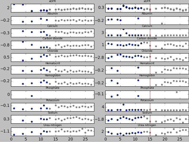
Figure 5: Monthly average lab values for two patients. The left pane show the lab data for a patient who doesn’t initiate dialysis or undergo a kidney transplant. The right pane shows a patient that starts dialysis in the outcome window. The vertical red line shows when that patient starts dialysis. The x-axis is the number of months from the beginning of the training window and the y-axis is the standardized lab value.

Figure 5 in the Supplementary Materials shows an example of lab data for a patient that does not start dialysis or undergo a kidney transplant in the outcome window and for a patient the starts dialysis in the outcome window.

We compared the performance of the CNN2 architecture adapted to this prediction task to two logistic regression baselines and a random forest. Additional details are provided in the Supplementary Materials.

6.2 Results

The 4 models achieved similar performance on this prediction task (see Table 4). The small sample size and the single binary outcome distinguish this task from the multi-disease setting and may make it difficult to observe large differences in performance between the models. A small number of features also seem to account for much of the signal. We observed that a logistic regression with a large L1 penalty achieves good performance on the task despite only using eGFR, urea nitrogen, age and gender as features.

7 Conclusion

In this work, we presented a large-scale application of two novel convolutional neural network architectures and a LSTM recurrent neural network for the task of multi-task early disease onset detection. These representation-based approaches significantly outperform a logistic regression with several hand-engineered, clinically relevant features. Interestingly, in our earlier work, we found that despite the large amount of missing data in the setting considered, preprocessing the data by imputing missing values did not significantly improve results (Razavian and Sontag, 2015). As medical home and consumer healthcare technologies rapidly progress, we envision a growing role for automatic risk stratification of patients based solely on raw physiological and chemical signals.

AcknowledgmentsThe authors gratefully acknowledge support by Independence Blue Cross. The Tesla K40s used for this research were donated by the NVIDIA Corporation. We thank Dr. Yindalon Aphinyanaphongs, Dr. Steven Horng, and Dr. Saul Blecker for providing helpful clinical perspectives throughout this research.

8 Supplementary Materials
for Multi-task Prediction of Disease Onsets from Longitudinal Lab Tests

8.1 Cross-validation results

For the convolutional models, we set the number of filters to be 64 for all the convolution layers with a kernel length of 8 (months) and a step size of 1. Each max-pooling module had a horizontal length of 3 and vertical length of 1 with a step size of 3 in the horizontal direction (i.e. no overlap). Each convolution module was followed by a batch normalization module (Ioffe and Szegedy (2015)) and then a ReLU nonlinearity (Nair and Hinton (2010)). We had 2 fully connected layers (with 100 nodes each, cross validated over [30,50, 100, 500,1000]) after concatenating the outputs of all the convolution layers. Each of the fully connected layers were followed by a batch normalization layer and a ReLU nonlinearity layer. We also added one Dropout module (Srivastava et al. (2014)) (0.5 dropout probability) before each fully connected layer. We tested models with and without batch-normalization and found that the networks converge much faster with batch-normalization.

We had the following layers after the last ReLu nonlinearity for each of the 171 diseases: a Dropout layer(0.5 dropout probability), a fully connected layer (of size 2 nodes corresponding to binary outcome), a batch normalization layer and a Log Softmax Layer. A learning rate of $0.1$ was selected from among the values $[0.001,0.01,0.05,0.1,1]$ using the validation set average AUC (over all diseases) after 10 epochs. Training was done using Adadelta(Zeiler (2012)) optimization, which is a variant of stochastic gradient descent with adaptive step size. We used mini-batches of size 256.

For the LSTM network, we cross-validated over the hidden LSTM units ([100 500 1000]), and 500 was selected as the best. For the shared part of the network, we used the best parameters found for the convolution models.

8.2 Model details for CKD Case Study

We compared the following models:

• CNN2. We applied the CNN2 architecture used in the multi-disease prediction task with 8 filters with kernel dimensions of 8x1. We used the raw clinical and demographic data as input without additional feature engineering. We chose the learning rate and the architecture based on cross-validation using random sampling of hyperparameters (Bergstra and Bengio (2012)).

• L2-regularized, logistic regression. For each lab, we added one feature for the average lab value across the training window. We included gender and the diagnosis and prescription data as binary indicators and age as a continuous variable. We chose a regularization constant based on cross-validation.

• L1-regularized, logistic regression. For each lab, we added features to the regression for the average lab value for the patient over the last 3 months of the training window, the past 6 months of the training window and over the entire training window. We also added binary features for whether or not the lab increased, decreased or fluctuated over the last 3 months, 6 months and over the entire training window. We included gender and the diagnosis and prescription data as binary indicators and age as a continuous variable. We chose a regularization constant based on cross-validation.

• Random forests. We used the raw clinical and demographic data as input without additional feature engineering. We chose the number of trees in the forest, the maximum depth of each tree, the maximum number of features to consider when looking for the best split, the minimum number of samples required to split a node, and the minimum number of samples in newly created leaves based on cross-validation using random sampling of hyperparameters.

8.3 Figures and Tables

Table 2: Name and LOINC of labs included as features for multi-task prediction

Lab name	LOINC
Creatinine	2160-0
Urea nitrogen	3094-0
Potassium	2823-3
Glucose	2345-7
Alanine aminotransferase	1742-6
Aspartate aminotransferase	1920-8
Protein	2885-2
Albumin	1751-7
Cholesterol	2093-3
Triglyceride	2571-8
Cholesterol.in LDL	13457-7
Calcium	17861-6
Sodium	2951-2
Chloride	2075-0
Carbon dioxide	2028-9
Urea nitrogen/Creatinine	3097-3
Bilirubin	1975-2
Albumin/Globulin	1759-0

Table 3: Clinical features included in predictive models in the CKD case study

Type	Description
Lab	33914-3 eGFR/1.73 sq M [Volume Rate/Area] in Serum or Plasma
Lab	48642-3 eGFR/​1.73 sq M among non-blacks [Volume Rate/​Area] in Serum or Plasma
Lab	48643-1 eGFR/​1.73 sq M among blacks [Volume Rate/​Area] in Serum or Plasma
Lab	2160-0 Creatinine [Mass/​volume] in Serum or Plasma
Lab	1751-7 Albumin [Mass/​volume] in Serum or Plasma
Lab	17861-6 Calcium [Mass/​volume] in Serum or Plasma
Lab	2028-9 Carbon dioxide, total [Moles/​volume] in Serum or Plasma
Lab	9318-7 Albumin/​Creatinine [Mass Ratio] in Urine
Lab	2777-1 Phosphate [Mass/​volume] in Serum or Plasma
Lab	3094-0 Urea nitrogen [Mass/​volume] in Serum or Plasma
Lab	2075-0 Chloride [Moles/​volume] in Serum or Plasma
Lab	4544-3 Hematocrit [Volume Fraction] of Blood by Automated count
Lab	718-7 Hemoglobin [Mass/​volume] in Blood
Lab	2823-3 Potassium [Moles/​volume] in Serum or Plasma
Drug class	BETA-ADRENERGIC BLOCKING AGENTS
Drug class	LOOP DIURETICS
Drug class	HMG-COA REDUCTASE INHIBITORS
Drug class	DIHYDROPYRIDINES
Drug class	ANGIOTENSIN-CONVERTING ENZYME INHIBITORS
Drug class	ANGIOTENSIN II RECEPTOR ANTAGONISTS
Drug class	VITAMIN D
Drug class	DIRECT VASODILATORS
Drug class	THIAZIDE DIURETICS
Drug class	CHOLESTEROL ABSORPTION INHIBITORS
Drug class	THIAZIDE-LIKE DIURETICS
Drug class	PHOSPHATE-REMOVING AGENTS
Drug class	CENTRAL ALPHA-AGONISTS
Drug class	HEMATOPOIETIC AGENTS
Drug class	ALPHA-ADRENERGIC BLOCKING AGENTS
Diagnosis	403.11 Ben hyp kid w cr kid V
Diagnosis	403.91 Hyp kid NOS w cr kid V
Diagnosis	285.21 Anemia in chr kidney dis
Diagnosis	588.81 Sec hyperparathyrd-renal
Diagnosis	V72.81 Preop cardiovsclr exam
Diagnosis	786.50 Chest pain NOS
Diagnosis	600.00 BPH w/o urinary obs/LUTS
Diagnosis	244.9 Hypothyroidism NOS
Diagnosis	599.0 Urin tract infection NOS
Diagnosis	250.02 DMII wo cmp uncntrld
Diagnosis	250.01 DMI wo cmp nt st uncntrl
Diagnosis	530.81 Esophageal reflux
Diagnosis	V58.61 Long-term use anticoagul
Diagnosis	780.79 Malaise and fatigue NEC
Diagnosis	562.10 Dvrtclo colon w/o hmrhg

Table 4: Area Under ROC curve for comparing the held out test score

	AUC
CNN2	0.774
Random forest	0.774
L1-regularized logistic regression with hand-engineered features	0.768
L2-regularized logistic regression	0.755

Table 5: Top Features from the baseline model for 585.6 End stage renal disease

Feature	weight	Feature	weight
Glucose(2345-7) -decreasing	-1.099	Alanine(1742-6) -increasing	0.2263
Chloride(2075-0) -latest value	0.4988	Cholesterol.in(13457-7) -increasing	-0.216
Glucose(2345-7) -latest value	-0.485	Urea(3094-0) -maximum	-0.214
Creatinine(2160-0) -maximum	0.4837	Aspartate(1920-8) -maximum	0.2016
Carbon(2028-9) -increasing	0.4500	Sodium(2951-2) -latest value	-0.191
Cholesterol.in(13457-7) -minimum	0.3037	Creatinine(2160-0) -decreasing	0.1918
Cholesterol.in(13457-7) -latest value	-0.254	Chloride(2075-0) -maximum	-0.177
Glucose(2345-7) -minimum	-0.251	Carbon(2028-9) -minimum	-0.170
Calcium(17861-6) -decreasing	-0.239	Alanine(1742-6) -minimum	-0.122
Urea(3094-0) -increasing	0.2344	Protein(2885-2) -increasing	0.1208

Table 6: Top Features from the baseline model for 285.21 Anemia in chr kidney dis

Feature	weight	Feature	weight
Chloride(2075-0) -latest value	0.7909	Calcium(17861-6) -maximum	-0.305
Cholesterol.in(13457-7) -minimum	0.7244	Triglyceride(2571-8) -decreasing	-0.301
Glucose(2345-7) -decreasing	-0.717	Triglyceride(2571-8) -increasing	-0.300
Creatinine(2160-0) -maximum	0.5596	Carbon(2028-9) -maximum	-0.291
Creatinine(2160-0) -minimum	0.4692	Cholesterol.in(13457-7) -increasing	-0.290
Chloride(2075-0) -increasing	-0.442	Alanine(1742-6) -minimum	-0.284
Potassium(2823-3) -increasing	-0.381	Glucose(2345-7) -latest value	-0.273
Cholesterol.in(13457-7) -latest value	-0.370	Alanine(1742-6) -increasing	0.2531
Aspartate(1920-8) -decreasing	0.3658	Carbon(2028-9) -increasing	0.2383
Glucose(2345-7) -minimum	-0.324	Urea(3094-0) -increasing	0.2359

Table 7: Top Features from the baseline model for 585.3 Chr kidney dis stage III

Feature	weight	Feature	weight
Glucose(2345-7) -decreasing	-0.749	Triglyceride(2571-8) -maximum	0.2169
Cholesterol.in(13457-7) -minimum	0.6567	Alanine(1742-6) -maximum	0.2060
Chloride(2075-0) -latest value	0.5660	Cholesterol.in(13457-7) -increasing	-0.200
Triglyceride(2571-8) -increasing	-0.425	Potassium(2823-3) -decreasing	0.1638
Creatinine(2160-0) -maximum	0.4086	Carbon(2028-9) -increasing	0.1509
Cholesterol.in(13457-7) -latest value	-0.374	Alanine(1742-6) -minimum	-0.143
Chloride(2075-0) -maximum	-0.361	Glucose(2345-7) -minimum	-0.140
Creatinine(2160-0) -minimum	0.3368	Calcium(17861-6) -increasing	0.1407
Glucose(2345-7) -latest value	-0.286	Albumin(1751-7) -minimum	0.1385
Alanine(1742-6) -increasing	0.2667	Potassium(2823-3) -minimum	-0.137

Table 8: Top Features from the baseline model for 584.9 Acute kidney failure NOS

Feature	weight	Feature	weight
Glucose(2345-7) -decreasing	-0.729	Carbon(2028-9) -increasing	0.1915
Creatinine(2160-0) -minimum	0.3994	Alanine(1742-6) -minimum	-0.180
Glucose(2345-7) -latest value	-0.388	Alanine(1742-6) -increasing	0.1694
Cholesterol.in(13457-7) -latest value	-0.372	Triglyceride(2571-8) -increasing	-0.156
Creatinine(2160-0) -maximum	0.3195	Glucose(2345-7) -maximum	0.1402
Chloride(2075-0) -latest value	0.3087	Potassium(2823-3) -minimum	-0.136
Creatinine(2160-0) -decreasing	0.2750	Chloride(2075-0) -increasing	-0.129
Cholesterol.in(13457-7) -minimum	0.2571	Aspartate(1920-8) -latest value	0.1212
Urea(3094-0) -increasing	0.2374	Potassium(2823-3) -latest value	0.1078
Albumin(1751-7) -maximum	0.2309	Cholesterol.in(13457-7) -increasing	-0.105

Table 9: Top Features from the baseline model for 250.01 DMI wo cmp nt st uncntrl

Feature	weight	Feature	weight
Alanine(1742-6) -minimum	-0.683	Creatinine(2160-0) -minimum	0.1255
Creatinine(2160-0) -decreasing	0.6438	Bilirubin(1975-2) -maximum	0.1244
Glucose(2345-7) -decreasing	-0.235	Aspartate(1920-8) -increasing	-0.116
Glucose(2345-7) -minimum	-0.227	Cholesterol(2093-3) -latest value	0.1157
Urea(3094-0) -decreasing	0.2204	Alanine(1742-6) -decreasing	-0.092
Sodium(2951-2) -increasing	0.1755	Urea(3097-3) -latest value	-0.078
Urea(3094-0) -increasing	-0.172	Protein(2885-2) -minimum	0.0750
Protein(2885-2) -increasing	0.1526	Protein(2885-2) -decreasing	-0.072
Albumin(1751-7) -maximum	0.1274	Alanine(1742-6) -latest value	0.0699
Alanine(1742-6) -maximum	-0.126	Cholesterol.in(13457-7) -increasing	0.0661

Table 10: Top Features from the baseline model for 250.02 DMII wo cmp uncntrld

Feature	weight	Feature	weight
Alanine(1742-6) -minimum	-0.727	Urea(3094-0) -minimum	-0.165
Creatinine(2160-0) -decreasing	0.6069	Aspartate(1920-8) -maximum	0.1647
Cholesterol(2093-3) -latest value	0.3880	Albumin(1751-7) -maximum	0.1594
Sodium(2951-2) -increasing	0.3318	Protein(2885-2) -increasing	0.1521
Alanine(1742-6) -increasing	-0.330	Calcium(17861-6) -increasing	-0.146
Urea(3094-0) -decreasing	0.2875	Triglyceride(2571-8) -increasing	-0.145
Glucose(2345-7) -maximum	0.2016	Albumin(1751-7) -minimum	0.1437
Potassium(2823-3) -latest value	-0.184	Cholesterol.in(13457-7) -minimum	0.1392
Glucose(2345-7) -decreasing	-0.182	Creatinine(2160-0) -latest value	-0.136
Aspartate(1920-8) -decreasing	-0.168	Alanine(1742-6) -maximum	-0.136

Table 11: Top Features from the baseline model for 593.9 Renal and ureteral dis NOS

Feature	weight	Feature	weight
Glucose(2345-7) -decreasing	-0.769	Urea(3094-0) -maximum	-0.171
Chloride(2075-0) -latest value	0.5136	Cholesterol.in(13457-7) -increasing	-0.150
Cholesterol.in(13457-7) -minimum	0.4754	Calcium(17861-6) -decreasing	0.1446
Cholesterol.in(13457-7) -latest value	-0.345	Alanine(1742-6) -decreasing	-0.143
Alanine(1742-6) -maximum	0.2568	Sodium(2951-2) -decreasing	-0.142
Creatinine(2160-0) -maximum	0.2394	Carbon(2028-9) -minimum	-0.137
Creatinine(2160-0) -minimum	0.2163	Cholesterol.in(13457-7) -decreasing	-0.133
Creatinine(2160-0) -decreasing	0.2093	Carbon(2028-9) -increasing	0.1204
Calcium(17861-6) -maximum	-0.182	Albumin(1751-7) -maximum	0.1146
Glucose(2345-7) -maximum	0.1816	Alanine(1742-6) -minimum	-0.113

Table 12: Top Features from the baseline model for 428.0 CHF NOS

Feature	weight	Feature	weight
Glucose(2345-7) -decreasing	-0.449	Alanine(1742-6) -increasing	0.1467
Glucose(2345-7) -maximum	0.2493	Chloride(2075-0) -decreasing	-0.146
Cholesterol.in(13457-7) -minimum	0.2140	Creatinine(2160-0) -maximum	0.1251
Creatinine(2160-0) -decreasing	0.2126	Alanine(1742-6) -minimum	-0.124
Albumin(1751-7) -maximum	0.2045	Creatinine(2160-0) -latest value	-0.120
Chloride(2075-0) -latest value	0.1996	Albumin(1751-7) -latest value	-0.112
Glucose(2345-7) -latest value	-0.195	Aspartate(1920-8) -decreasing	0.1106
Creatinine(2160-0) -minimum	0.1911	Cholesterol(2093-3) -decreasing	-0.100
Calcium(17861-6) -decreasing	0.1588	Alanine(1742-6) -decreasing	0.1000
Cholesterol.in(13457-7) -maximum	-0.156	Alanine(1742-6) -latest value	-0.098

Table 13: Top Features from the baseline model for V05.3 Need prphyl vc vrl hepat

Feature	weight	Feature	weight
Carbon(2028-9) -increasing	0.4567	Sodium(2951-2) -latest value	0.0
Creatinine(2160-0) -maximum	0.4441	Sodium(2951-2) -decreasing	0.0
Glucose(2345-7) -decreasing	-0.233	Sodium(2951-2) -increasing	0.0
Aspartate(1920-8) -decreasing	0.1593	Sodium(2951-2) -minimum	0.0
Creatinine(2160-0) -minimum	-0.119	Calcium(17861-6) -decreasing	0.0
Urea(3094-0) -minimum	-0.109	Calcium(17861-6) -latest value	0.0
Creatinine(2160-0) -increasing	-0.058	Calcium(17861-6) -increasing	0.0
Protein(2885-2) -maximum	0.0177	Calcium(17861-6) -minimum	0.0
Alanine(1742-6) -maximum	0.0164	Calcium(17861-6) -maximum	0.0
Chloride(2075-0) -maximum	0.0	Cholesterol.in(13457-7) -latest value	0.0

Table 14: Top Features from the baseline model for 790.93 Elvtd prstate spcf antgn

Feature	weight	Feature	weight
Alanine(1742-6) -maximum	0.2819	Triglyceride(2571-8) -minimum	0.1261
Potassium(2823-3) -minimum	0.2446	Alanine(1742-6) -increasing	-0.120
Sodium(2951-2) -latest value	0.2335	Protein(2885-2) -increasing	-0.115
Cholesterol.in(13457-7) -minimum	0.2137	Triglyceride(2571-8) -increasing	-0.096
Creatinine(2160-0) -decreasing	-0.179	Alanine(1742-6) -decreasing	0.0861
Cholesterol(2093-3) -latest value	0.1770	Sodium(2951-2) -increasing	0.0832
Potassium(2823-3) -increasing	-0.146	Urea(3097-3) -latest value	0.0789
Glucose(2345-7) -minimum	0.1437	Potassium(2823-3) -decreasing	-0.076
Cholesterol(2093-3) -maximum	-0.138	Albumin(1751-7) -decreasing	-0.073
Cholesterol(2093-3) -increasing	0.1277	Cholesterol(2093-3) -minimum	-0.070

Table 15: Top Features from the baseline model for 185. Malign neopl prostate

Feature	weight	Feature	weight
Cholesterol(2093-3) -minimum	-0.293	Cholesterol(2093-3) -latest value	0.1599
Aspartate(1920-8) -maximum	0.2527	Sodium(2951-2) -decreasing	0.1498
Alanine(1742-6) -latest value	0.2005	Cholesterol(2093-3) -maximum	-0.144
Glucose(2345-7) -decreasing	-0.188	Triglyceride(2571-8) -minimum	0.1375
Cholesterol.in(13457-7) -minimum	0.1791	Cholesterol(2093-3) -increasing	0.1334
Aspartate(1920-8) -decreasing	-0.174	Alanine(1742-6) -decreasing	-0.130
Alanine(1742-6) -increasing	-0.173	Potassium(2823-3) -minimum	0.1305
Potassium(2823-3) -decreasing	-0.168	Potassium(2823-3) -maximum	0.1143
Alanine(1742-6) -maximum	0.1676	Urea(3094-0) -maximum	-0.110
Sodium(2951-2) -increasing	0.1648	Bilirubin(1975-2) -decreasing	-0.108

Table 16: Top Features from the baseline model for 274.9 Gout NOS

Feature	weight	Feature	weight
Glucose(2345-7) -decreasing	-0.414	Creatinine(2160-0) -decreasing	0.1201
Cholesterol.in(13457-7) -latest value	-0.266	Urea(3094-0) -increasing	0.1181
Aspartate(1920-8) -increasing	-0.261	Carbon(2028-9) -increasing	0.1005
Cholesterol.in(13457-7) -minimum	0.2584	Aspartate(1920-8) -maximum	0.0980
Creatinine(2160-0) -maximum	0.2092	Protein(2885-2) -decreasing	-0.096
Glucose(2345-7) -latest value	-0.200	Chloride(2075-0) -latest value	0.0953
Glucose(2345-7) -increasing	-0.194	Creatinine(2160-0) -minimum	0.0881
Urea(3094-0) -minimum	0.1545	Creatinine(2160-0) -latest value	-0.086
Alanine(1742-6) -maximum	0.1316	Aspartate(1920-8) -latest value	-0.078
Protein(2885-2) -latest value	0.1295	Cholesterol(2093-3) -increasing	-0.077

Table 17: Top Features from the baseline model for 362.52 Exudative macular degen

Feature	weight	Feature	weight
Creatinine(2160-0) -maximum	0.3761	Glucose(2345-7) -decreasing	0.1683
Creatinine(2160-0) -latest value	-0.270	Creatinine(2160-0) -minimum	0.1545
Alanine(1742-6) -latest value	-0.254	Cholesterol.in(13457-7) -increasing	0.1477
Urea(3094-0) -increasing	-0.241	Albumin(1751-7) -latest value	-0.145
Alanine(1742-6) -increasing	0.2399	Potassium(2823-3) -latest value	0.1365
Alanine(1742-6) -minimum	0.2304	Aspartate(1920-8) -increasing	-0.120
Glucose(2345-7) -latest value	-0.200	Calcium(17861-6) -decreasing	0.1134
Potassium(2823-3) -minimum	0.1818	Glucose(2345-7) -minimum	0.0982
Cholesterol.in(13457-7) -latest value	0.1795	Aspartate(1920-8) -minimum	0.0966
Urea(3094-0) -maximum	-0.168	Carbon(2028-9) -increasing	-0.090

Table 18: Top Features from the baseline model for 607.84 Impotence, organic orign

Feature	weight	Feature	weight
Cholesterol(2093-3) -minimum	-0.296	Urea(3094-0) -increasing	-0.140
Alanine(1742-6) -maximum	0.2400	Glucose(2345-7) -latest value	0.1306
Alanine(1742-6) -increasing	-0.237	Aspartate(1920-8) -decreasing	-0.116
Aspartate(1920-8) -increasing	-0.210	Urea(3094-0) -minimum	-0.111
Potassium(2823-3) -increasing	0.1967	Protein(2885-2) -maximum	0.1038
Potassium(2823-3) -decreasing	0.1671	Chloride(2075-0) -minimum	0.0963
Creatinine(2160-0) -maximum	-0.160	Cholesterol.in(13457-7) -minimum	0.0905
Protein(2885-2) -latest value	-0.153	Creatinine(2160-0) -increasing	-0.086
Creatinine(2160-0) -decreasing	0.1531	Aspartate(1920-8) -latest value	0.0856
Calcium(17861-6) -latest value	-0.141	Alanine(1742-6) -decreasing	-0.078

Table 19: Top Features from the baseline model for 511.9 Pleural effusion NOS

Feature	weight	Feature	weight
Alanine(1742-6) -increasing	0.4040	Triglyceride(2571-8) -increasing	-0.194
Glucose(2345-7) -decreasing	-0.366	Creatinine(2160-0) -maximum	0.1678
Urea(3094-0) -latest value	-0.297	Aspartate(1920-8) -increasing	-0.166
Chloride(2075-0) -latest value	0.2698	Cholesterol.in(13457-7) -decreasing	-0.158
Urea(3094-0) -increasing	0.2680	Glucose(2345-7) -latest value	-0.154
Chloride(2075-0) -maximum	-0.251	Cholesterol(2093-3) -decreasing	-0.154
Aspartate(1920-8) -latest value	0.2400	Creatinine(2160-0) -latest value	0.1370
Cholesterol.in(13457-7) -minimum	0.2396	Cholesterol.in(13457-7) -maximum	-0.135
Alanine(1742-6) -minimum	-0.223	Albumin(1751-7) -maximum	0.1317
Alanine(1742-6) -maximum	-0.200	Triglyceride(2571-8) -maximum	-0.129

Table 20: Top Features from the baseline model for 616.10 Vaginitis NOS

Feature	weight	Feature	weight
Alanine(1742-6) -maximum	-0.567	Cholesterol(2093-3) -maximum	0.1796
Protein(2885-2) -decreasing	-0.386	Creatinine(2160-0) -maximum	-0.172
Alanine(1742-6) -increasing	0.3732	Cholesterol.in(13457-7) -minimum	-0.151
Creatinine(2160-0) -increasing	-0.340	Calcium(17861-6) -decreasing	0.1461
Calcium(17861-6) -maximum	0.2638	Triglyceride(2571-8) -increasing	0.0902
Urea(3094-0) -latest value	-0.263	Bilirubin(1975-2) -minimum	-0.075
Creatinine(2160-0) -minimum	-0.230	Albumin/Globulin(1759-0) -increasing	0.0708
Protein(2885-2) -minimum	-0.200	Urea(3094-0) -increasing	-0.067
Cholesterol.in(13457-7) -latest value	0.1909	Glucose(2345-7) -decreasing	0.0619
Glucose(2345-7) -minimum	-0.190	Potassium(2823-3) -decreasing	-0.058

Table 21: Top Features from the baseline model for 600.01 BPH w urinary obs/LUTS

Feature	weight	Feature	weight
Glucose(2345-7) -decreasing	-0.358	Sodium(2951-2) -latest value	0.1253
Alanine(1742-6) -increasing	-0.324	Chloride(2075-0) -latest value	0.1236
Creatinine(2160-0) -latest value	-0.255	Cholesterol.in(13457-7) -decreasing	-0.114
Protein(2885-2) -latest value	-0.253	Aspartate(1920-8) -increasing	-0.100
Sodium(2951-2) -decreasing	0.2298	Creatinine(2160-0) -decreasing	0.0918
Cholesterol.in(13457-7) -minimum	0.1959	Cholesterol.in(13457-7) -latest value	-0.091
Aspartate(1920-8) -maximum	0.1736	Chloride(2075-0) -increasing	-0.083
Glucose(2345-7) -increasing	-0.134	Urea(3094-0) -maximum	-0.076
Creatinine(2160-0) -maximum	-0.133	Potassium(2823-3) -increasing	-0.072
Urea(3094-0) -latest value	0.1271	Chloride(2075-0) -decreasing	-0.071

Table 22: Top Features from the baseline model for 285.29 Anemia-other chronic dis

Feature	weight	Feature	weight
Glucose(2345-7) -decreasing	-0.492	Triglyceride(2571-8) -increasing	-0.205
Creatinine(2160-0) -increasing	0.3508	Urea(3094-0) -maximum	-0.189
Protein(2885-2) -latest value	0.3098	Albumin(1751-7) -maximum	0.1885
Aspartate(1920-8) -decreasing	0.3042	Aspartate(1920-8) -maximum	-0.183
Carbon(2028-9) -increasing	0.2610	Chloride(2075-0) -latest value	0.1796
Creatinine(2160-0) -maximum	0.2594	Potassium(2823-3) -latest value	-0.168
Alanine(1742-6) -increasing	0.2468	Aspartate(1920-8) -latest value	0.1632
Creatinine(2160-0) -minimum	0.2386	Creatinine(2160-0) -decreasing	0.1492
Potassium(2823-3) -minimum	0.2368	Cholesterol.in(13457-7) -decreasing	-0.147
Cholesterol.in(13457-7) -increasing	-0.216	Cholesterol(2093-3) -latest value	-0.134

Table 23: Top Features from the baseline model for 346.90 Migrne unsp wo ntrc mgrn

Feature	weight	Feature	weight
Cholesterol.in(13457-7) -minimum	-0.403	Aspartate(1920-8) -maximum	-0.105
Cholesterol(2093-3) -increasing	0.3081	Alanine(1742-6) -latest value	-0.102
Cholesterol.in(13457-7) -latest value	0.2965	Creatinine(2160-0) -increasing	-0.096
Alanine(1742-6) -minimum	0.2748	Protein(2885-2) -decreasing	0.0964
Sodium(2951-2) -decreasing	-0.204	Sodium(2951-2) -minimum	0.0925
Cholesterol.in(13457-7) -decreasing	0.1985	Potassium(2823-3) -latest value	-0.088
Aspartate(1920-8) -increasing	0.1974	Potassium(2823-3) -decreasing	-0.084
Albumin/Globulin(1759-0) -increasing	0.1783	Carbon(2028-9) -maximum	0.0836
Glucose(2345-7) -latest value	-0.132	Albumin/Globulin(1759-0) -maximum	0.0587
Protein(2885-2) -maximum	0.1100	Calcium(17861-6) -decreasing	0.0528

Table 24: Top Features from the baseline model for 427.31 Atrial fibrillation

Feature	weight	Feature	weight
Creatinine(2160-0) -maximum	0.2260	Albumin/Globulin(1759-0) -latest value	-0.019
Alanine(1742-6) -increasing	0.1981	Creatinine(2160-0) -latest value	-0.015
Glucose(2345-7) -maximum	0.1956	Urea(3097-3) -latest value	-0.011
Glucose(2345-7) -latest value	-0.099	Sodium(2951-2) -decreasing	0.0089
Urea(3094-0) -maximum	-0.089	Creatinine(2160-0) -minimum	0.0084
Urea(3094-0) -latest value	-0.082	Cholesterol.in(13457-7) -latest value	-0.007
Glucose(2345-7) -decreasing	-0.079	Cholesterol(2093-3) -decreasing	-0.000
Alanine(1742-6) -minimum	-0.066	Potassium(2823-3) -minimum	0.0
Urea(3094-0) -minimum	-0.037	Chloride(2075-0) -minimum	0.0
Cholesterol(2093-3) -increasing	-0.031	Chloride(2075-0) -maximum	0.0

Table 25: Top Features from the baseline model for 250.00 DMII wo cmp nt st uncntr

Feature	weight	Feature	weight
Alanine(1742-6) -minimum	-0.406	Sodium(2951-2) -maximum	-0.104
Aspartate(1920-8) -increasing	-0.371	Potassium(2823-3) -latest value	-0.099
Creatinine(2160-0) -decreasing	0.2839	Urea(3097-3) -maximum	0.0990
Albumin(1751-7) -maximum	0.2038	Triglyceride(2571-8) -maximum	0.0983
Alanine(1742-6) -increasing	-0.184	Urea(3094-0) -decreasing	0.0894
Glucose(2345-7) -maximum	0.1364	Cholesterol.in(13457-7) -minimum	0.0803
Aspartate(1920-8) -maximum	0.1264	Chloride(2075-0) -increasing	-0.075
Cholesterol.in(13457-7) -latest value	0.1119	Aspartate(1920-8) -minimum	0.0737
Calcium(17861-6) -increasing	-0.107	Glucose(2345-7) -increasing	0.0639
Glucose(2345-7) -decreasing	-0.105	Bilirubin(1975-2) -increasing	-0.060

Table 26: Top Features from the baseline model for 425.4 Prim cardiomyopathy NEC

Feature	weight	Feature	weight
Glucose(2345-7) -decreasing	-0.272	Urea(3094-0) -increasing	-0.010
Creatinine(2160-0) -maximum	0.1168	Protein(2885-2) -latest value	0.0038
Albumin(1751-7) -maximum	0.1132	Sodium(2951-2) -latest value	0.0
Urea(3094-0) -latest value	-0.070	Chloride(2075-0) -maximum	0.0
Creatinine(2160-0) -minimum	0.0647	Chloride(2075-0) -minimum	0.0
Creatinine(2160-0) -decreasing	0.0560	Sodium(2951-2) -decreasing	0.0
Urea(3094-0) -maximum	-0.025	Sodium(2951-2) -increasing	0.0
Glucose(2345-7) -maximum	0.0167	Sodium(2951-2) -maximum	0.0
Aspartate(1920-8) -maximum	0.0165	Chloride(2075-0) -increasing	0.0
Glucose(2345-7) -latest value	-0.014	Calcium(17861-6) -latest value	0.0

Table 27: Top Features from the baseline model for 728.87 Muscle weakness-general

Feature	weight	Feature	weight
Alanine(1742-6) -increasing	0.2943	Glucose(2345-7) -latest value	-0.087
Creatinine(2160-0) -minimum	0.2361	Calcium(17861-6) -latest value	-0.083
Glucose(2345-7) -decreasing	-0.189	Calcium(17861-6) -maximum	-0.079
Creatinine(2160-0) -decreasing	0.1719	Urea(3094-0) -latest value	-0.076
Creatinine(2160-0) -increasing	0.1644	Alanine(1742-6) -maximum	-0.075
Creatinine(2160-0) -maximum	0.1479	Alanine(1742-6) -latest value	-0.071
Alanine(1742-6) -minimum	-0.112	Albumin(1751-7) -minimum	0.0697
Triglyceride(2571-8) -maximum	-0.108	Cholesterol.in(13457-7) -increasing	-0.067
Urea(3094-0) -minimum	0.1040	Protein(2885-2) -decreasing	-0.064
Aspartate(1920-8) -minimum	0.1020	Protein(2885-2) -increasing	0.0623

Table 28: Top Features from the baseline model for 620.2 Ovarian cyst NEC/NOS

Feature	weight	Feature	weight
Alanine(1742-6) -decreasing	0.5072	Protein(2885-2) -decreasing	0.1532
Cholesterol.in(13457-7) -minimum	-0.287	Urea(3094-0) -minimum	-0.147
Aspartate(1920-8) -decreasing	-0.285	Cholesterol.in(13457-7) -increasing	-0.136
Alanine(1742-6) -latest value	-0.232	Alanine(1742-6) -maximum	-0.131
Urea(3094-0) -decreasing	-0.213	Glucose(2345-7) -decreasing	0.1079
Creatinine(2160-0) -latest value	0.2003	Aspartate(1920-8) -latest value	0.1043
Chloride(2075-0) -maximum	0.1717	Glucose(2345-7) -minimum	0.1004
Urea(3094-0) -maximum	0.1681	Albumin(1751-7) -maximum	0.0953
Creatinine(2160-0) -maximum	-0.157	Urea(3097-3) -latest value	0.0884
Glucose(2345-7) -increasing	-0.156	Albumin(1751-7) -latest value	0.0792

Table 29: Top Features from the baseline model for 286.9 Coagulat defect NEC/NOS

Feature	weight	Feature	weight
Chloride(2075-0) -minimum	-0.337	Creatinine(2160-0) -maximum	0.1148
Carbon(2028-9) -increasing	0.3219	Glucose(2345-7) -maximum	0.1124
Glucose(2345-7) -decreasing	-0.300	Creatinine(2160-0) -latest value	0.1008
Creatinine(2160-0) -minimum	0.2578	Aspartate(1920-8) -decreasing	0.0993
Triglyceride(2571-8) -increasing	-0.203	Albumin(1751-7) -latest value	-0.090
Albumin(1751-7) -maximum	0.1802	Creatinine(2160-0) -increasing	0.0865
Alanine(1742-6) -minimum	-0.179	Sodium(2951-2) -maximum	-0.082
Cholesterol(2093-3) -latest value	-0.147	Urea(3097-3) -latest value	-0.080
Protein(2885-2) -decreasing	-0.139	Alanine(1742-6) -increasing	0.0764
Triglyceride(2571-8) -latest value	-0.123	Potassium(2823-3) -latest value	-0.075

Table 30: Top Features from the baseline model for 443.9 Periph vascular dis NOS

Feature	weight	Feature	weight
Glucose(2345-7) -decreasing	-0.395	Creatinine(2160-0) -maximum	0.1184
Alanine(1742-6) -increasing	0.2594	Triglyceride(2571-8) -minimum	0.1182
Alanine(1742-6) -minimum	-0.227	Triglyceride(2571-8) -increasing	-0.116
Cholesterol.in(13457-7) -latest value	-0.199	Sodium(2951-2) -increasing	0.1053
Aspartate(1920-8) -latest value	0.1825	Chloride(2075-0) -minimum	-0.095
Creatinine(2160-0) -minimum	0.1554	Urea(3094-0) -increasing	0.0914
Glucose(2345-7) -maximum	0.1403	Albumin/Globulin(1759-0) -maximum	-0.077
Protein(2885-2) -decreasing	-0.133	Aspartate(1920-8) -increasing	-0.075
Urea(3094-0) -latest value	-0.128	Aspartate(1920-8) -minimum	0.0724
Glucose(2345-7) -minimum	-0.123	Cholesterol.in(13457-7) -decreasing	-0.065

Table 31: Top Features from the baseline model for 362.51 Nonexudat macular degen

Feature	weight	Feature	weight
Creatinine(2160-0) -latest value	-0.117	Sodium(2951-2) -decreasing	0.0
Glucose(2345-7) -decreasing	-0.080	Sodium(2951-2) -increasing	0.0
Protein(2885-2) -latest value	-0.060	Sodium(2951-2) -minimum	0.0
Creatinine(2160-0) -increasing	0.0179	Sodium(2951-2) -maximum	0.0
Glucose(2345-7) -latest value	-0.015	Calcium(17861-6) -decreasing	0.0
Creatinine(2160-0) -maximum	0.0099	Chloride(2075-0) -minimum	0.0
Glucose(2345-7) -minimum	0.0075	Calcium(17861-6) -increasing	0.0
Urea(3094-0) -latest value	-0.001	Calcium(17861-6) -minimum	0.0
Chloride(2075-0) -maximum	0.0	Calcium(17861-6) -maximum	0.0
Sodium(2951-2) -latest value	0.0	Cholesterol.in(13457-7) -latest value	0.0

Table 32: Top Features from the baseline model for 414.9 Chr ischemic hrt dis NOS

Feature	weight	Feature	weight
Glucose(2345-7) -decreasing	-0.328	Chloride(2075-0) -latest value	0.1241
Glucose(2345-7) -maximum	0.2678	Alanine(1742-6) -minimum	-0.116
Aspartate(1920-8) -increasing	-0.264	Sodium(2951-2) -increasing	0.1142
Cholesterol.in(13457-7) -latest value	-0.229	Cholesterol.in(13457-7) -increasing	-0.108
Creatinine(2160-0) -decreasing	0.1837	Cholesterol(2093-3) -minimum	-0.103
Creatinine(2160-0) -minimum	0.1787	Triglyceride(2571-8) -increasing	-0.096
Aspartate(1920-8) -latest value	0.1648	Chloride(2075-0) -decreasing	-0.070
Alanine(1742-6) -decreasing	0.1462	Urea(3094-0) -maximum	0.0699
Creatinine(2160-0) -latest value	-0.139	Calcium(17861-6) -maximum	-0.069
Cholesterol(2093-3) -latest value	0.1360	Potassium(2823-3) -decreasing	0.0680

Table 33: Top Features from the baseline model for 781.2 Abnormality of gait

Feature	weight	Feature	weight
Alanine(1742-6) -increasing	0.1921	Cholesterol.in(13457-7) -minimum	0.1334
Glucose(2345-7) -latest value	-0.180	Alanine(1742-6) -maximum	-0.128
Creatinine(2160-0) -increasing	0.1772	Aspartate(1920-8) -latest value	0.1276
Triglyceride(2571-8) -increasing	-0.170	Chloride(2075-0) -latest value	0.0991
Creatinine(2160-0) -minimum	0.1568	Creatinine(2160-0) -latest value	-0.097
Calcium(17861-6) -decreasing	0.1538	Aspartate(1920-8) -increasing	0.0878
Chloride(2075-0) -maximum	-0.148	Alanine(1742-6) -latest value	-0.081
Creatinine(2160-0) -decreasing	0.1446	Cholesterol.in(13457-7) -increasing	-0.077
Creatinine(2160-0) -maximum	0.1418	Glucose(2345-7) -decreasing	-0.074
Protein(2885-2) -decreasing	-0.141	Potassium(2823-3) -latest value	-0.069

Table 34: Top Features from the baseline model for 280.9 Iron defic anemia NOS

Feature	weight	Feature	weight
Glucose(2345-7) -decreasing	-0.360	Urea(3094-0) -minimum	0.1416
Urea(3094-0) -increasing	0.2385	Triglyceride(2571-8) -minimum	-0.141
Carbon(2028-9) -increasing	0.2151	Protein(2885-2) -minimum	-0.127
Cholesterol.in(13457-7) -latest value	-0.208	Carbon(2028-9) -maximum	-0.125
Cholesterol.in(13457-7) -increasing	-0.205	Creatinine(2160-0) -minimum	0.1219
Aspartate(1920-8) -decreasing	0.1938	Aspartate(1920-8) -increasing	0.1147
Creatinine(2160-0) -increasing	0.1650	Protein(2885-2) -latest value	0.1064
Alanine(1742-6) -increasing	0.1560	Potassium(2823-3) -maximum	0.1056
Chloride(2075-0) -latest value	0.1500	Urea(3097-3) -minimum	-0.097
Creatinine(2160-0) -decreasing	0.1487	Creatinine(2160-0) -maximum	0.0954

References

- Bergstra and Bengio (2012) J Bergstra and Y Bengio. Random search for hyper-parameter optimization. Journal of Machine Learning Research, 2012.
- Che et al. (2015) Zhengping Che, David Kale, Wenzhe Li, Mohammad Taha Bahadori, and Yan Liu. Deep computational phenotyping. In Proceedings of the 21th ACM SIGKDD International Conference on Knowledge Discovery and Data Mining, pages 507–516. ACM, 2015.
- Choi et al. (2015) Edward Choi, Mohammad Taha Bahadori, and Jimeng Sun. Doctor ai: Predicting clinical events via recurrent neural networks. arXiv preprint arXiv:1511.05942, 2015.
- Collobert et al. (2011) Ronan Collobert, Koray Kavukcuoglu, and Clément Farabet. Torch7: A matlab-like environment for machine learning. In BigLearn, NIPS Workshop, number EPFL-CONF-192376, 2011.
- Echouffo-Tcheugui and Kengne (2012) JB Echouffo-Tcheugui and AP Kengne. Risk models to predict chronic kidney disease and its progression: a systematic review. PLoS Medicine, 2012.
- Firat et al. (2016) Orhan Firat, Kyunghyun Cho, and Yoshua Bengio. Multi-way, multilingual neural machine translation with a shared attention mechanism. arXiv preprint arXiv:1601.01073, 2016.
- Fraccaro et al. (2016) Pablo Fraccaro, Sabine van der Veer, Benjamin Brown, Mattia Prosperi, Donal O’Donoghue, Gary Collins, Iain Buchan, and Niels Peek. Risk prediction for chronic kidney disease progression using heterogeneous electronic health record data and time series analysis. BMC Medicine, 2016.
- Graves and Schmidhuber (2005) Alex Graves and Jürgen Schmidhuber. Framewise phoneme classification with bidirectional lstm and other neural network architectures. volume 18, pages 602–610. Elsevier, 2005.
- Green et al. (2012) D Green, J Ritchie, D New, and Kalra P. How accurately do nephrologists predict the need for dialysis within one year? Nephron Clin Practice, 2012.
- Hagar et al. (2014) Y Hagar, DJ Albers, R Pivovarov, HS Chase, V Dukic, and N Elhadad. Survival analysis adapted for electronic health record data: Experiments with chronic kidney disease. Statistical Analysis and Data Mining, 2014.
- HealthPartners-Kidney-Health-Clinic (2011) HealthPartners-Kidney-Health-Clinic. Medications commonly used in chronic kidney disease. https://www.healthpartners.com/ucm/groups/public/@hp/@public/documents/documents/cntrb_010921.pdf, 2011. Accessed: 8/1/16.
- Hochreiter and Schmidhuber (1997) Sepp Hochreiter and Jürgen Schmidhuber. Long short-term memory. Neural computation, 9(8):1735–1780, 1997.
- Ioffe and Szegedy (2015) Sergey Ioffe and Christian Szegedy. Batch normalization: Accelerating deep network training by reducing internal covariate shift. arXiv preprint arXiv:1502.03167, 2015.
- KDIGO (2012) KDIGO. Kdigo 2012 clinical practice guideline for the evaluation and management of chronic kidney disease. http://www.kdigo.org/clinical_practice_guidelines/pdf/CKD/KDIGO_2012_CKD_GL.pdf, 2012. Accessed: 7/31/16.
- Kim (2014) Yoon Kim. Convolutional neural networks for sentence classification. EMNLP, 2014.
- Kim et al. (2016) Yoon Kim, Yacine Jernite, David Sontag, and Alexander M Rush. Character-aware neural language models. In Thirtieth AAAI Conference on Artificial Intelligence, 2016.
- Krizhevsky et al. (2012) Alex Krizhevsky, Ilya Sutskever, and Geoffrey E Hinton. Imagenet classification with deep convolutional neural networks. In Advances in neural information processing systems, pages 1097–1105, 2012.
- Lasko et al. (2013) Thomas A Lasko, Joshua C Denny, and Mia A Levy. Computational phenotype discovery using unsupervised feature learning over noisy, sparse, and irregular clinical data. volume 8, page e66341. Public Library of Science, 2013.
- Le Cun et al. (1990) B Boser Le Cun, John S Denker, D Henderson, Richard E Howard, W Hubbard, and Lawrence D Jackel. Handwritten digit recognition with a back-propagation network. In Advances in neural information processing systems. Citeseer, 1990.
- LeCun et al. (1998) Yann LeCun, Léon Bottou, Yoshua Bengio, and Patrick Haffner. Gradient-based learning applied to document recognition. volume 86, pages 2278–2324. IEEE, 1998.
- Ling et al. (2015) Wang Ling, Isabel Trancoso, Chris Dyer, and Alan W Black. Character-based neural machine translation. arXiv preprint arXiv:1511.04586, 2015.
- Lipton et al. (2015) Zachary C Lipton, David C Kale, Charles Elkan, and Randall Wetzell. Learning to diagnose with lstm recurrent neural networks. arXiv preprint arXiv:1511.03677, 2015.
- Mikolov et al. (2013) Tomas Mikolov, Ilya Sutskever, Kai Chen, Greg S Corrado, and Jeff Dean. Distributed representations of words and phrases and their compositionality. In Advances in neural information processing systems, pages 3111–3119, 2013.
- Nair and Hinton (2010) Vinod Nair and Geoffrey E Hinton. Rectified linear units improve restricted boltzmann machines. In Proceedings of the 27th International Conference on Machine Learning (ICML-10), pages 807–814, 2010.
- NICE (2014) NICE. Chronic kidney disease in adults: assessment and management. https://www.nice.org.uk/guidance/cg182/, 2014. Accessed: 8/1/16.
- Perotte et al. (2015) A Perotte, R Ranganath, JS Hirsch, D Blei, and N Elhadad. Risk prediction for chronic kidney disease progression using heterogeneous electronic health record data and time series analysis. JAMIA, 2015.
- Razavian and Sontag (2015) Narges Razavian and David Sontag. Temporal convolutional neural networks for diagnosis from lab tests. arXiv:1511.07938, 2015.
- Srivastava et al. (2014) Nitish Srivastava, Geoffrey Hinton, Alex Krizhevsky, Ilya Sutskever, and Ruslan Salakhutdinov. Dropout: A simple way to prevent neural networks from overfitting. volume 15, pages 1929–1958. JMLR, 2014.
- Tangri et al. (2011) N Tangri, L Stevens, J Griffith, H Tighiouart, O Djurdjev, D Naimark, A Levin, and A Levey. A predictive model for progression of chronic kidney disease to kidney failure. JAMA, 2011.
- UK-Renal-Assocation (2014) UK-Renal-Assocation. Uk renal assocation planning, initiating and withdrawal of renal replacement therapy. http://www.renal.org/guidelines/modules/planning-initiating-and-withdrawal-of-renal-replacement-therapy#sthash.y62zbp1w.hwwtAiRh.dpbs, 2014. Accessed: 8/1/16.
- Zeiler (2012) Matthew D Zeiler. Adadelta: an adaptive learning rate method. arXiv preprint arXiv:1212.5701, 2012.
- Zhang et al. (2015) Xiang Zhang, Junbo Zhao, and Yann LeCun. Character-level convolutional networks for text classification. In Advances in Neural Information Processing Systems, pages 649–657, 2015.