Sparsity Oriented Importance Learning for High-dimensional Linear Regression

Abstract

With now well-recognized non-negligible model selection uncertainty, data analysts should no longer be satisfied with the output of a single final model from a model selection process, regardless of its sophistication. To improve reliability and reproducibility in model choice, one constructive approach is to make good use of a sound variable importance measure. Although interesting importance measures are available and increasingly used in data analysis, little theoretical justification has been done. In this paper, we propose a new variable importance measure, sparsity oriented importance learning (SOIL), for high-dimensional regression from a sparse linear modeling perspective by taking into account the variable selection uncertainty via the use of a sensible model weighting. The SOIL method is theoretically shown to have the inclusion/exclusion property: When the model weights are properly around the true model, the SOIL importance can well separate the variables in the true model from the rest. In particular, even if the signal is weak, SOIL rarely gives variables not in the true model significantly higher important values than those in the true model. Extensive simulations in several illustrative settings and real data examples with guided simulations show desirable properties of the SOIL importance in contrast to other importance measures.

Keywords: Variable importance; Model averaging; Adaptive regression by mixing; Reliability and reproducibility.

1.   INTRODUCTION

Variable importance has been an interesting research topic that helps to identify which variables are most important for understanding, interpretation, estimation or prediction purposes. The potential usages of variable importance measures include: 1. They help reduce the list of variables to be considered by screening out those with importance values below a threshold. This leads to cost and time saving in data analysis; 2. They also help decision makers to obtain a more comprehensive understanding of the underlying data generation process than trusting any single model by a variable selection procedure; 3. They offer a ranking of variables that can be used to consider model selection or model averaging in a nested fashion, which simplifies the consideration of all subset models; 4. They can help decision makers to change or replace variables based on practical considerations. See Feldman, 2005; Louppe et al., 2013; Braun & Oswald, 2011; Grömping, 2015; Hapfelmeier et al., 2014; Archer & Kimes, 2008; Strobl et al., 2007 for reference.

Under the linear regression setting, various methods have been proposed for evaluating variable importance. The first type includes simple measures based on a final selected model, e.g., $t$-test values, (standardized) regression coefficients, and $p$-values of the variables. This approach has the severe drawback associated with any “winner takes all” variable selection method. The variable selection uncertainty is totally ignored and all the non-selected variables have zero importance.

Another approach is based on the $R^{2}$ decomposition. Lindeman et al. (1980) used the improved explained variance averaged over all possible orderings of predictors to provide a ranking of the predictors. Feldman et al. (1999) extended it to the weighted version (PMVD). Several encouraging methods, such as dominance analysis (Budescu, 1993), hierarchical partitioning (Chevan & Sutherland, 1991), information criterion based method (Theil & Chung, 1988) and the product of standardized true coefficients and partial correlation (Hoffman, 1960), have also been proposed.

Besides importance measuring with parametric models, nonparametric approaches are also available. For regression and classification, random forest (Breiman, 2001) and its variants have attracted a lot of attention in many fields. Breiman (2001) proposed two versions of variable importances for random forest. Ishwaran (2007) studied the theoretical properties of variable importance for binary regression with random forest. There, the variable importance is defined as the difference between the prediction error before and after the variable is noised up. Under proper assumptions, the variable importance is shown to converge and suitably upper-bounded. Strobl et al. (2008) proposed conditional variable importance for random forest to correct the bias of variable importance when there exist correlated variables. Ferrari & Yang (2015) assess variable importance from a variable selection confidence set (VSCS) perspective.

In this paper, we propose a sparsity oriented importance learning (SOIL) for high-dimensional regression data. For our approach, by assigning weights to the candidate linear models (or generalized linear models for classification), we come up with measures of importance of the predictors in an absolute scale in $[0,1]$.

Several features/advantages of our method can be concluded as follows. First, it involves multiple high-dimensional variable selection methods and combines all their solution path models, which produces many candidate models rather than being based on only one model selection method. The resulting importance values are thus more reliable than trusting one method alone. Second, SOIL uses external weighting, which is independent of the model selection methods. This can avoid possible bias brought up by using a method both for coming up with candidate models and for assessing the models for weighting. Third, from the main theorem in the paper, we gain a theoretical understanding of our method. We prove that the importances of the variables will tend to either 0 or 1 as the sample size increases, as long as the weighting is sensible. Last but not least, compared with other importance measures, our method also shows excellent performances in the numerical study, with desirable behaviors such as exclusion, inclusion, order preserving, robustness, etc.

In the current era of rich high-dimensional data, with the well-recognized severe problem of irreproducibility of scientific findings (see, Ioannidis & Khoury, 2011; McNutt, 2014; Stodden, 2015, e.g.), we believe the use of informative importance measures can much improve the reliability of data analysis in multiple ways:

1. First, if the data analyst has already chosen a set of covariates for finalizing a model to be recommended, the SOIL importance measure is helpful to put the model under a more objective light. He/she can immediately inspect if some variables deemed important by SOIL are missing in the set or the other way around. If so, the analyst may want to investigate on the matter. For instance, residuals from the model based on the current set of covariates, when plotted against the missing variables, may reveal their relevance. Models with/without the variables in questions can be fit and compared for a better understanding on their usefulness.

2. Based on the theoretical properties of the SOIL, variables most suitable for sparse modeling receive higher importance values. Thus the SOIL can be naturally used to find the best model for the data. In theory, any fixed cutoff in $(0,1)$ leads to a good performance (see Theorem 2). But the best cutoff depends on the purpose of the final model: for prediction accuracy, the cutoff should be lower and for identifying variables than can be validated at similar sample sizes in future studies, the cutoff should be higher. See e.g., Yang (2005) to understand the subtle matter of the conflict between model identification and estimation/prediction.

3. Whether one comes up with a set of covariates based on SOIL importance (as described above) or not (e.g., using a penalized likelihood based model selection method), the SOIL importance values of the variables help the data analyst get a sense on model selection uncertainty. More specifically, if there are quite a few variables having importance values similar to some in a final model (obtained from a trustworthy process that has, at least reasonably, justified the usefulness of the selected covariates, e.g., based on cross validation), it may indicate that the model selection uncertainty is perhaps high for the data and there are alternative choices of variables that can give similar predictive performances. In such a case, it is advantageous for the data analyst and the decision maker to be well-informed on possible alternative models/covariates to be used. For instance, if some covariates are much less costly for future experiments or operations, they may be preferred to be included in the final model even if their importance values are slightly lower than some other ones in a good model.

4. When estimating the regression function or prediction is the main goal, the understanding on degree of model selection uncertainty, together with other model selection diagnostic tools (see, e.g., Nan & Yang, 2014a for references), can help the data analyst decide on the choice between model selection and model averaging (see, Yang, 2003; Chen et al., 2007 for results on comparison between model selection and model averaging).

In summary, the SOIL method is helpful in different stages of model building. It can be used to narrow down the set of covariates for further consideration and for reaching a final model with sound considerations. Equally or even more importantly, it provides an objective view on reliability of the model and the model selection uncertainty. This gives information unavailable in the traditional practice of glorifying the final model and thus can help much improve reproducibility of data analysis that involves variable selection.

The remainder of the paper is organized as follows. In Section 2, we introduce the proposed SOIL methodology and provide a theoretical understanding on some key aspects. Section 3 presents the details of choosing the candidate models and the weighting for SOIL in practice. In Section 4, we conduct several simulations that fairly and informatively compare the performance of SOIL and three existing and commonly used variable importance measures (LMG and two versions of random forest importances). Furthermore, we apply these methods to two real datasets. A discussion about variable importance is then presented in Section 5, followed by the proofs of the results in Appendix.

2.   GENERAL METHODOLOGY

In this section, we introduce the Sparsity Oriented Importance Learning (SOIL) procedure, which provides an objective and informative profile of variable importances for high dimensional regression and classification models. We consider the regression setting first, and the generalization to the classification model will be discussed later in Section 3.2.

Let $\mathbf{X}=(X_{1},\ldots,X_{p})$ be the $n\times p$ design matrix with $X_{j}=(x_{1j},\ldots,x_{nj})^{\intercal}$, $j=1,\ldots,p$, and $\mathbf{y}=(y_{1},\ldots,y_{n})^{\intercal}$ be the $n$-dimensional response vector. The design matrix can also be written as $\mathbf{X}=(\mathbf{x}_{1},\ldots,\mathbf{x}_{n})^{\intercal}$, where $\mathbf{x}_{i}=(x_{i1},\ldots,x_{ip})^{\intercal}$, $i=1,\ldots,n$. We consider the following underlying linear regression model

$$\mathbf{y}=\mathbf{X}\boldsymbol{\beta}^{*}+\boldsymbol{\varepsilon},$$

where $\boldsymbol{\varepsilon}$ is the vector of $n$ independent errors and $\boldsymbol{\beta}^{*}=(\beta_{1}^{*},\ldots,\beta_{p}^{*})^{\intercal}$ is a $p$-dimensional vector of the true underlying model that generates the data. In general, predictors may include those created by the original predictors observed, such as $\sqrt{X_{1}}$, $X_{1}^{2}$ and $X_{1}X_{3}$. We adopt the sparsity assumption that most regression coefficients $\beta_{j}^{*}$ are zero. Denote by $|\cdot|$ the cardinality of a set. We assume $\boldsymbol{\beta}^{*}$ is $r^{*}$-sparse, where $r^{*}=|\mathcal{A}^{*}|$ with $\mathcal{A}^{*}\equiv\mathrm{supp(\boldsymbol{\beta}^{*})}=\{j:\beta_{j}^{*}\neq 0\}$.

SOIL importance depends on two ingredients: a manageable set of models (often based on a preliminary analysis) and a reliable external weighting method on the models. Together they can provide valuable information on importance of the predictors.

Suppose that one can obtain a collection of models $\mathcal{\boldsymbol{A}}=\{\mathcal{A}_{k}\}_{k=1}^{K}$, which can be either a full list of all-subset models when $p$ is small, or a group of models obtained from high-dimensional variable selection procedures such as Lasso (Tibshirani, 1996), Adaptive Lasso (Zou, 2006), SCAD (Fan & Li, 2001) and MCP (Zhang, 2010) etc., when $p$ is large. We refer to $\mathcal{A}_{k}$, $k=1,\ldots,K$ as candidate models, and $\mathbf{w}=(w_{1},\ldots,w_{K})^{\intercal}$ as the corresponding weighting vector, which is estimated from the data.

Given the set $\mathcal{\boldsymbol{A}}$ and the weighting $\mathbf{w}$, we define the SOIL importance measure for the $j$-th variable, $j\in\{1,\ldots,p\}$, as the accumulated sum of weights of the candidate models $\mathcal{A}^{k}$ that contains the $j$-th variable. That is

$$\mbox{SOIL Importance}:\quad S_{j}\equiv S(j;\mathbf{w},\mathcal{\boldsymbol{A}}){\displaystyle={\textstyle\sum_{k=1}^{K}}w_{k}I(j\in\mathcal{A}^{k})}.$$

2.1.   Theoretical properties

We will show consistency of the SOIL importance measure, under the condition that the weighting vector $\mathbf{w}=(w_{1},\ldots,w_{K})^{\intercal}$ satisfies the following properties referred to as weak consistency and consistency:

Definition 1 (Weak Consistency and Consistency).

The weighting vector $\mathbf{w}$ is weakly consistent if

$$\dfrac{\sum_{k=1}^{K}w_{k}|\mathcal{A}^{k}\nabla\mathcal{A}^{*}|}{r^{*}}\ \overset{p}{\to}\ 0,\qquad\mathrm{as}\ n\rightarrow\infty,$$ (1)

and $\mathbf{w}$ is consistent if

$$\sum_{k=1}^{K}w_{k}|\mathcal{A}^{k}\nabla\mathcal{A}^{*}|\ \overset{p}{\to}\ 0,\qquad\mathrm{as}\ n\rightarrow\infty,$$

where $\nabla$ denotes the symmetric difference of two sets and $|\cdot|$ denotes number counting.

Intuitively, both weak consistency and consistency of weighting ensure that the weighting of the candidate models is concentrated enough around the true model to different degrees. Including the denominator $r^{*}$ in (1) makes the weak consistency condition more likely to be satisfied than consistency, when the true model is allowed to increase in dimension as $n$ increases. There are several different methods in the literature for providing the weight vector $\mathbf{w}=(w_{1},\ldots,w_{K})^{\intercal}$ for the candidate models $\mathcal{\boldsymbol{A}}$. For example, Buckland et al. (1997) and Leung & Barron (2006) studied a weighting method based on information criterion, such as AIC (Akaike, 1973) and BIC (Schwarz et al., 1978); Hoeting et al. (1999) proposed the weighting by Bayesian model averaging (BMA) from a Bayesian perspective; Several attractive frequentist model averaging approaches are also developed (Yang, 2001; Hjort & Claeskens, 2003; Buckland et al., 1997; Hansen, 2007; Liang et al., 2012; Cheng et al., 2015; Cheng & Hansen, 2015, e.g.). In particular, Yang (2001) proposed a weighting strategy by data splitting and cross-assessment, which is referred to as the adaptive regression by mixing (ARM). He proved that the weighting by ARM delivers the best rate of convergence for regression estimation. One advantage of ARM is that it can be applied to combine general regression procedures (not limited to parametric models). The ARM weighting was extended to the classification problems in Yang (2000); Yuan & Ghosh (2008); Zhang et al. (2013).

Among the aforementioned weighting methods, there are several that give the consistent weights $\mathbf{w}$. For example, when there are a fixed number of models in the candidate model set, BMA typically gives a consistent weighting. ARM also gives consistent weighting when the data splitting ratio is properly chosen (Yang, 2007). Now we prove that (a) under the assumption of weakly consistent weighting, the sum of the SOIL importance of the true variables will tend to the size of the true model $r^{*}$, while the sum of the SOIL importance of the variables excluded by the true model converges to 0; (b) a consistent weighting ensures that the SOIL importance of any true variable tends to one as the sample size $n$ goes to infinity; while each variable outside the true model will have the SOIL importance tend to 0.

Theorem 1.

(a) Under the assumption that the weighting $\mathbf{w}$ is weakly consistent, we have:

$$\dfrac{\sum_{j\in\mathcal{A}^{*}}S_{j}}{r^{*}}{\displaystyle\ \overset{p}{\to}\ }1,\qquad\dfrac{\sum_{j\notin\mathcal{A}^{*}}S_{j}}{r^{*}}{\displaystyle\ \overset{p}{\to}\ }0,\qquad\mathrm{as}\ n\rightarrow\infty;$$

(b) When the weighting $\mathbf{w}$ is consistent, we have:

$$\underset{j\in\mathcal{A}^{*}}{\min}\ S_{j}\overset{p}{\to}1,\qquad\underset{j\notin\mathcal{A}^{*}}{\max}\ S_{j}\overset{p}{\to}0,\qquad\mathrm{as}\ n\rightarrow\infty.$$

In some applications, one may set up a threshold value $c\in(0,1)$ for the variable importance, and only keeps all the variables whose importances are greater than $c$. Denote by $\mathcal{A}_{c}=\{j:S_{j}>c\}$ the model selected according to this criterion. The property of $\mathcal{A}_{c}$ is shown in the following theorem, which indicates that for any threshold $c$, the number of the true variables missed by $\mathcal{A}_{c}$ and the number of the over-selected variables in $\mathcal{A}_{c}$ will be relatively small as $n$ grows large.

Theorem 2.

For any threshold $c\in(0,1)$, denote $\overline{\mathcal{A}}_{c}=\{j\in\mathcal{A}^{*}:S_{j}\leq c,\ j=1,...,p\}$, $\underline{\mathcal{A}}_{c}=\{j\notin\mathcal{A}^{*}:S_{j}>c,j=1,...,p\}$, then if $\mathbf{w}$ is weakly consistent, we have

$$\ \dfrac{|\overline{\mathcal{A}}_{c}|}{r^{*}}{\displaystyle\ \overset{p}{\to}\ }0,\qquad\dfrac{|\underline{\mathcal{A}}_{c}|}{r^{*}}{\displaystyle\ \overset{p}{\to}\ }0,\qquad\mathrm{as}\ n\rightarrow\infty.$$

As for the choice of threshold, its value depends on how one intends to balance between the cost of overfitting and under-fitting. Actually $|\mathcal{A}_{c}\nabla\mathcal{A}^{*}|=|\overline{\mathcal{A}}_{c}\cup\underline{\mathcal{A}}_{c}|$. We can also get that $\dfrac{|\mathcal{A}_{c}\nabla\mathcal{A}^{*}|}{r^{*}}{\displaystyle\ \overset{p}{\to}\ }0$ as $n\rightarrow\infty$. The proofs of Theorem 1 and Theorem 2 are presented in the Appendix.

3.   IMPLEMENTATION

3.1.   Candidate models

Now we discuss how to choose candidate models for computing the SOIL importance. One approach is to use a complete collection of all-subset models as the candidate models, i.e.

$$\mathcal{\boldsymbol{A}}=\{\varnothing,\{j_{1}\},\ldots,\{j_{p}\},\{j_{1},j_{2}\},\{j_{1,}j_{3}\},\ldots,\{j_{1},\ldots,j_{p}\}\},$$

where $j_{1},\ldots,j_{p}\in\{1,\ldots,p\}$. However, in the high-dimensional setting when $p\gg n$, using the candidate models with all subsets is computationally infeasible. Alternatively, we obtain the candidate models using tools for high-dimensional penalized regression

$$\min_{\boldsymbol{\beta}\in\mathbb{R}^{p}}\frac{1}{n}\sum_{i=1}^{n}(y_{i}-\mathbf{x}_{i}^{\intercal}\boldsymbol{\beta})^{2}+\sum_{j=1}^{p}p_{\lambda}(\beta_{j}),$$ (2)

where $p_{\lambda}(\cdot)$ is a nonnegative penalty function with regularization parameter $\lambda\in(0,\infty)$, such as, Lasso (Tibshirani, 1996) penalty $p_{\lambda}(u)=\lambda w|u|$ in (2), and nonconvex penalties including the smoothly clipped absolute deviation (SCAD) penalty (Fan & Li, 2001)

$$p_{\lambda}(u) = \lambda|u|I(|u|\leq\lambda)+\left\{\lambda|u|-\frac{(\lambda-|u|)^{2}}{2(\gamma-1)}\right\}I(\lambda<|u|\leq\gamma\lambda)$$

$$+\frac{(\gamma+1)\lambda^{2}}{2}I(|u|>\gamma\lambda),\qquad(\gamma>2),$$

or the minimax concave penalty (MCP, Zhang, 2010)

$$p_{\lambda}(u)=\lambda\left(|u|-\frac{u^{2}}{2\gamma\lambda}\right)I(|u|\leq\gamma\lambda)+\frac{\gamma\lambda^{2}}{2}I(|u|>\gamma\lambda),\qquad(\gamma>1).$$

We first apply a high-dimensional model selection method, e.g. SCAD, on the data to compute solution paths for a sequence of tuning parameter $\{\lambda_{1},\ldots,\lambda_{L}\}$. Let $\{\widehat{\boldsymbol{\beta}}^{\lambda_{1}},\ldots,\widehat{\boldsymbol{\beta}}^{\lambda_{L}}\}$ be the estimated coefficients of $L$ different regularization levels for the SCAD penalty and

$$\mathcal{\boldsymbol{A}}_{\mathrm{SCAD}}=\{\mathcal{A}{}^{\lambda_{1}},\mathcal{A}^{\lambda_{2}},\ldots,\mathcal{A}^{\lambda_{L}}\}$$

be the resulting estimated models, where $\mathcal{A}^{\lambda_{l}}\equiv\mathrm{supp(\widehat{\boldsymbol{\beta}}^{\lambda_{l}})}=\{j:\widehat{\beta}_{j}^{\lambda_{l}}\neq 0\}$. We then use the set $\mathcal{\boldsymbol{A}}_{\mathrm{SCAD}}$ as the set of candidate models.

To further increase the chance of capturing the true/best model, we can put together the resulting models from several different penalties to form a larger set of candidate models, for example $\mathcal{\boldsymbol{A}}=\{\mathcal{\boldsymbol{A}}_{\mathrm{Lasso}},\mathcal{\boldsymbol{A}}_{\mathrm{AdaptiveLasso}},\mathcal{\boldsymbol{A}}_{\mathrm{SCAD}},\mathcal{\boldsymbol{A}}_{\mathrm{MCP}}\}$. The individual penalized methods for producing $\mathcal{\boldsymbol{A}}$ do not have to all contain the true model $\mathcal{A}^{*}$. As long as there is at least one candidate model in the solution paths being (or very close to) the true model, SOIL importance can still work well, provided that the weighing is sensible. By considering multiple model selection methods through merging their solution paths, the chance of including the true model in $\mathcal{\boldsymbol{A}}$ is enhanced.

3.2.   Weighting

In this paper, we focus on two kinds of weighting methods: ARM weighting, which is a weighting strategy by data splitting and cross-assessment, and BIC weighing by BIC or a modified BIC information criterion (BIC-p) for high dimensional data. Yang & Barron (1998) also pointed out that when we have exponentially many models, we should consider the model complexity, which can also be interpreted as the prior probability for the model. When the dimensionality is large, a uniform prior penalty in ARM and BIC does not perform well. Following the same approach in Nan & Yang (2014b), we consider a non-uniform prior (or descriptive complexity from a coding perspective) $e^{-\psi C_{k}}$ when computing both then ARM weighting and the BIC weighting, where $\psi$ is a positive constant and $C_{k}$ will be given in Algorithm 1.

Weighting using ARM with nonuniform priors.

The ARM weighting method randomly splits the data $\mathbf{D}=\{(\mathbf{x}_{i},y_{i})\}_{i=1}^{n}$ into a training set $\mathbf{D}_{1}$ and a test set $\mathbf{D}_{2}$ of equal size (for simplicity, assume $n$ is an even number). Then the regression models trained on $\mathbf{D}_{1}$ are used for prediction on $\mathbf{D}_{2}$. Then the weights $\mathbf{w}=(w_{1},\ldots,w_{K})^{\intercal}$ can be computed based on this prediction. Specifically, if we denote by $\boldsymbol{\beta}_{s}^{(k)}$ the nonzero-coefficient sub-vector of $\boldsymbol{\beta}^{(k)}$ specified by the model $\mathcal{A}^{k}$, and let $\mathbf{x}_{s}^{(k)}\in\mathbb{R}^{|\mathcal{A}^{k}|}$ be the corresponding subset of predictors, we summarize the ARM weighting method in Algorithm 1.

• Randomly split $\mathbf{D}$ into a training set $\mathbf{D}_{1}$ and a test set $\mathbf{D}_{2}$ of equal size.

• For each $\mathcal{A}^{k}\in\mathcal{\boldsymbol{A}}$, fit a standard linear regression of $y$ on $\mathbf{x}_{s}^{(k)}$ using the training set $\mathbf{D}_{1}$ and get the estimated $\widehat{\boldsymbol{\beta}}_{s}^{(k)}$ and $\widehat{\boldsymbol{\sigma}}_{s}^{(k)}$.

• For each $\mathcal{A}^{k}$, compute the prediction $\mathbf{x}_{s}^{(k)\intercal}\widehat{\boldsymbol{\beta}}_{s}^{(k)}$ on the test set $\mathbf{D}_{2}$.

• Compute the weight $w_{k}$ for each candidate model:

  $$w_{k}=\frac{e^{-\psi C_{k}}(\widehat{\boldsymbol{\sigma}}_{s}^{(k)})^{-n/2}\prod_{i\in\mathbf{D}_{2}}\exp(-(\widehat{\boldsymbol{\sigma}}_{s}^{(k)})^{-2}(y_{i}-\mathbf{x}_{s,i}^{(k)\intercal}\widehat{\boldsymbol{\beta}}_{s}^{(k)})^{2}/2)}{\sum_{l=1}^{K}e^{-\psi C_{l}}(\widehat{\boldsymbol{\sigma}}_{s}^{(l)})^{-n/2}\prod_{i\in\mathbf{D}_{2}}\exp(-(\widehat{\boldsymbol{\sigma}}_{s}^{(l)})^{-2}(y_{i}-\mathbf{x}_{s,i}^{(l)\intercal}\widehat{\boldsymbol{\beta}}_{s}^{(k)})^{2}/2)},$$

  for $k=1,\ldots,K$, where $C_{k}=s_{k}\log{\frac{e\cdot p}{s_{k}}}+2\log(s_{k}+2)$.

• Repeat the steps above (with random data splitting) $L$ times to get $w_{k}^{(l)}$ for $l=1,\ldots,L$, and get $w_{k}=\frac{1}{L}\sum_{l=1}^{L}w_{k}^{(l)}$.

Algorithm 1 The procedure of the ARM weighting for the regression case.

Weighting using information criteria with nonuniform priors.

An alternative way of weighting is using BIC information criteria. Define $I_{k}^{\mathrm{BIC}}=-2(\log\ell_{k}+s_{k}\log n)$ as the BIC information criterion, where $\ell_{k}$ is the maximized likelihood for model $k$ and $s_{k}$ denotes the number of non-constant predictors. Then weight $w_{k}$ for model $\mathcal{A}^{k}\in\mathcal{\boldsymbol{A}}$ is computed by

$$w_{k}=\exp(-\frac{I_{k}}{2}-\psi C_{k})/\sum_{l=1}^{K}\exp(-\frac{I_{l}}{2}-\psi C_{l}).$$ (3)

We refer to the above approach with nonuniform priors as the BIC-p weighting.

Besides the ARM and BIC-p weighting, one can also consider another alternative weighting approach by using Fisher’s fiducial idea from the generalized fiducial inference (Lai et al., 2015). The details are included in Supplementary Materials Part A. We do not discuss this method in details since it only applies to the regression settings.

Often consistency of a weighting method is proved when all subset models are considered (Lai et al., 2015, e.g.). But when $p$ is large, it is computationally infeasible to include all the variables, so we need some screening methods to reduce the number of variables. Next we prove the consistency of SOIL importance:

Definition 2 (Path-consistent).

A method is called path-consistent if

$$P(\mathcal{A}^{*}\in\Delta)\rightarrow 1,\ as\ n\rightarrow\infty,$$

where $\Delta$ denotes the whole solution paths produced by the method.

Corollary 1.

Under the assumption that the weighting $\mathbf{w}$ on the all-subset candidate models $\mathcal{\boldsymbol{A}}$ is consistent, as long as at least one method is path-consistent, we have

$$\underset{j\in\mathcal{A}^{*}}{\min}\ S(j;\mathbf{w^{{}^{\prime}}},\mathcal{\boldsymbol{A}}^{{}^{\prime}})\overset{p}{\to}1,\qquad\underset{j\notin\mathcal{A}^{*}}{\max}\ S(j;\mathbf{w^{{}^{\prime}}},\mathcal{\boldsymbol{A}}^{{}^{\prime}})\overset{p}{\to}0,\qquad\mathrm{as}\ n\rightarrow\infty,$$

where $\mathbf{w^{{}^{\prime}}}$ is the renormalized weighting on $\mathcal{\boldsymbol{A}}^{{}^{\prime}}$, which is the collection of models using union of solution paths.

3.3.   Software

We provide our implementation of the SOIL importance measure in an official R package SOIL, which is publicly available from the Comprehensive R Archive Network at https://cran.r-project.org/web/packages/SOIL/index.html. The package is also provided in the supplementary materials.

4.   EXTENSION TO THE BINARY CLASSIFICATION MODEL

We extend the SOIL importance to the binary logistic regression case. Let $Y\in\{0,1\}$ be the response variable and $X\in\mathbb{R}^{p}$ be the predictor vector. We assume that $Y$ has a Bernoulli distribution with conditional probabilities

$$\mathrm{Pr}(Y=1|X=\mathbf{x})=1-\mathrm{Pr}(Y=0|X=\mathbf{x})=\frac{e^{\mathbf{x}^{\intercal}\boldsymbol{\beta^{*}}}}{1+e^{\mathbf{x}^{\intercal}\boldsymbol{\beta^{*}}}},$$ (4)

where $\boldsymbol{\beta}^{*}=(\beta_{1}^{*},\ldots,\beta_{p}^{*})^{\intercal}$ is the vector corresponding to the true underlying model. The ARM weighting for the logistic regression can be computed by Algorithm 2.

• Randomly split $\mathbf{D}$ into a training set $\mathbf{D}_{1}$ and a test set $\mathbf{D}_{2}$ of equal size.

• For each $\mathcal{A}^{k}\in\mathcal{\boldsymbol{A}}$, fit a standard logistic regression of $y$ on $\mathbf{x}_{s}^{(k)}$ using the samples in $\mathbf{D}_{1}$ and get the fitted value $\widehat{p}^{(k)}(\mathbf{x}_{s}^{(k)})$,

  $$\widehat{p}^{(k)}(\mathbf{x}_{s}^{(k)}) \equiv\mbox{Pr}(Y=1|X_{s}^{(k)}=\mathbf{x}_{s}^{(k)})$$

  $$=\exp(\mathbf{x}_{s}^{(k)\intercal}\widehat{\boldsymbol{\beta}}_{s}^{(k)})/(1+\exp(\mathbf{x}_{s}^{(k)\intercal}\widehat{\boldsymbol{\beta}}_{s}^{(k)})),\qquad k=1,\ldots,K.$$

• For each $\mathcal{A}^{k}$, compute the prediction $\widehat{p}^{(k)}(\mathbf{x}_{s}^{(k)})$ on the test set $\mathbf{D}_{2}$.

• Compute the weight $w_{k}$ for each candidate model:

  $$w_{k}=\frac{e^{-\psi C_{k}}\prod_{i\in\mathbf{D}_{2}}\widehat{p}^{(k)}(\mathbf{x}_{s,i}^{(k)})^{y_{i}}\left(1-\widehat{p}^{(k)}(\mathbf{x}_{s,i}^{(k)})\right)^{1-y_{i}}}{\sum_{l=1}^{K}e^{-\psi C_{l}}\prod_{i\in\mathbf{D}_{2}}\widehat{p}^{(l)}(\mathbf{x}_{s,i}^{(l)})^{y_{i}}\left(1-\widehat{p}^{(l)}(\mathbf{x}_{s,i}^{(l)})\right)^{1-y_{i}}},$$

  for $k=1,\ldots,K$, where $C_{k}=s_{k}\log{\frac{e\cdot p}{s_{k}}}+2\log(s_{k}+2)$.

• Repeat the steps above (with random data splitting) $L$ times to get $w_{k}^{(l)}$ for $l=1,\ldots,L$, and get $w_{k}=\frac{1}{L}\sum_{l=1}^{L}w_{k}^{(l)}$.

Algorithm 2 The procedure of the ARM weighting for the binary classification case.

4.1.   Weighting using information criteria with nonuniform priors

Similarly, the weight $w_{k}$ for model $\mathcal{A}^{k}\in\mathcal{\boldsymbol{A}}$ using BIC-p the information criterion can be computed in the same way as in (3) where $I_{k}^{\mathrm{BIC}}=-2\log\ell_{k}+2s_{k}\log n$, with $s_{k}=|\mathcal{A}^{k}|$ and $\ell_{k}$ being the maximized likelihood function for the logistic model $\mathcal{A}^{k}$.

5.   SIMULATIONS

In this section, we consider a number of simulation settings to highlight the properties of SOIL in contrast to some other importance measures. We compare SOIL using the ARM and BIC-p weighting with three variable importance alternatives, which are denoted as LMG, RFI1 and RFI2. LMG is the relative importance measure by averaging over all possible orderings for $R^{2}$ decomposition (Lindeman et al., 1980). RFI1 and RFI2 are importance measures in random forests proposed by Breiman (2001). Specifically, RFI1 is computed from a normalized difference between the prediction error on the out-of-bag (OOB) portion of the data and that on the permuted OOB data for each predictor variable. RFI2 is the total decrease in node impurities from splitting on a particular variable, averaged over all trees. The node impurity is defined by the Gini index for classification, and by residual sum of squares for regression. Computationally, LMG can be obtained by the R implementation relaimpo (Grömping et al., 2006), while RFI1 and RFI2 can be obtained by R implementation randomForest (Liaw & Wiener, 2002). Since LMG can only handle the linear case with up to about 20 variables due to its computational limitation, we are not able to get the relative importance LMG in some of our examples. The choice of the prior $\psi$ for the ARM and BIC-p weighting can be specified by the users. To avoid cherry-picking, we present the results with a fixed choice: $\psi=0.5$. Our experience is that $\psi=0.5$ or $1$ generally works quite well.

In the following we compare different variable importance measures for Gaussian and Binomial cases under various settings of sample sizes, dimensions and feature correlations.

Model 1: Gaussian.

The simulation data $\{y_{i},\mathbf{x}_{i}\}_{i=1}^{n}$ is generated from the linear model $y_{i}=\mathbf{x}_{i}^{\intercal}\boldsymbol{\beta}^{*}+\epsilon_{i}$, $\epsilon_{i}\sim N(0,\sigma^{2})$ and $\sigma\in\{0.1,5\}$. We generate $\mathbf{x}_{i}$ from multivariate normal distribution $N_{p}(0,\Sigma)$. For each element $\Sigma_{ij}$ of $\Sigma$, $\Sigma_{ij}=\rho^{\left|i-j\right|}$, i.e. the correlation of $X_{i}$ and $X_{j}$ is $\rho^{\left|i-j\right|}$, with $\rho\in\{0,0.9\}$.

Model 2: Binomial.

The i.i.d. sample $\{y_{i},\mathbf{x}_{i}\}_{i=1}^{n}$ is generated from the binomial model $\mathrm{logit}(p_{i})=\mathbf{x}_{i}^{\intercal}\boldsymbol{\beta^{*}}$, where $p_{i}=P(Y=1|X=\mathbf{x}_{i})$. And $\mathbf{x}_{i}$ is generated in the same way as the Gaussian case.

We summarize in Table 1 the model settings adopted in this simulation. For each model setting with a specific choice of the parameters $(\rho,\sigma^{2})$, we repeat the simulation 100 times and compute the averaged variable importance measures for SOIL-BIC-p, SOIL-ARM, LMG, RFI1 and RFI2. Due to page restrictions, the figures of Example S1–S5 as defined in Table 1 are only provided in the supplementary materials, while the summary of all the examples are discussed in the main part of the paper.

The results for the simulations are shown in Figure 1–6 and Figure S1–S5 in the Supplementary Materials Part B. For the scaling of the importance measures, we standardize RFI1 and RFI2, dividing them by their respective maximum value of the variable importance among all the variables for each realization of the data. As a result, in each figure, we can see that the maximum value of RFI1 or RFI2 (after the standardization) is always one. For SOIL and LMG, we keep their original values as being proposed. The fact that the LMG importance values sum to one over the variables should be kept in mind when comparing the different importance measures on the graphs.

Example	$n$	$p$	Model Settings
Gaussian Case
1	100	200	$\boldsymbol{\beta}^{*}=(4,4,4,-6\sqrt{2},\frac{3}{4},0,...,0)^{\intercal}$
2	150	14+1	$\boldsymbol{\beta}^{*}=(4,4,4,-6\sqrt{2},\frac{3}{4},0,...,0)^{\intercal}$. Add $X_{15}=0.5X_{1}+2X_{4}+e$ and $\beta_{15}^{*}=0$, where $e\sim N(0,0.01)$.
3	150	8	$\boldsymbol{\beta}^{*}=(0,\ldots,0){}^{\intercal}$
4	150	8	$\boldsymbol{\beta}^{*}=(1,\ldots,1){}^{\intercal}$
S1	150	20	$\boldsymbol{\beta}^{*}=(4,4,4,-6\sqrt{2},\frac{3}{4},0,...,0)^{\intercal}$
S2	150	6+6	$\boldsymbol{\beta}^{*}=(4,4,-6\sqrt{2},\frac{3}{4},0,0)^{\intercal}$. Add $(X_{1}^{2},X_{2}^{2},X_{3}^{2},X_{4}^{2},X_{5}^{2},X_{6}^{2})$ and corresponding coefficients $(\beta_{7}^{*},\beta_{8}^{*},\ldots,\beta_{12}^{*})^{\intercal}=(4,0,1,0,0,0)^{\intercal}$.
S3	150	6+6	$\boldsymbol{\beta}^{*}=(4,4,-6\sqrt{2},\frac{3}{4},0,0)^{\intercal}$. Add $(X_{1}X_{2},X_{1}X_{3},X_{1}X_{4},X_{2}X_{3},X_{2}X_{4},X_{3}X_{4})$ and corresponding coefficients $(\beta_{7}^{*},\beta_{8}^{*},\ldots,\beta_{12}^{*})^{\intercal}=(4,2,2,0,0,0)^{\intercal}$.
Binomial Case
5	80	6	$\boldsymbol{\beta}^{*}=\left(1,\frac{1}{2},\frac{1}{3},\frac{1}{4},\frac{1}{5},\frac{1}{6},0\right){}^{\intercal}$
6	5000	6	$\boldsymbol{\beta}^{*}=\left(1,\frac{1}{2},\frac{1}{3},\frac{1}{4},\frac{1}{5},\frac{1}{6},0\right){}^{\intercal}$
S4	150	20	$\boldsymbol{\beta}^{*}=(4,4,4,-6\sqrt{2},\frac{3}{4},0,...,0){}^{\intercal}$
S5	100	200	$\boldsymbol{\beta}^{*}=(4,4,4,-6\sqrt{2},\frac{3}{4},0,...,0){}^{\intercal}$

Table 1: Simulation settings

5.1.   Relative performances of importance measures in several key aspects

A summary of the relevant properties of different important measures is provided in Table 2. In the following we discuss point-by-point these characteristics for the importance measures in comparison. For convenience, we call the variables with nonzero coefficients the “true” variables.

	SOIL-ARM	SOIL-BIC-p	LMG	RFI1	RFI2
Inclusion/Exclusion	$\checkmark$	$\checkmark$
Tuning in to information	$\checkmark$	$\checkmark$
Robustness to feature correlation	$\checkmark$	$\checkmark$
Robustness against confuser	$\checkmark$	$\checkmark$
Sensitivity to high-order terms	$\checkmark$	$\checkmark$
Pure relativeness			$\checkmark$	$\checkmark$	$\checkmark$
Order preserving	$\checkmark$	$\checkmark$
High-dimensionality	$\checkmark$	$\checkmark$		$\checkmark$	$\checkmark$
Non-parametricness				$\checkmark$	$\checkmark$
Non-negativity	$\checkmark$	$\checkmark$	$\checkmark$		✓

Table 2: Comparison of the characteristics for the importance measures. A “$\checkmark$” indicates that a specified method has the given property. A blank space indicates the absence of a property.

Inclusion/exclusion.

The inclusion/exclusion aspect addresses the issue if an importance measure can give a proper sense if a predictor is likely to be needed in the best model to describe the data. These two criteria for importance have been discussed in Grömping (2015). Recall that given enough data for SOIL importance, the true variables in the model have large importances (inclusion) and the variables that are not in the true model have importances around zero (exclusion). In all examples, we can see that the SOIL-BIC-p and SOIL-ARM have inclusion/exclusion properties. For example in Figure S1, all the true variables $(X_{1},\ldots,X_{5})$ have their SOIL importances around one, even though their coefficients are different, i.e. $(\beta_{1}^{*},\ldots,\beta_{5}^{*})=(4,4,4,-6\sqrt{2},\frac{3}{4})$. In contrast, the other three measures LMG, RFI1 and RFI2 do not have the inclusion property when $\rho=0$ and $\sigma^{2}=0.01$ (they all undervalue the importance of $X_{5}$, which has a small coefficient). LMG, RFI1 and RFI2 do not have the exclusion property either. We can see that in Figure 2 the noise variable $X_{15}$ confuses LMG, RF1 and RF2. In Figure S2 when $\rho=0.9$, LMG, RF1 and RF2 assign relatively high values on the noise variable $X_{8}$. In Figure S3 when $\rho=0.9$ and $\sigma^{2}=25$, LMG, RF1 and RF2 fail on the noise variable $X_{10}$

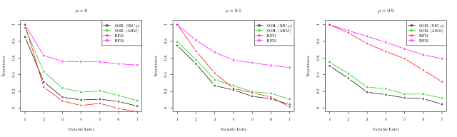
Figure 5: Simulation results for Example 5, where $n=80$, $p=6$. The true coefficients $\boldsymbol{\beta}^{*}=\left(1,\frac{1}{2},\frac{1}{3},\frac{1}{4},\frac{1}{5},\frac{1}{6},0\right){}^{\intercal}$.

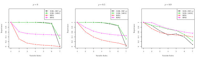
Figure 6: Simulation results for Example 6, where $n=5000$, $p=6$. The true coefficients $\boldsymbol{\beta}^{*}=\left(1,\frac{1}{2},\frac{1}{3},\frac{1}{4},\frac{1}{5},\frac{1}{6},0\right){}^{\intercal}$.

SOIL is certainly incapable of giving high importance to very weak variables in the true model. For example Figure 5 shows that in a binomial model with the decreasing coefficient vector $\boldsymbol{\beta}^{*}=\left(1,\frac{1}{2},\frac{1}{3},\frac{1}{4},\frac{1}{5},\frac{1}{6},0\right){}^{\intercal}$, the true variable $X_{6}$’s SOIL importance is only around 0.1, not much above that of the noise variable $X_{7})$. However this problem is alleviated as the sample increases: Figure 6 shows that the SOIL-ARM and SOIL-BIC-p importances of six true variables $(X_{1},\ldots,X_{6})$ become closer to one when $n$ increases from 80 to 5000. In contrast, the LMG, RFI1, and RFI2 stay basically the same as the sample size increases.

Tuning in to information.

For high dimensional data, more often than not (to say the least), sparsity is a reluctant acceptance that the info and/or computational limit only allows us a simple model for application. The optimal sparsity should depend on the sample size and noise level. Therefore, it is desirable to have an importance measure to honor this perspective. When the sample size increases or the noise decreases, we should have more information. Thus, the importance obtained from the data should change due to the enrichment of information. Therefore in most examples, when the correlation $\rho$ and $\sigma^{2}$ are low, one may hope the variable importances delineate the true model. Comparing Examples 5 and 6, which differ only in the sample size, as shown in Figure 5 and Figure 6, only SOIL-BIC-p and SOIL-ARM react to the much increased information due to sample size increase, while the other three importances are not tuned in to the information change.

Robustness to feature correlation.

SOIL importances show robustness against noise increase and higher feature correlation. For example in Figure 1, 2 and Figure S1–S5 in Supplementary Materials Part B, even when there is high feature correlation $(\rho=0.9,\sigma^{2}=0.01)$ or strong noise $(\rho=0,\sigma^{2}=25)$ in the data, the SOIL-BIC-p and SOIL-ARM can still select the true variable $X_{5}$ while the other methods consider $X_{5}$ as unimportant. But in a case of both high feature correlation and strong noise $(\rho=0.9,\sigma^{2}=25)$, none of the importance measures in comparison can quite clearly select $X_{5}$ as an important variable because the information is too limited.

Robustness against confusers.

A confuser refers to a variable that is closely related to a true variable or some linear combination of the true variables but not to the extent of serving as a valid alternative. An importance measure oriented towards sparse modeling should assign near zero importances on the confusers. The simulation results show that the SOIL importance measures are much more robust to confusers than LMG, RFI1 and RFI2. In Example 2, we generate a confuser $X_{15}=0.5X_{1}+2X_{4}+e$ with Gaussian noise $e\sim N(0,0.01)$. The results in Figure 2 show that LMG, RFI1 and RFI2 fail to assign small importance to $X_{15}$ (not in the true model) and view it more important than some true variables. In contrast, small ARM and BIC-p importances for $X_{15}$ correctly indicate that it is unimportant.

Sensitivity to higher-order terms.

The SOIL importance measures are more sensitive to inclusion of higher-order terms in the model. In Example S2 and S3 we add quadratic terms $X_{1}^{2}$, $X_{2}^{2}$, $X_{3}^{2}$, $X_{4}^{2}$, $X_{5}^{2}$, $X_{6}^{2}$ and pairwise interactions $X_{1}X_{2}$, $X_{1}X_{3}$, $X_{1}X_{4}$, $X_{2}X_{3}$, $X_{2}X_{4}$, $X_{3}X_{4}$ respectively, where the coefficients for $X_{1}X_{2}$, $X_{1}X_{3}$, $X_{1}X_{4}$ and $X_{1}^{2}$, $X_{3}^{2}$ are nonzero in the true models. Results in Figure S2 and S3 show that the ARM and BIC-p methods can select both true main-effect variables and true higher-order terms, whereas LMG, RFI1 and RFI2 fail to select some of the main-effect variables when interactions or quadratic terms are included.

Pure relativity.

An importance measure is said to be purely relative if the values individually do not have a sensible meaning on their own. One drawback of an importance measure with pure relativity is that it does not differentiate between equal importance and equal unimportance cases. All coefficients in Example 3 and 4 have the same relative size, which are $\boldsymbol{\beta}^{*}=(0,\ldots,0){}^{\intercal}$ and $\boldsymbol{\beta}^{*}=(1,\ldots,1){}^{\intercal}$ respectively. We find that LMG, RFI1 and RFI2 do not offer any clue on importance of each variable itself. Variables $(X_{1},\ldots,X_{6})$ in Example 3 have very similar LMG and RFI2 values to those in Example 4. And RFI1 behaves wildly as it assigns very much different importances to the variables in the independence case ($\rho=0$) of Example 3. The importance values are even significantly negative for some variables. In contrast, SOIL-BIC-p and SOIL-ARM nicely separate the two examples.

Order preserving.

Order preserving refers to the property that the importance reflects the “order” of the variables or not: (1) For the true variables (standardized) with not too high correlations with others, it may be natural to expect the ones with larger coefficients to have larger importances (up to one of course); (2) The true variables should have larger importances compared to the noise ones. In the case that the sample size is too small for some true variables to be detectable, the order preserving property demands that the noise variables should not receive significantly higher importance values than these subtle true variables. SOIL-BIC-p and SOIL-ARM exhibit the order preserving property in all the cases. LMG behaves poorly when there exists a confuser as in Figure 2. RFI1 and RFI2 do not preserve the order when correlation $\rho=0.9$ and/or noise $\sigma^{2}$ is large.

High-dimensionality.

SOIL-BIC-p, SOIL-ARM, RFI1 and RFI2 can work for high-dimensional data when $p>n$ as shown in Figure 1 and S5. The exclusion and inclusion properties still hold for SOIL-BIC-p and SOIL-ARM in the high dimensional case (inclusion of a weak variable requires that $\sigma^{2}$ is not too high). In contrast, LMG does not support high-dimensional data.

Non-negativity.

SOIL-BIC-p, SOIL-ARM, LMG and IMG2 always yield non-negative importance value. However, RFI1 does not satisfy this criterion.

Non-parametricness.

Among the importance measures, only the two from random forest are not limited to parametric modeling.

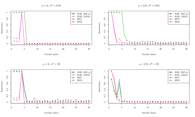
Figure 1: Simulation results for Example 1, where $n=100$, $p=200$. The true coefficients $\boldsymbol{\beta}^{*}=(4,4,4,-6\sqrt{2},\frac{3}{4},0,...,0)$.

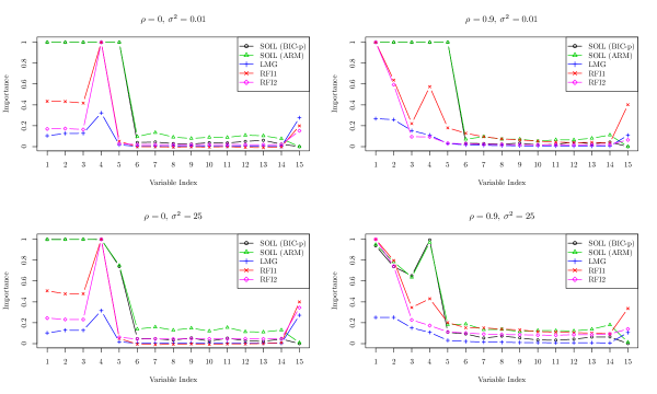
Figure 2: Simulation results for Example 2, where $n=150$, $p=14$. The true coefficients $\boldsymbol{\beta}^{*}=(4,4,4,-6\sqrt{2},\frac{3}{4},0,...,0)$. Add $X_{15}=0.5*X_{1}+2*X_{4}+e$ and corresponding $\beta_{15}^{*}=0$, where $e\sim N(0,\sigma_{e}^{2})$.

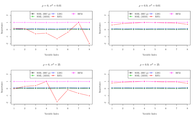
Figure 3: Simulation results for Example 3, where $n=150$, $p=8$. The true coefficients $\boldsymbol{\beta}^{*}=(0,\ldots,0)^{\intercal}$.

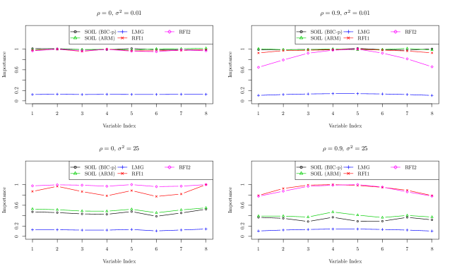
Figure 4: Simulation results for Example 4, where $n=150$, $p=8$. The true coefficients $\boldsymbol{\beta}^{*}=(1,\ldots,1)^{\intercal}$.

5.2.   Comparison with stability selection

Meinshausen & Bühlmann (2010) proposed a stability selection (SS) method to improve the Lasso variable selection. SS may be regarded as an importance measure. In Supplementary Materials Part C, we present a comparison of SS importance to our SOIL approach. Due to worse performances of SS compared with SOIL, together with the fact that the main goal of SS is not on variable importance, we do not consider SS in our main simulation.

6.   REAL DATA EXAMPLES

We apply the variable importance measures to two real datasets:

BGS data.

We first consider a dataset with small $p$ from the Berkeley Guidance Study (BGS) by Tuddenham & Snyder (1954). The dataset includes 66 registered newborn boys whose physical growth measures are followed for 18 years. Following Cook & Weisberg (2009, p.179) we consider a regression model of age 18 height on $p=6$ predictors: weights at ages two (WT2) and nine (WT9), heights at ages two (HT2) and nine (HT9), age nine leg circumference (LG9), and age 18 strength (ST18). The corresponding SOIL-ARM, SOIL-BIC-p, LMG, RFI1 and RFI2 importances for each variable are computed and summarized in Table 3. We found that HT9 is the most important variable according to all methods. But different methods produce different second-most important variables.

	WT2		HT2		WT9		HT9		LG9		ST18
SOIL-ARM	0.	16	0.	09	0.	03	1.	00	0.	62	0.	28
SOIL-BIC-p	0.	01	0.	00	0.	00	1.	00	0.	63	0.	08
LMG	0.	06	0.	13	0.	08	0.	65	0.	05	0.	02
RFI1	1.	72	2.	50	1.	79	55.	66	4.	12	1.	05
RFI2	70.	89	101.	58	100.	52	2126.	64	123.	52	127.	74

Table 3: Importances measures of the variables in BGS data. The top two most important variables according to each measure are in bold.

Then we conduct a “credibility check” for the above results of various importance measures. To do so we use a guided simulation or cross-examination (Li et al., 2000; Rolling & Yang, 2014), in which the performances of the importance measures are tested using data that are simulated from models recommended by the importance measures respectively. The basic idea of cross-examination is that one usually anticipates that a good method should have a better performance than other methods on the simulated data that are constructed from the method itself. In our context, if we compute the variable importances $S_{1}^{A},\ldots,S_{p}^{A}$ on a real dataset using measure $A$, and construct a suggested model (with top rated important variables) and simulate a new dataset from this model, then on the new dataset, the variable importances $\tilde{S}_{1}^{A},\ldots,\tilde{S}_{p}^{A}$ using measure $A$ should be more similar to $S_{1}^{A},\ldots,S_{p}^{A}$ than the variable importances $\tilde{S}_{1}^{B},\ldots,\tilde{S}_{p}^{B}$ using measure $B$. Otherwise, one can naturally question the adequacy of applying measure $A$ to the original real data.

The cross-examination procedure is as follows:

1. Choose one measure from SOIL-ARM, SOIL-BIC-p, LMG, RFI1 and RFI2 as the base measure, and select the resulting top two most important variables (e.g. HT9 and LG9 if SOIL-ARM is the base measure).

2. Fit linear regression using only the selected variables as predictors, and obtain the estimated coefficients $\boldsymbol{\widehat{\beta}}$ and standard deviation $\widehat{\sigma}$.

3. Generate the new response according to the model: ${\bf Y}_{new}=\mathbf{X}\boldsymbol{\widehat{\beta}}+\widehat{\sigma}N(0,1)$.

4. Compute the SOIL-ARM, SOIL-BIC-p, LMG, RFI1 and RFI2 importance measures using the new dataset $({\bf X},{\bf Y}_{new})$.

5. Repeat the above steps 100 times and take the average of each importance.

6. Go to Step 1 until all measures have served as the base measure.

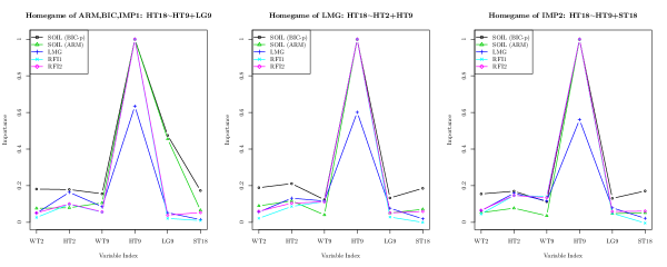
Figure 7: Results of cross-examination for BGS data.

The results are depicted in Figure 7. Overall, SOIL-ARM and SOIL-BIC-p perform reasonably better than the other importance measures. In the home-game (when the variable is selected as the base measure) of SOIL-ARM, SOIL-BIC-p and RFI1, we can see that LMG and random forest (RFI1 or RFI2) do not support the true variable LG9, while SOIL-ARM or SOIL-BIC-p clearly indicate, correctly, HT9 and LG9 as the important ones (although with less confidence on LG9). In fact, LMG, RFI1 and RFI2 all view HT2 as more important than LG9, a mistake seemingly caused by the higher correlation of HT2 (0.57) to HT18 than LG9 (0.37). In the home-game of LMG, all methods single out only HT9 as the most important (but not HT2). However, SOIL-ARM and SOIL-BIC-p assign the second largest importance to HT2, which is consistent with the aforementioned Order Preserving property. The random forest importance measures do not show this property. The home-game of RFI2 is similar to the home-game of LMG, where the Order Preserving property still holds for SOIL-ARM and SOIL-BIC-p but not for the others.

Bardet data.

For a dataset with large $p$, we consider the Bardet dataset. It collects tissue samples from the eyes of 120 twelve-week-old male rats, which are the offspring of inter-crossed F1 animals. For each tissue, the RNAs of 31,042 selected probes are measured by the normalized intensity valued. The gene intensity values are in log scale. To investigate the genes that are related to gene TRIM32, which causes the Bardet-Biedl syndrome according to Chiang et al. (2006), a screening method (Huang et al., 2008) is applied to the original probes, which gives us a dataset with 200 probes for each of 120 tissues. We use this screened dataset to carry out our importance measure analysis.

Since LMG is not feasible to handle cases with $p>20$, it is not included in our analysis below. The corresponding SOIL-ARM, SOIL-BIC-p, RFI1 and RFI2 importances for most relevant variable are summarized in Table 4. We present the top ten variables according to the different importance measures respectively. The name of each gene is too long, so for convenience we record the corresponding EST number instead. From Table 4, we can see that different importance measures have very different results.

Rank	ARM		BIC-p		RFI1		RFI2
1	25141	1.000	25141	1.000	25141	5.113	21907	0.061
2	28967	0.935	28967	1.000	21907	5.006	25141	0.059
3	28680	0.834	28680	0.999	11711	4.875	11711	0.054
4	30141	0.576	30141	0.491	11719	4.778	25105	0.041
5	21092	0.397	21092	0.278	25105	4.491	24565	0.036
6	15863	0.261	15863	0.142	9303	4.332	28680	0.035
7	17599	0.219	17599	0.121	28680	4.239	25403	0.034
8	22813	0.106	25367	0.028	25425	3.788	9303	0.033
9	25367	0.079	22813	0.016	16569	3.733	22029	0.032
10	24892	0.047	14949	0.005	22029	3.680	24087	0.030

Table 4: Top ten genes for different variable importance measures for Bardet data.

Notice that $X_{25141}$ is the most important variable according to Table 4. Random forest is unstable in the sense that each time we compute the random forest importance on the data, the top ten variables obtained tended to be quite different in terms of their rankings. For SOIL-BIC-p and SOIL-ARM, the top four genes always have the same rank and the importance values are pretty much the same in different runs. Also, a striking feature for the random forest in this data example is that the values of the importances are quite close to each other and decaying gradually, making it hard to judge which variables are really important.

We carry out a guided simulation study similar to that for the BGS data, except that LMG is not included. Based on the information in Table 4, the top 4 variables are selected for SOIL-BIC-p (SOIL-ARM), and the top 10 for RFI1 and RFI2 respectively.

In Figure 8, we only present the variable importances of the “true” genes due to space limitation. RFI1 and RFI2 are all normalized. In the home-game of SOIL-ARM and SOIL-BIC-p, both can correctly select all the true variables if the cut-off value is set at $0.4$. For random forest, however, the maximum RFI1 and RFI2 values among the unimportant ones exceed the most important ones respectively, indicating that the random forest has difficulty differentiating the really important and unimportant variables.

In the home-game of RFI1 and RFI2, none of the competitors performs very well. With the generating model being larger, with the limited information in the data (in conjunction with the complicated correlation among the genes), the importance measures simply cannot reveal all the true variables. Only the true variable $X_{25414}$ is differentiated clearly by all methods. From the SOIL perspective, it is willing to support at most 3 more variables with some confidence. Random forest gives more true variables significant importance values. A drawback is that some noise variables receive relatively large importance values, which are even higher than almost half of the true variables.

From the guided simulations, the Order Preserving property fails in all the cases for the random forest importance measures. For SOIL, in the home-game of ARM and BIC-p, it holds for both SOIL-ARM and SOIL-BIC-p; but in the home-game of RFI1 or RFI2, the property does not hold exactly, but it does hold in the sense that the maximum importance of the noise variables is still very small (and it is not meaningful to rank the variables with tiny importance values). The key point here is that while SOIL certainly can miss subtle variables in the true model when the sample size is small, it typically does not recommend an unimportant variable as important. The same cannot be said for the other importance measures.

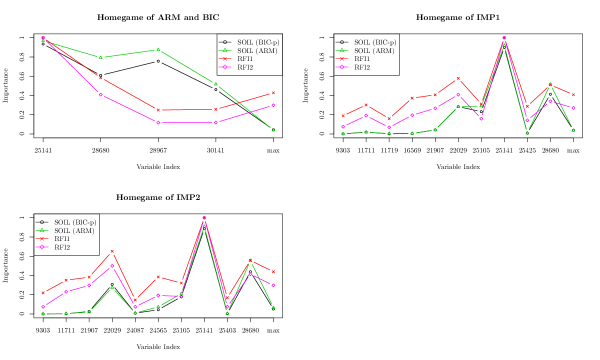
Figure 8: Simulation results for cross-examination

7.   CONCLUSION AND DISCUSSION

Variable importance is aimed to find the important variables for explanation or prediction of the response. The motivation is most natural but the task of devising an importance measure is quite tricky. Several challenges immediately arrive: 1. Importance depends on the goal of the analysis and application. Different goals may require different importance measures. 2. Should importance be based on parametric models or nonparametric models? Both seem to be valuable in our view. 3. Should the importance measure be purely relative to compare different variables or should their values have some meaning on their own?

The topic is even controversial, with attitude ranging from enthusiasm in research and/or application, to reluctant acceptance as a practical approach to deal with many predictors, to total pessimism on the topic that dismisses the possibility of general successes. The different opinions are all valid, properly reflecting the complexity and multi-facet nature of the problem.

In our opinion, there are two important facts to keep in mind. One is that people crave for importance measures, love ranking, and they put them in use. This calls for more research on the topic. The other is the currently still dominating practice of “winner-takes-all”, which is definitely a culprit of irreproducibility of many research results. For reasonably complex data, making inference and decision based on a final selected model can lead to severely biased conclusions. A reliable importance measure can provide much needed complementary information to that from a final model and substantially improve the reliability of data analysis.

We have investigated the variable importance in linear regression and classification cases. The proposed new variable importance measure (SOIL) is driven by model combination for considering more than a single model, thus giving us an understanding of all the variables, instead of only the “important” ones in view of a single model. It is seen from both the simulation results and the real data examples that the SOIL approach has several desirable features such as exclusion/inclusion, order preserving and robustness in several aspects, and performs very well compared to other variable importance measures considered.

As Grömping (2015) pointed out in her paper, there is no commonly accepted theoretical framework in the variable importance area. Not surprisingly, many critiques on variable importance measures come up. Ehrenberg (1990) pointed out that one should focus on the underneath causal mechanism instead of the relative importance. We think SOIL is satisfactory in this regard. First, given enough information, SOIL assigns variable importance close to one for these true predictors, which is consistent with revealing the causal relationship between the response and the predictors. Second, the SOIL importance of a variable goes beyond relative assessment of the variables and it gives an absolute sense on how much a variable is needed in the linear modeling with the available information. In regression settings, data analysts often use $t$ statistic or $p$-value to see if a variable is significant or not. Kruskal & Majors (1989) pointed out that this pertains to a different concept. In their view, variable importance is a population property while significance is a property of both population and sample. To us, since all models are only approximations to model the data, there is advantage to treat variable importance measures as data dependent quantities that reflect the nature of the data. SOIL intends to do just that.

Note that the two importance measures by the random forecast are not based on parametric modeling. When the GLM framework does not work for the data, our SOIL approach may not provide valuable information while random forest based ones may.

To be fair, it may be debatable if a variable that has some predictive power (one way or another) but is not needed in the best model should be given significant (reasonably strong) importance or not. Our view is that it seems rare to consider the covariates only individually and thus it is better to reflect the goal of finding the best set of covariates to explain the response in the importance measures. From this angle, while giving out relevant variables is certainly useful, it may not be the most essential from a modeling perspective.

Through our simulation work, we have shown that the other methods often give clearly higher importance to variables that are not in the true model and/or give lower values for some variables in the true model when the covariates are correlated, error variance is large, or there are interaction terms. In real applications, these situations occur rather commonly. Thus the results seem to suggest that when sparse modeling is the goal, those importance measures may not directly provide objective variable assessment information.

APPENDIX

Proof of Theorem 1.

Proof.

Denote by $\mathcal{A}^{*}\backslash\mathcal{A}^{k}$ the set of variables contained in $\mathcal{A}^{*}$ but not in $\mathcal{A}^{k}$. Since

$$\dfrac{\sum_{k=1}^{K}w_{k}|\mathcal{A}^{*}\backslash\mathcal{A}^{k}|}{r^{*}} = \dfrac{\sum_{k=1}^{K}w_{k}\sum_{j\in\mathcal{A}^{*}}I(j\notin\mathcal{A}^{k})}{r^{*}}$$

$$= \dfrac{\sum_{j\in\mathcal{A}^{*}}\sum_{k=1}^{K}w_{k}I(j\notin\mathcal{A}^{k})}{r^{*}}$$

$$= \dfrac{\sum_{j\in\mathcal{A}^{*}}\sum_{k=1}^{K}w_{k}(1-I(j\in\mathcal{A}^{k}))}{r^{*}}$$

$$= \dfrac{\sum_{j\in\mathcal{A}^{*}}(1-S_{j})}{r^{*}}.$$

and by the definition of weak consistency,

$$0\leq\dfrac{\sum_{k=1}^{K}w_{k}|\mathcal{A}^{*}\backslash\mathcal{A}^{k}|}{r^{*}}\leq\dfrac{\sum_{k=1}^{K}w_{k}|\mathcal{A}^{k}\nabla\mathcal{A}^{*}|}{r^{*}}{\displaystyle\ \overset{p}{\to}\ }0.$$

Hence,

$$\dfrac{\sum_{j\in\mathcal{A}^{*}}(1-S_{j})}{r^{*}} {\displaystyle\overset{p}{\to}} 0.$$

On the other hand,

$$\dfrac{\sum_{j\notin\mathcal{A}^{*}}S_{j}}{r^{*}} = \dfrac{\sum_{j\notin\mathcal{A}^{*}}\sum_{k=1}^{K}w_{k}I(j\in\mathcal{A}^{k})}{r^{*}}$$

$$= \dfrac{\sum_{k=1}^{K}w_{k}\sum_{j\notin\mathcal{A}^{*}}I(j\in\mathcal{A}^{k})}{r^{*}}$$

$$= \dfrac{\sum_{k=1}^{K}w_{k}|\mathcal{A}^{k}\backslash\mathcal{A}^{*}|}{r^{*}}$$

$$\leq \dfrac{\sum_{k=1}^{K}w_{k}|\mathcal{A}^{k}\nabla\mathcal{A}^{*}|}{r^{*}}\overset{p}{\to}0.$$

∎

Proof of Theorem 2.

Assume $\dfrac{|\overline{\mathcal{A}}_{c}|}{r^{*}}$ does not converge to $0$ in probability as $n$ tends to infinity ($r^{*}$ may or may not depend on $n$), then we have a subsequence , which for convenience we still denote by $\dfrac{|\overline{\mathcal{A}}_{c}|}{r^{*}}$, that is greater than a non-zero positive constant $\epsilon_{0}$, i.e. $\dfrac{|\overline{\mathcal{A}}_{c}|}{r^{*}}\geq\epsilon_{0}$ in probability. Thus,

$$\dfrac{\sum_{j\in\mathcal{A}^{*}}(1-S_{j})}{r^{*}} = \dfrac{\sum_{j\in\mathcal{A}^{*},S_{j}\leq c}(1-S_{j})}{r^{*}}+\dfrac{\sum_{j\in\mathcal{A}^{*},S_{j}>c}(1-S_{j})}{r^{*}}$$

$$\geq \dfrac{\sum_{j\in\mathcal{A}^{*},S_{j}\leq c}(1-S_{j})}{r^{*}}$$

$$\geq \dfrac{\sum_{j\in\mathcal{A}^{*},S_{j}\leq c}(1-c)}{r^{*}}$$

$$= (1-c)\dfrac{\sum_{j\in\mathcal{A}^{*}}I(S_{j}\leq c)}{r^{*}}$$

$$= (1-c)\dfrac{|\overline{\mathcal{A}}_{c}|}{r^{*}}$$

$$\geq (1-c)\epsilon_{0},$$

which contradicts with Theorem 2. Hence, we have $\dfrac{|\overline{\mathcal{A}}_{c}|}{r^{*}}{\displaystyle\ \overset{p}{\to}\ }0.$ Similarly, we can prove $\dfrac{|\underline{\mathcal{A}}_{c}|}{r^{*}}{\displaystyle\ \overset{p}{\to}\ }0$. ∎

SUPPLEMENTARY MATERIALS

R-package for SOIL:

R-package SOIL containing code to compute the SOIL importance measure described in the article. (GNU zipped tar file)

Real data sets:

Data sets BGS and Bardet used in the illustration of SOIL in Section 6. (.rda file)

Text document:

Supplementary materials for “Sparsity Oriented Importance Learning for High-dimensional Linear Regression” by Chenglong Ye, Yi Yang and Yuhong Yang. (.pdf file)

Supplemental Materials for “Sparsity Oriented Importance Learning for High-dimensional Linear Regression”

Part A: Weighting using generalized fiducial inference.

Based on Fisher’s controversial fiducial idea, Lai et al. (2015) proposed the generalized fiducial inference applied to “large $p$ small $n$” problem. Their paper concerns the generalized fiducial inference for the linear regression case. For each candidate model $\mathcal{A}^{k}$, the fiducial probability for the model is

$$p(\mathcal{A}^{k})\propto R(\mathcal{A}^{k})\equiv\Gamma(\frac{n-\left|\mathcal{A}^{k}\right|}{2})(\pi RSS_{\mathcal{A}^{k}})^{-\frac{n-\left|\mathcal{A}^{k}\right|-1}{2}}n^{-\frac{\left|\mathcal{A}^{k}\right|+1}{2}}\left(\begin{array}[]{c}p\\ \left|\mathcal{A}^{k}\right|\end{array}\right)^{-\gamma},$$

where $RSS_{\mathcal{A}^{k}}$ is the residual sum of squares of $\mathcal{A}^{k}$. For a practical reason, the authors approximate the above fiducial probability by

$$r(\mathcal{A}^{k})\approx R(\mathcal{A}^{k})/\sum_{l=1}^{K}R(\mathcal{A}^{l}).$$

We can use $r(\mathcal{A}^{k})$ as the weight $w_{k}$ for each candidate model. It is shown in their paper that the true model will have the highest fiducial probability among all the candidate models.

Part B: Additional simulation results.

In this part, we provide the results of Example S1-S5, whose settings are described in Table 1 of the main body of the article. These results support our conclusions as discussed in Section 5.1.

Figure S1: Simulation results for Example S1, where $n=150$, $p=20$. The true coefficients $\boldsymbol{\beta}^{*}=(4,4,4,-6\sqrt{2},\frac{3}{4},0,...,0)$.

Figure S2: Simulation results for Example S2, where $n=150$, $p=6$. The true coefficients $\boldsymbol{\beta}^{*}=(4,4,-6\sqrt{2},\frac{3}{4},0,0)^{\intercal}$. Add $(X_{1}^{2},X_{2}^{2},X_{3}^{2},X_{4}^{2},X_{5}^{2},X_{6}^{2})$ and corresponding coefficients $(\beta_{7}^{*},\beta_{8}^{*},\ldots,\beta_{12}^{*})^{\intercal}=(4,0,1,0,0,0)^{\intercal}$.

Figure S3: Simulation results for Example S3, where $n=150$, $p=6$. The true coefficient $\boldsymbol{\beta}^{*}=(4,4,-6\sqrt{2},\frac{3}{4},0,0)^{\intercal}$. Add $(X_{1}X_{2},X_{1}X_{3},X_{1}X_{4},X_{2}X_{3},X_{2}X_{4},X_{3}X_{4})$ and corresponding coefficients $(\beta_{7}^{*},\beta_{8}^{*},\ldots,\beta_{12}^{*})^{\intercal}=(4,2,2,0,0,0)^{\intercal}$.

Figure S4: Simulation results for Example S4, where $n=150$, $p=20$. The true coefficients $\boldsymbol{\beta}^{*}=(4,4,4,-6\sqrt{2},\frac{3}{4},0,...,0)$.

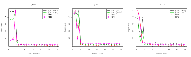
Figure S5: Simulation results for Example S5, where $n=100$, $p=200$. The true coefficients $\boldsymbol{\beta}^{*}=(4,4,4,-6\sqrt{2},\frac{3}{4},0,...,0)$.

Part C: Comparison with stability selection.

In this subsection, we present a comparison of SS (Meinshausen & Bühlmann 2010) importance to our SOIL importance.

The simulation data $\{y_{i},\mathbf{x}_{i}\}_{i=1}^{n}$ is generated from the linear model $y_{i}=\mathbf{x}_{i}^{\intercal}\boldsymbol{\beta}^{*}+\epsilon_{i}$, $\epsilon\sim N(0,\sigma^{2})$. We generate $\mathbf{x}_{i}$ from multivariate normal distribution $N_{p}(0,\Sigma)$. For each element $\Sigma_{ij}$ of $\Sigma$, $\Sigma_{ij}=\rho^{\left|i-j\right|}$, i.e. the correlation of $X_{i}$ and $X_{j}$ is $\rho^{\left|i-j\right|}$. We consider two cases, the settings of which are listed in Table S1.

Example	$n$	$p$	$\rho$	$\sigma^{2}$	Coefficients
1	100	20	0	0.01	$\boldsymbol{\beta}^{*}=(4,4,4,-6\sqrt{2},\frac{3}{4},0,...,0)^{\intercal}$
2	100	20	0.7	0.1	$\boldsymbol{\beta}^{*}=(4,0,4,-6\sqrt{2},\frac{3}{4},0,...,0)^{\intercal}$

Table S1: Simulation settings for SS

It can be seen from Tables S2 and S3 that SS does not give enough importance to the true variable $X_{5}$ in Example 1 while it more strongly supports the noise variable $X_{2}$ than the true variable $X_{5}$ in Example 2, which leads to unavoidable incorrect variable selection regardless of the cutoff to be used to decide if a variable is in or out based on its importance. In contrast, SOIL-ARM and SOIL-BIC-p pick all the important variables and leave noise variables out. From these results, together with the fact that the main goal of SS is not on variable importance, we have not considered stability selection in the main simulations in this work.

Method/Variable	$X_{1}$	$X_{2}$	$X_{3}$	$X_{4}$	$X_{5}$	max of rest
SOIL-ARM	1.00	1.00	1.00	1.00	1.00	0.12
SOIL-BIC-p	1.00	1.00	1.00	1.00	1.00	0.07
Stability Selection	0.99	0.99	0.99	1.00	0.02	0.002

Table S2: Variable importance for Example 1.

Method/Variable	$X_{1}$	$X_{2}$	$X_{3}$	$X_{4}$	$X_{5}$	max of rest
SOIL-ARM	1.00	0.15	1.00	1.00	1.00	0.14
SOIL-BIC-p	1.00	0.06	1.00	1.00	1.00	0.05
Stability Selection	1.00	0.44	0.94	1.00	0.26	0.05

Table S3: Variable importance for Example 2.

References

- (1)
- Akaike (1973) Akaike, H. (1973), Information theory and an extension of the maximum likelihood principle, in ‘Second International Symposium on Information Theory (Tsahkadsor, 1971)’, Akadémiai Kiadó, Budapest, pp. 267–281.
- Archer & Kimes (2008) Archer, K. J. & Kimes, R. V. (2008), ‘Empirical characterization of random forest variable importance measures’, Computational Statistics & Data Analysis 52(4), 2249–2260.
- Braun & Oswald (2011) Braun, M. T. & Oswald, F. L. (2011), ‘Exploratory regression analysis: A tool for selecting models and determining predictor importance’, Behavior Research Methods 43(2), 331–339.
- Breiman (2001) Breiman, L. (2001), ‘Random forests’, Machine Learning 45(1), 5–32.
- Buckland et al. (1997) Buckland, S. T., Burnham, K. P. & Augustin, N. H. (1997), ‘Model selection: an integral part of inference’, Biometrics 53(2), 603–618.
- Budescu (1993) Budescu, D. V. (1993), ‘Dominance analysis: A new approach to the problem of relative importance of predictors in multiple regression’, Psychological Bulletin 114(3), 542.
- Chen et al. (2007) Chen, L., Giannakouros, P. & Yang, Y. (2007), ‘Model combining in factorial data analysis’, Journal of Statistical Planning and Inference 137(9), 2920–2934.
- Cheng et al. (2015) Cheng, T.-C. F., Ing, C.-K. & Yu, S.-H. (2015), ‘Toward optimal model averaging in regression models with time series errors’, Journal of Econometrics 189(2), 321–334.
- Cheng & Hansen (2015) Cheng, X. & Hansen, B. E. (2015), ‘Forecasting with factor-augmented regression: A frequentist model averaging approach’, Journal of Econometrics 186(2), 280–293.
- Chevan & Sutherland (1991) Chevan, A. & Sutherland, M. (1991), ‘Hierarchical partitioning’, The American Statistician 45(2), 90–96.
- Chiang et al. (2006) Chiang, A. P., Beck, J. S., Yen, H.-J., Tayeh, M. K., Scheetz, T. E., Swiderski, R. E., Nishimura, D. Y., Braun, T. A., Kim, K.-Y. A., Huang, J. et al. (2006), ‘Homozygosity mapping with snp arrays identifies TRIM32, an E3 ubiquitin ligase, as a Bardet–Biedl syndrome gene (BBS11)’, Proceedings of the National Academy of Sciences 103(16), 6287–6292.
- Cook & Weisberg (2009) Cook, R. D. & Weisberg, S. (2009), Applied regression including computing and graphics, Vol. 488, John Wiley & Sons.
- Ehrenberg (1990) Ehrenberg, A. S. C. (1990), ‘The unimportance of relative importance’, American Statistician 44(3), 260–260.
- Fan & Li (2001) Fan, J. & Li, R. (2001), ‘Variable selection via nonconcave penalized likelihood and its oracle properties’, Journal of the American statistical Association 96(456), 1348–1360.
- Feldman (2005) Feldman, B. E. (2005), ‘Relative importance and value’, Available at SSRN 2255827 .
- Feldman et al. (1999) Feldman, B. et al. (1999), ‘The proportional value of a cooperative game’, Manuscript. Chicago: Scudder Kemper Investments .
- Ferrari & Yang (2015) Ferrari, D. & Yang, Y. (2015), ‘Confidence sets for model selection by F-testing’, Statistica Sinica 25, 1637–1658.
- Grömping (2015) Grömping, U. (2015), ‘Variable importance in regression models’, Wiley Interdisciplinary Reviews: Computational Statistics 7(2), 137–152.
- Grömping et al. (2006) Grömping, U. et al. (2006), ‘Relative importance for linear regression in R: the package relaimpo’, Journal of Statistical Software 17(1), 1–27.
- Hansen (2007) Hansen, B. E. (2007), ‘Least squares model averaging’, Econometrica 75(4), 1175–1189.
- Hapfelmeier et al. (2014) Hapfelmeier, A., Hothorn, T., Ulm, K. & Strobl, C. (2014), ‘A new variable importance measure for random forests with missing data’, Statistics and Computing 24(1), 21–34.
- Hjort & Claeskens (2003) Hjort, N. L. & Claeskens, G. (2003), ‘Frequentist model average estimators’, Journal of the American Statistical Association 98(464), 879–899.
- Hoeting et al. (1999) Hoeting, J. A., Madigan, D., Raftery, A. E. & Volinsky, C. T. (1999), ‘Bayesian model averaging: a tutorial’, Statistical Science 14(4), 382–401.
- Hoffman (1960) Hoffman, P. J. (1960), ‘The paramorphic representation of clinical judgment’, Psychological Bulletin 57(2), 116.
- Huang et al. (2008) Huang, J., Ma, S. & Zhang, C.-H. (2008), ‘Adaptive Lasso for sparse high-dimensional regression models’, Statistica Sinica 18, 1603–1618.
- Ioannidis & Khoury (2011) Ioannidis, J. P. & Khoury, M. J. (2011), ‘Improving validation practices in “omics” research’, Science 334(6060), 1230–1232.
- Ishwaran (2007) Ishwaran, H. (2007), ‘Variable importance in binary regression trees and forests’, Electronic Journal of Statistics 1, 519–537.
- Kruskal & Majors (1989) Kruskal, W. & Majors, R. (1989), ‘Concepts of relative importance in recent scientific literature’, The American Statistician 43(1), 2–6.
- Lai et al. (2015) Lai, R. C., Hannig, J. & Lee, T. C. (2015), ‘Generalized fiducial inference for ultrahigh-dimensional regression’, Journal of the American Statistical Association 110(510), 760–772.
- Leung & Barron (2006) Leung, G. & Barron, A. R. (2006), ‘Information theory and mixing least-squares regressions’, IEEE Transactions on Information Theory 52(8), 3396–3410.
- Li et al. (2000) Li, K.-C., Lue, H.-H. & Chen, C.-H. (2000), ‘Interactive tree-structured regression via principal Hessian directions’, Journal of the American Statistical Association 95(450), 547–560.
- Liang et al. (2012) Liang, H., Zou, G., Wan, A. T. & Zhang, X. (2012), ‘Optimal weight choice for frequentist model average estimators’, Journal of the American Statistical Association .
-
Liaw & Wiener (2002)
Liaw, A. & Wiener, M. (2002),
‘Classification and regression by randomForest’, R News 2(3), 18–22.
http://CRAN.R-project.org/doc/Rnews/ - Lindeman et al. (1980) Lindeman, R. H., Merenda, P. F. & Gold, R. Z. (1980), Introduction to bivariate and multivariate analysis., number 519.535 L743, Scott, Foresman.
- Louppe et al. (2013) Louppe, G., Wehenkel, L., Sutera, A. & Geurts, P. (2013), Understanding variable importances in forests of randomized trees, in ‘Advances in Neural Information Processing Systems’, pp. 431–439.
- McNutt (2014) McNutt, M. (2014), ‘Raising the bar’, Science 345(6192), 9–9.