Server assisted distributed cooperative localization over unreliable communication links

Abstract

This paper considers the problem of cooperative localization (CL) using inter-robot measurements for a group of networked robots with limited on-board resources. We propose a novel recursive algorithm in which each robot localizes itself in a global coordinate frame by local dead reckoning, and opportunistically corrects its pose estimate whenever it receives a relative measurement update message from a server. The computation and storage cost per robot in terms of the size of the team is of order $O(1)$, and the robots are only required to transmit information when they are involved in a relative measurement. The server also only needs to compute and transmit update messages when it receives an inter-robot measurement. We show that under perfect communication, our algorithm is an alternative but exact implementation of a joint CL for the entire team via Extended Kalman Filter (EKF). The perfect communication however is not a hard requirement. In fact, we show that our algorithm is intrinsically robust with respect to communication failures, with formal guarantees that the updated estimates of the robots receiving the update message are of minimum variance in a first-order approximate sense at that given timestep. We demonstrate the performance of the algorithm in simulation and experiments.

Keywords: Cooperative localization; limited onboard resources; message dropouts.

I Introduction

We consider the design of a decentralized cooperative localization (CL) algorithm for a group of communicating mobile robots. Using CL, mobile robots in a team improve their positioning accuracy by jointly processing inter-robot relative measurement feedbacks. Unlike classical beacon-based localization algorithms [1] or fixed feature-based Simultaneous Localization and Mapping algorithms [2], CL does not rely on external features of the environment. As such, this approach is an appropriate localization strategy in applications that take place in a priori uncharted environments with no or intermittent GPS access.

Via CL strong correlations among the local state estimates of the robotic team members are created. Similar to any state estimation process, accounting for these cross-correlations is crucial for the consistency of CL algorithms. Since correlations create nonlinear couplings in the state estimate equations of the robots, to produce consistent results, initial implementations of CL were fully centralized. These schemes gathered and processed information at each time-step from the entire team at a single device, either by means of a leader robot or a fusion center (FC), and broadcast back the estimated location results to each robot [3, 4]. Multi-centralized CL, wherein each robot keeps a copy of the state estimate equation of the entire team and broadcasts its own information to the entire team so that every robot can reproduce the centralized pose estimate is also proposed in the literature [5]. Besides a high-processing cost for each robot, this scheme requires an all-to-all robot communication at the time of each information exchange. Developing consistent CL algorithms that account for the intrinsic cross-correlations of state estimates with reasonable communication, computation and storage costs has been an active research area for the past decade. This problem becomes more challenging if in-network communications fail due to external events such as obstacle blocking or limited communication ranges.

For applications that maintaining multi-agent connectivity is challenging, [6, 7, 8, 9, 10, 11] propose a set of algorithms in which communication is only required at the relative measurement times between the two robots involved in the measurement. As such, these schemes can update only the state estimate of one or both of these robots. To eliminate the tight connectivity requirement, instead of maintaining the exact prior robot-to-robot correlations, in [6] each robot maintains a bank of EKFs together with an accurate book-keeping of what robot estimates were used in the past to update these local filters. Computational complexity, large memory demand, and the growing size of information needed at each update time are the main drawbacks. In [7, 8, 9, 10], also the prior robot-to-robot correlations are not maintained, but are accounted for in an implicit manner using Covariance Intersection fusion (CIF) method. Because CIF uses conservative bounds to account for missing cross-covariance information, these methods often deliver highly conservative estimates. To improve estimation accuracy, [11] proposes an algorithm in which each robot, by tolerating an $O(N)$ processing and storage cost, maintains an approximate track of its prior cross-covariances with others. In another approach to relax connectivity, [12] proposes a leader-assistive CL scheme for underwater vehicles. This algorithm is a decentralized extended information filter that uses ranges and state information from a single reference source (the server) with higher navigation accuracy to improve localization accuracy of underwater vehicle(s) (the client(s)). In this scheme the server interacts with each client separately and there is no cooperation between the clients.

Despite their relaxed connectivity requirement, the algorithms of [6, 7, 8, 9, 10, 11, 12] are conservative also by nature because they do not enable other agents in the network to fully benefit from measurement updates. Recall that correlation terms are means of expanding the benefit of robot-to-robot measurement updates to the entire team (see [13] for further details). Therefore, tightly-coupled decentralized CL algorithms that maintain the correlations among the team members result in better localization accuracy. One such algorithm obtained from distributing computations of a joint EKF CL algorithm is proposed in [14], where the propagation stage is fully decentralized by splitting each cross-covariance term between the corresponding two robots. However, at update times, the separated parts should be combined, requiring either an all-to-all robot communications or bidirectional all-to-a fusion-center communications. Another decentralized CL algorithm based on decoupling the propagation stage of a joint EKF CL using an alternative but equivalent formulation of EKF CL is proposed in [13]. Unlike [14], in [13] each robot can locally reproduce the updated pose estimate and covariance of the joint EKF at the update stage, after receiving an update message only from the robot that has made the relative measurement. In both of these algorithms, for a team of $N$ robots, each robot incurs an $O(N^{2})$ processing and storage cost as they need to evolve a variable of size of the entire covariance matrix of the robotic team. Subsequently, [15] presents a maximum-a-posteriori (MAP) decentralized CL algorithm in which all the robots in the team calculate parts of the centralized CL. All the algorithms above assume that communication messages are delivered perfectly at all times. A decentralized CL approach equivalent to a centralized CL, when possible, which handles both limited communication ranges and time-varying communication graphs is proposed in [16]. This technique uses an information transfer scheme wherein each robot broadcasts all its locally available information (the past and present measurements, as well as past measurements previously received from other robots) to every robot within its communication radius at each time-step. The main drawback of this algorithm is its high communication and storage cost.

In this paper, we design a novel tightly-coupled distributed CL algorithm in which each robot localizes itself in a global coordinate frame by local dead reckoning, and opportunistically corrects its pose estimate whenever it receives a relative measurement update message from a server. The update message is broadcast any time server receives an inter-robot relative measurement and local estimates from a pair of robots in the team that were engaged in a relative measurement. In our setup, the server can be a team member with greater processing and storage capabilities. Under a perfect communication scenario, we show that our algorithm is an exact distributed implementation of a joint CL via EKF formulation. To obtain our algorithm, we use an alternative representation of EKF formulation of CL called Split-EKF for CL. Split-EKF for CL was proposed in [17] without the formal guarantee of equivalency. In this paper, we establish this guarantee via a mathematical induction proof. Our next contribution is to show that our proposed algorithm is robust to occasional message dropouts in the network. Specifically, we show that the updated estimates of robots receiving the update message are minimum variance. In our algorithm, since every robot only propagates and updates its own pose estimates, the storage and processing cost per robot is $O(1)$. Robots only need to communicate with the server if they are involved in an inter-robot measurement. Since occasional message drop-outs are allowed in our algorithm, the connectivity requirement is flexible. Moreover, we make no assumptions about the type of robots or relative measurements. Therefore, our algorithm can be employed for teams of heterogenous robots.

II Preliminaries

In this section, we describe our robotic team model and review the joint CL via EKF as well as its alternative representation Split-EKF. In the proceeding sections, we use Split-EKF to devised our proposed server assisted CL algorithm.

We consider a team of $N$ robots in which every robot has a detectable unique identifier and corresponding unique integer label belonging to the set $\mathcal{V}=\{1,\dots,N\}$. Using a set of proprioceptive sensors, robot $i\in\mathcal{V}$ measures its self-motion and uses it to dead reckon, i.e., propagate its equations of motion $\boldsymbol{\mathbf{x}}^{i}(k+1)=\boldsymbol{\mathbf{f}}^{i}(\boldsymbol{\mathbf{x}}^{i}(k),\boldsymbol{\mathbf{u}}_{m}^{i}(k))$, $k\in{\mathbb{Z}}_{\geq 0}$, where $\boldsymbol{\mathbf{x}}^{i}\in{\mathbb{R}}^{n^{i}}$ is the pose vector and $\boldsymbol{\mathbf{u}}_{m}^{i}=\boldsymbol{\mathbf{u}}^{i}+\boldsymbol{\mathbf{\eta}}^{i}\in{\mathbb{R}}^{m^{i}}$ is the measured self-motion variable (for example velocities) with $\boldsymbol{\mathbf{u}}^{i}$ being the actual value and $\boldsymbol{\mathbf{\eta}}^{i}$ the contaminating noise. The robotic team can be heterogeneous. Every robot also carries exteroceptive sensors to detect, uniquely, the other robots in the team and take relative measurements from them, e.g., range or bearing or both. We let ($i\xrightarrow{k}j$) indicate that robot $i$ has taken relative measurement from robot $j$ at time $k$. The relative measurement is modeled by

$$\boldsymbol{\mathbf{z}}_{i,j}(k) =\boldsymbol{\mathbf{h}}_{i,j}(\boldsymbol{\mathbf{x}}^{i}(k),\boldsymbol{\mathbf{x}}^{j}(k))+\boldsymbol{\mathbf{\nu}}^{i}(k),~{}~{}\boldsymbol{\mathbf{z}}_{i,j}\in^{n_{z}^{i}},$$ (1)

where $\boldsymbol{\mathbf{h}}_{i,j}(\boldsymbol{\mathbf{x}}^{i},\boldsymbol{\mathbf{x}}^{j})$ is the measurement model and $\boldsymbol{\mathbf{\nu}}^{i}$ is measurement noise. The noises $\boldsymbol{\mathbf{\eta}}^{i}$ and $\boldsymbol{\mathbf{\nu}}^{i}$, $i\in\mathcal{V}$, are independent zero-mean white Gaussian processes with known positive definite variances $\boldsymbol{\mathbf{Q}}^{i}(k)=\text{E}[{\boldsymbol{\mathbf{\eta}}^{i}}(k)\boldsymbol{\mathbf{\eta}}^{i}(k)^{\top}]$ and $\boldsymbol{\mathbf{R}}^{i}(k)\!=\!\text{E}[{\boldsymbol{\mathbf{\nu}}^{i}}(k)\boldsymbol{\mathbf{\nu}}^{i}(k)^{\top}]$. All noises are assumed to be mutually uncorrelated. In the following, we use $\mathbb{S}^{n}_{>0}$ as set of real positive definite $n\times n$ matrices.

Joint CL via EKF is obtained from applying EKF over the joint system motion model  $\boldsymbol{\mathbf{x}}(k\!+\!1)\!=\!(\boldsymbol{\mathbf{f}}^{1}(\boldsymbol{\mathbf{x}}^{1},\boldsymbol{\mathbf{u}}^{1}),\cdots,\boldsymbol{\mathbf{f}}^{N}(\boldsymbol{\mathbf{x}}^{N},$ $\boldsymbol{\mathbf{u}}^{N}))+\operatorname{Diag}(\boldsymbol{\mathbf{g}}^{1}(\boldsymbol{\mathbf{x}}^{1}),\cdots,\boldsymbol{\mathbf{g}}^{N}(\boldsymbol{\mathbf{x}}^{N}))\boldsymbol{\mathbf{\eta}}(k),$ and the relative measurement model (1) [14]. Starting at $\hat{\boldsymbol{\mathbf{x}}}^{i\mbox{+}}\!(0)\!\in\!^{n^{i}}$, $\boldsymbol{\mathbf{P}}^{i\mbox{+}}\!(0)\!\in\!\mathbb{S}^{n^{i}}_{>0}$, $\boldsymbol{\mathbf{P}}_{i,j}^{\mbox{+}}(0)\!=\!\boldsymbol{\mathbf{0}}_{n^{i}\times n^{j}}$, $i\in\mathcal{V}$ and $j\!\in\!\mathcal{V}\backslash\{i\}$, the propagation and update equations of the EKF CL are

$$\!\!\!\hat{\boldsymbol{\mathbf{x}}}^{i\mbox{-}}(k\!+\!1)\!=\boldsymbol{\mathbf{f}}^{i}(\hat{\boldsymbol{\mathbf{x}}}^{i\mbox{+}}(k),\boldsymbol{\mathbf{u}}^{i}(k)),$$ (2a)

$$\!\!\!\boldsymbol{\mathbf{P}}^{i\mbox{-}}(k\!+\!1)\!=\boldsymbol{\mathbf{F}}^{i}(k)\boldsymbol{\mathbf{P}}^{i\mbox{+}}(k)\boldsymbol{\mathbf{F}}^{i}(k)\!^{\top}\!\!\!+\!\boldsymbol{\mathbf{G}}^{i}(k)\boldsymbol{\mathbf{Q}}^{i}(k)\boldsymbol{\mathbf{G}}^{i}(k)\!^{\top}\!\!\!,$$ (2b)

$$\!\!\!\boldsymbol{\mathbf{P}}_{i,j}^{\mbox{-}}(k\!+\!1)\!=\boldsymbol{\mathbf{F}}^{i}(k)\boldsymbol{\mathbf{P}}_{i,j}^{\mbox{+}}(k){\boldsymbol{\mathbf{F}}^{j}(k)}\!^{\top}\!\!,$$ (2c)

$$\!\!\!\hat{\boldsymbol{\mathbf{x}}}^{i\mbox{+}}(k\!+\!1)\!=\hat{\boldsymbol{\mathbf{x}}}^{i\mbox{-}}(k\!+\!1)+\boldsymbol{\mathbf{K}}_{i}(k\!+\!1)\boldsymbol{\mathbf{r}}^{a}(k\!+\!1),$$ (2d)

$$\!\!\!\boldsymbol{\mathbf{P}}^{\!i\mbox{+}}(k\!+\!1)\!=\boldsymbol{\mathbf{P}}^{\!i\mbox{-}}\!(k\!+\!1)\!-\!\boldsymbol{\mathbf{K}}_{i}(k\!+\!1)\boldsymbol{\mathbf{S}}_{a,b}(k\!+\!1)\boldsymbol{\mathbf{K}}_{i}(k\!+\!1)\!\!^{\top}\!\!\!,$$ (2e)

$$\!\!\!\boldsymbol{\mathbf{P}}_{\!i,j}^{\mbox{+}}(k\!+\!1)\!=\boldsymbol{\mathbf{P}}_{\!i,j}^{\mbox{-}}(k\!+\!1)\!-\!\boldsymbol{\mathbf{K}}_{\!i}(k\!+\!1)\boldsymbol{\mathbf{S}}_{a,b}(k\!+\!1)\boldsymbol{\mathbf{K}}_{\!j}(k\!+\!1)\!^{\top}\!\!\!,$$ (2f)

$$\!\!\!\boldsymbol{\mathbf{K}}_{i}(k\!+\!1)=$$ (2g)

$$\begin{cases}\boldsymbol{\mathbf{0}},\qquad\qquad\qquad\qquad~{}\text{no relative measurement at~{}}k\!+\!1,\\ (\boldsymbol{\mathbf{P}}_{i,b}^{\mbox{-}}(k\!+\!1)\tilde{\boldsymbol{\mathbf{H}}}_{b}^{\top}\!+\!\boldsymbol{\mathbf{P}}_{i,a}^{\mbox{-}}(k\!+\!1)\tilde{\boldsymbol{\mathbf{H}}}_{a}^{\top}){\boldsymbol{\mathbf{S}}_{a,b}}^{-1}\!,\qquad~{}a\xrightarrow{k+1}b.\end{cases}$$

for $k\in{\mathbb{Z}}_{\geq 0}$, with $\boldsymbol{\mathbf{F}}^{i}=\partial\boldsymbol{\mathbf{f}}(\hat{\boldsymbol{\mathbf{x}}}^{i\mbox{+}},\boldsymbol{\mathbf{u}}_{m}^{i})/\partial\boldsymbol{\mathbf{x}}^{i}|_{\hat{\boldsymbol{\mathbf{x}}}^{i},\boldsymbol{\mathbf{u}}^{i}_{m}=\boldsymbol{\mathbf{0}}}$ and $\boldsymbol{\mathbf{G}}^{i}=\partial\boldsymbol{\mathbf{f}}(\hat{\boldsymbol{\mathbf{x}}}^{i\mbox{+}},\boldsymbol{\mathbf{u}}_{m}^{i})/\partial\boldsymbol{\mathbf{\eta}}^{i}|_{\hat{\boldsymbol{\mathbf{x}}}^{i},\boldsymbol{\mathbf{u}}^{i}_{m}=\boldsymbol{\mathbf{0}}}$. Moreover, when a robot $a$ takes a relative measurement from robot $b$ at some given time $k+1$, the measurement residual and its covariance are, respectively,

$$\!\!\!\boldsymbol{\mathbf{r}}^{a}(k\!+\!1)\! =\boldsymbol{\mathbf{z}}_{a,b}(k\!+\!1)\!-\!\boldsymbol{\mathbf{h}}_{a,b}(\hat{\boldsymbol{\mathbf{x}}}^{a\mbox{-}}(k\!+\!1),\hat{\boldsymbol{\mathbf{x}}}^{b\mbox{-}}(k\!+\!1)),$$ (3a)

$$\!\!\boldsymbol{\mathbf{S}}_{a,b}(k\!+\!1)\!\! =\!\boldsymbol{\mathbf{R}}^{a}(k\!+\!1)+\tilde{\boldsymbol{\mathbf{H}}}_{a}(k\!+\!1)\boldsymbol{\mathbf{P}}^{a\mbox{-}}(k\!+\!1)\tilde{\boldsymbol{\mathbf{H}}}_{a}(k\!+\!1)\!^{\top}$$

$$~{}~{}+\tilde{\boldsymbol{\mathbf{H}}}_{b}(k+1)\boldsymbol{\mathbf{P}}^{b\mbox{-}}(k+1)\tilde{\boldsymbol{\mathbf{H}}}_{b}(k+1)^{\top}$$ (3b)

$$~{}~{}+\tilde{\boldsymbol{\mathbf{H}}}_{b}(k+1)\boldsymbol{\mathbf{P}}_{ba}^{\mbox{-}}(k+1){\tilde{\boldsymbol{\mathbf{H}}}_{a}}(k+1)^{\top}$$

$$~{}~{}+\tilde{\boldsymbol{\mathbf{H}}}_{a}(k+1)\boldsymbol{\mathbf{P}}_{a,b}^{\mbox{-}}(k+1)\tilde{\boldsymbol{\mathbf{H}}}_{b}(k+1)^{\top},$$

where (without loss of generality we assume that $a<b$)

$$\boldsymbol{\mathbf{H}}_{a,b}(k)=\big{[}\overset{1}{\boldsymbol{\mathbf{0}}}~{}~{}\overset{\cdots}{\cdots}~{}~{}\overset{a}{\tilde{\boldsymbol{\mathbf{H}}}_{a}}(k)~{}~{}\overset{a+1}{\boldsymbol{\mathbf{0}}}~{}~{}\overset{\cdots}{\cdots}~{}~{}\overset{b}{\tilde{\boldsymbol{\mathbf{H}}}_{b}}(k)~{}~{}\overset{b+1}{\boldsymbol{\mathbf{0}}}~{}~{}\overset{\cdots}{\cdots}~{}~{}\overset{N}{\boldsymbol{\mathbf{0}}}\big{]},$$

$$\tilde{\boldsymbol{\mathbf{H}}}_{l}(k)=\partial\boldsymbol{\mathbf{h}}_{a,b}(\hat{\boldsymbol{\mathbf{x}}}^{a\mbox{-}}(k),\hat{\boldsymbol{\mathbf{x}}}^{b\mbox{-}}(k))/\partial\boldsymbol{\mathbf{x}}^{l},\quad l\in\{a,b\}.$$ (4)

$\boldsymbol{\mathbf{P}}_{i,j}$ is the cross-covaraince between the estimates of robots $i$ and $j$. Equations in (2) are the representation of the joint EKF CL in robot-wise components, e.g.,  $\boldsymbol{\mathbf{K}}\!=\![\boldsymbol{\mathbf{K}}_{1}^{\top},\cdots,\boldsymbol{\mathbf{K}}_{N}^{\top}]^{\top}\!\!=\boldsymbol{\mathbf{P}}^{\mbox{-}}(k\!+\!1)\boldsymbol{\mathbf{H}}_{a,b}(k\!+\!1)^{\top}{\boldsymbol{\mathbf{S}}_{a,b}}(k+1)^{-1}$ and

$$\boldsymbol{\mathbf{P}}^{\mbox{+}}(k\!+\!1) =\boldsymbol{\mathbf{P}}^{\mbox{-}}(k\!+\!1)\!-\!\boldsymbol{\mathbf{K}}(k\!+\!1)\boldsymbol{\mathbf{S}}_{a,b}\boldsymbol{\mathbf{K}}(k\!+\!1)^{\top}$$ (5)

expands as  (2e) and (2f).
Since $\boldsymbol{\mathbf{K}}_{\!i}(k\!+\!1)\boldsymbol{\mathbf{S}}_{a,b}(k\!+\!1)\boldsymbol{\mathbf{K}}_{\!i}(k\!+\!1)^{\top}$ in (2e) is positive semi-definite, relative measurement updates reduce the estimation uncertainty. However, due to the inherent coupling in cross-covariances  (2c) and (2f), the EKF CL (2) can only be implemented in a decentralized way using all-to-all communication if each agent keeps a copy of its cross-covariance matrices with the rest of the team. Split-EKF CL, proposed in [13], is as an alternative but, as proven here, an exactly equivalent representation of the EKF CL formulation (2). It uses a set of intermediate variables to allow for the decoupling of the estimation equations of the robots as shown in the next section.

Theorem II.1 (Split-EKF CL, an exact alternative representation of EKF for joint CL).

Consider the EKF CL algorithm (2) with its given initial conditions. For $i\in\mathcal{V}$, let $\boldsymbol{\mathbf{\Phi}}^{i}(0)=\boldsymbol{\mathbf{I}}_{n^{i}}$ and $\boldsymbol{\mathbf{\Pi}}_{i,j}(0)=\boldsymbol{\mathbf{0}}_{n^{i}\times n^{j}}$, $j\!\in\!\mathcal{V}\backslash\{i\}$. Moreover, assume that $\boldsymbol{\mathbf{F}}^{i}(k)$, $i\in\mathcal{V}$, is invertible at all $k\in{\mathbb{Z}}_{\geq 0}$. Next, for $i\in\mathcal{V}$ let

$$\boldsymbol{\mathbf{\Phi}}^{i}(k+1)=\boldsymbol{\mathbf{F}}^{i}(k)\boldsymbol{\mathbf{\Phi}}^{i}(k),$$ (6a)

$$\boldsymbol{\mathbf{\Pi}}_{i,j}(k\!+\!1)=\boldsymbol{\mathbf{\Pi}}_{i,j}(k)+\boldsymbol{\mathbf{\Gamma}}_{i}(k\!+\!1)\,\boldsymbol{\mathbf{\Gamma}}_{j}(k\!+\!1)\!^{\top},$$ (6b)

$j\!\in\!\mathcal{V}\backslash\{i\}$, where

$$\boldsymbol{\mathbf{\Gamma}}_{i}(k\!+\!1)=\boldsymbol{\mathbf{0}},~{}~{}~{}~{}~{}~{}~{}\text{no relative measurement at~{}}k\!+\!1,$$ (7a)

$$\boldsymbol{\mathbf{\Gamma}}_{a}(k\!+\!1)=\big{(}\boldsymbol{\mathbf{\Pi}}_{a,b}(k){\boldsymbol{\mathbf{\Phi}}^{b}(k+1)}^{\top}\tilde{\boldsymbol{\mathbf{H}}}_{b}^{\top}\!+$$

$$\qquad\!\boldsymbol{\mathbf{\Phi}}^{a}(k+1)^{-1}\boldsymbol{\mathbf{P}}^{a\mbox{-}}(k+1)\tilde{\boldsymbol{\mathbf{H}}}_{a}^{\top}\big{)}\,{\boldsymbol{\mathbf{S}}_{a,b}}\!\!^{-\frac{1}{2}}\!,~{}\quad a\xrightarrow{k+1}b,$$ (7b)

$$\boldsymbol{\mathbf{\Gamma}}_{b}(k+1)=\big{(}\boldsymbol{\mathbf{\Phi}}^{b}(k+1)^{-1}\boldsymbol{\mathbf{P}}^{b\mbox{-}}(k+1)\tilde{\boldsymbol{\mathbf{H}}}_{b}^{\top}\!+$$

$$~{}~{}~{}~{}~{}~{}\qquad\!\boldsymbol{\mathbf{\Pi}}_{b,a}(k){\boldsymbol{\mathbf{\Phi}}^{a}(k+1)}^{\top}\tilde{\boldsymbol{\mathbf{H}}}_{a}^{\top}\big{)}\,{\boldsymbol{\mathbf{S}}_{a,b}}\!\!^{-\frac{1}{2}},\quad a\xrightarrow{k+1}b,$$ (7c)

$$\boldsymbol{\mathbf{\Gamma}}_{l}(k+1)=(\boldsymbol{\mathbf{\Pi}}_{l,b}(k){\boldsymbol{\mathbf{\Phi}}^{b}(k+1)}^{\top}\tilde{\boldsymbol{\mathbf{H}}}_{b}^{\top}\!+\boldsymbol{\mathbf{\Pi}}_{l,a}(k)\times$$

$$~{}~{}~{}~{}~{}~{}{\boldsymbol{\mathbf{\Phi}}^{a}(k+1)}^{\top}\tilde{\boldsymbol{\mathbf{H}}}_{a}^{\top})\,{\boldsymbol{\mathbf{S}}_{a,b}}\!\!^{-\frac{1}{2}},~{}l\!\in\!\mathcal{V}\backslash\{a,\!b\},~{}~{}a\xrightarrow{k+1}b,$$ (7d)

for $k\in{\mathbb{Z}}_{\geq 0}$. Then, we can write (2c) as

$$\boldsymbol{\mathbf{P}}_{i,j}^{\mbox{-}}(k+1)= \boldsymbol{\mathbf{\Phi}}^{i}(k+1)\,\boldsymbol{\mathbf{\Pi}}_{i,j}(k)\,\boldsymbol{\mathbf{\Phi}}^{j}(k+1)^{\top},$$ (8)

and (2d), (2e) and (2f), respectively, as

$$\!\!\hat{\boldsymbol{\mathbf{x}}}^{i\mbox{+}}\!(k\!+\!1)\!=\, \hat{\boldsymbol{\mathbf{x}}}^{i\mbox{-}}\!(k\!+\!1)\!+\!\boldsymbol{\mathbf{\Phi}}^{i}\!(k\!+\!1)\boldsymbol{\mathbf{\Gamma}}_{i}(k\!+\!1)\bar{\boldsymbol{\mathbf{r}}}^{a}\!(k\!+\!1),$$ (9a)

$$\!\!\boldsymbol{\mathbf{P}}^{i\mbox{+}}(k\!+\!1)\!=\, \boldsymbol{\mathbf{P}}^{i\mbox{-}}(k+1)-$$ (9b)

$$\boldsymbol{\mathbf{\Phi}}^{i}(k+1)\boldsymbol{\mathbf{\Gamma}}_{i}(k+1)\boldsymbol{\mathbf{\Gamma}}_{i}^{\top}(k+1)\boldsymbol{\mathbf{\Phi}}^{i}(k+1)^{\top}\!\!\!,$$

$$\boldsymbol{\mathbf{P}}_{i,j}^{\mbox{+}}(k+1)=\, \boldsymbol{\mathbf{\Phi}}^{i}(k+1)\,\boldsymbol{\mathbf{\Pi}}_{i,j}(k+1)\,\boldsymbol{\mathbf{\Phi}}^{j}(k+1)^{\top},$$ (9c)

for $i\in\mathcal{V}$ and $j\!\in\!\mathcal{V}\backslash\{i\}$, where $\bar{\boldsymbol{\mathbf{r}}}^{a}(k\!+\!1)={\boldsymbol{\mathbf{S}}_{a,b}}\!\!^{-\frac{1}{2}}\boldsymbol{\mathbf{r}}^{a}(k\!+\!1)$.

The proof of this theorem is given in Appendix. Inevitability of $\boldsymbol{\mathbf{F}}^{i}(k)$ is generic and holds for a wide class of motion models e.g., non-holonomic robots. Note here that using (9c), $\boldsymbol{\mathbf{S}}_{a,b}$ in (3b) can be expressed equivalently as

$$\boldsymbol{\mathbf{S}}_{a,b}= \,\boldsymbol{\mathbf{R}}^{a}(k\!+\!1)\!+\!\tilde{\boldsymbol{\mathbf{H}}}_{a}\boldsymbol{\mathbf{P}}^{a\mbox{-}}(k\!+\!1)\tilde{\boldsymbol{\mathbf{H}}}_{a}^{\top}\!+\!\tilde{\boldsymbol{\mathbf{H}}}_{b}\boldsymbol{\mathbf{P}}^{b\mbox{-}}(k\!+\!1)\tilde{\boldsymbol{\mathbf{H}}}_{b}^{\top}$$

$$+\tilde{\boldsymbol{\mathbf{H}}}_{a}\boldsymbol{\mathbf{\Phi}}^{a}(k+1)\boldsymbol{\mathbf{\Pi}}_{a,b}(k)\boldsymbol{\mathbf{\Phi}}^{b}(k\!+\!1)^{\top}\tilde{\boldsymbol{\mathbf{H}}}_{b}^{\top}+$$ (10)

$$\tilde{\boldsymbol{\mathbf{H}}}_{b}\boldsymbol{\mathbf{\Phi}}^{b}(k\!+\!1)\boldsymbol{\mathbf{\Pi}}_{b,a}(k){\boldsymbol{\mathbf{\Phi}}^{a}(k\!+\!1)}^{\top}\tilde{\boldsymbol{\mathbf{H}}}_{a}^{\top}.$$

III A server assisted distributed cooperative localization

In this section, we propose a novel distributed cooperative localization algorithm in which each agent maintains its own local state estimate for autonomy, incurs only $O(1)$ processing and storage costs, and needs to communicate only when there is an inter-agent relative measurement. Our proposed solution is a server assisted distributed implementation of Split-EKF CL (SA-split-EKF for short) which is given in Algorithm 1. For clarity of presentation, we are assuming that at most there is one relative measurement at each time in the team. To process multiple synchronized measurements, we use sequential updating (c.f. [18, ch. 3],[19]), for details see Appendix.

In SA-split-EKF, every robot $i\in\mathcal{V}$ maintains and propagates its own propagated state estimate (2a) and covariance matrix (2b), as well as, the variable $\boldsymbol{\mathbf{\Phi}}^{i}\in^{n^{i}\times n^{i}}$ (6a). Since these variables are local, the propagation stage is fully decoupled and there is no need for communication at this stage. To free the robots from maintaining the team cross-covariances, SA-split-EKF assigns a server to maintain and to update $\boldsymbol{\mathbf{\Pi}}_{i,j}$’s (6b), the main source of high processing and storage costs. The communication between robots and the server is only required when there is a relative measurement in the team. When robot $a$ takes relative measurement from robot $b$, robot $a$ informs the server. Then, the server starts the update procedure by taking the following actions. First, it acquires the Landmark-message (• ‣ 3) from robots $a$ and $b$, which is of order $O(1)$ in terms of the size of the team. Then, using this information along with its locally maintained $\boldsymbol{\mathbf{\Pi}}_{i,j}$’s, server calculates and sends to each robot $i\in\mathcal{V}$ its corresponding update message (12) so that the robot can update its local estimates using (9). It also updates its local $\boldsymbol{\mathbf{\Pi}}_{i,j}$ using (6b), for all $i\in\mathcal{V}\backslash\{N\}$ and $j\in\{i+1,\cdots,N\}$–because of the symmetry of the joint matrix $\boldsymbol{\mathbf{\Pi}}$ we only save the upper triangular part of this matrix. The size of update message for each robot is of order $O(1)$ in terms of the size of the team. We can show that multiple concurrent measurements can be processed jointly at the server and the update message for each robot is still of order $O(1)$, for details see Appedix. SA-split-EKF CL algorithm processes absolute measurements in a similar way to relative measurements, i.e., the robot with the absolute measurement informs the server, which proceeds with the same described updating procedure and issues the update message (12) to every robot $i\!\in\!\mathcal{V}$.

A fully decentralized implementation of the Split-EKF CL has been proposed in [13]. In this scheme, instead of a server each agent keeps a local copy of $\boldsymbol{\mathbf{\Pi}}_{l,j}(k)$’s which results in an $O(N^{2})$ storage and $O(N^{2}\times N_{z})$ processing cost per robot with $N_{z}$ the total number of relative measurement in the team in a given time. The downside of the algorithm of [13] is that any incidence of message dropout at each agent causes disparity between the local copy of $\boldsymbol{\mathbf{\Pi}}_{l,j}(k)$’s at that agent and the local copies of the rest of the team, jeopardizing the integrity of the decentralized implementation. In the next section we show that SA-split-EKF has robustness to message dropouts.

IV Accounting for in-network message dropouts

SA-split-EKF CL described so far operates based on the assumption that at the time of measurement update, all the robots can receive the update message of the server, i.e., $\mathcal{V}_{\text{missed}}(k+1)$, the set of agents missing the update message of the server at timestep $k+1$, is empty. It is straightforward to see that SA-split-EKF CL algorithm is robust to permanent team member dropouts. The server only suffers from a processing and communication cost until it can confirm that the dropout is permanent. In what follows, we study the robustness of Algorithm 1 against occasional communication link failures between robots and the server. Specifically we show that Algorithm 1 has robustness to message dropout with formal guarantees that the updated estimates of the robots receiving the update message are of minimum variance in a first-order approximate sense at that given timestep. Our guarantees are based on the assumption that the two robots involved in a relative measurement can both communicate with the server at the same time otherwise, we discard that measurement. We base our study on analyzing a EKF for joint CL in which at some update times, we do not update the estimate of some of the robots. In our server assisted distributed implementation, these robots are those which miss the update-message of the server and as such they are not updating their estimates.

Algorithm 1 SA-split-EKF CL

1:Initialization ($k=0$):

$$\text{Robot~{}}i\in\mathcal{V}:~{}\hat{\boldsymbol{\mathbf{x}}}^{i\mbox{+}}(0)\in^{n^{i}},~{}~{}\boldsymbol{\mathbf{P}}^{i\mbox{+}}(0)\in\mathbb{S}_{>0}^{n^{i}},~{}~{}\boldsymbol{\mathbf{\Phi}}^{i}(0)=\boldsymbol{\mathbf{I}}_{n^{i}},$$

$$~{}~{}~{}~{}~{}\quad\text{Server}:~{}\boldsymbol{\mathbf{\Pi}}^{i}_{i,j}(0)=\boldsymbol{\mathbf{0}}_{n^{i}\times n^{j}},~{}i\in\mathcal{V}\backslash\{N\},~{}~{}j\in\{i+1,\cdots,N\}.$$

Iteration $k$

2:Propagation: Every robot $i\in\mathcal{V}$ proceeds by

$$(\hat{\boldsymbol{\mathbf{x}}}^{i\mbox{-}}\!(k\!+\!1),\boldsymbol{\mathbf{\Phi}}^{i}(k\!+\!1),\boldsymbol{\mathbf{P}}^{i\mbox{-}}\!(k\!+\!1))\xleftarrow[\eqref{eq::propag_central_Expanded-a},\eqref{eq::propag_central_Expanded-b},\eqref{eq::Phi}]{\text{using}}(\hat{\boldsymbol{\mathbf{x}}}^{i\mbox{+}}(k),\boldsymbol{\mathbf{\Phi}}^{i}(k),\boldsymbol{\mathbf{P}}^{i\mbox{+}}(k),\boldsymbol{\mathbf{u}}_{m}^{i}(k)).$$

3:Update:

• if there is no relative measurements in the network

  $$\text{Robot~{}}i\!\in\!\mathcal{V}:~{}\hat{\boldsymbol{\mathbf{x}}}^{i\mbox{+}}(k+1)=\hat{\boldsymbol{\mathbf{x}}}^{i\mbox{-}}(k+1),~{}\boldsymbol{\mathbf{P}}^{i\mbox{+}}(k+1)=\boldsymbol{\mathbf{P}}^{i\mbox{-}}(k+1),$$

  $$~{}~{}~{}~{}\quad\text{Server}:~{}\boldsymbol{\mathbf{\Pi}}_{i,j}(k+1)=\boldsymbol{\mathbf{\Pi}}_{i,j}(k),~{}~{}i\!\in\!\mathcal{V},~{}j\in\mathcal{V}\backslash\{i\}.$$

• if $a\xrightarrow{k+1}b$, $a$ informs the server. The server asks for the following information from robots $a$ and $b$, respectively,

  $$\textsl{Landmark-message}^{a}=\Big{(}\boldsymbol{\mathbf{z}}_{a,b},\hat{\boldsymbol{\mathbf{x}}}^{a\mbox{-}}(k+1),\boldsymbol{\mathbf{P}}^{b\mbox{-}}(k+1),\boldsymbol{\mathbf{\Phi}}^{a}(k+1)\Big{)},$$

  $$\textsl{Landmark-message}^{b}=\Big{(}\hat{\boldsymbol{\mathbf{x}}}^{b\mbox{-}}(k+1),\boldsymbol{\mathbf{P}}^{b\mbox{-}}(k+1),\boldsymbol{\mathbf{\Phi}}^{b}(k+1)\Big{)}.$$ (11)

  Then, server compute

  $$\boldsymbol{\mathbf{S}}_{a,b},\boldsymbol{\mathbf{r}}^{a},\boldsymbol{\mathbf{\Gamma}}_{i}\xleftarrow[\eqref{eq::Sab_DCL},\eqref{eq::reletive_Residual},\eqref{eq::intermidate_var2}]{\text{using}}(\textsl{Landmark-message}^{a},\textsl{Landmark-message}^{b}).$$

  and $\bar{\boldsymbol{\mathbf{r}}}^{a}\!=\!(\boldsymbol{\mathbf{S}}_{a,b})^{-\frac{1}{2}}\boldsymbol{\mathbf{r}}^{a}$. Server passes the following data to every robot $i\in\mathcal{V}$,

  $$\textsl{update-message}^{i}=\big{(}\bar{\boldsymbol{\mathbf{r}}}^{a}\,,\,\boldsymbol{\mathbf{\Gamma}}_{i}\big{)}.$$ (12)

  Robot $i\in\mathcal{V}\backslash\mathcal{V}_{\text{missed}}(k+1)$ then updates its local state estimate according to

  $$\hat{\boldsymbol{\mathbf{x}}}^{\!i\mbox{+}}(k+1)=\, \hat{\boldsymbol{\mathbf{x}}}^{i\mbox{-}}(k+1)+$$ (13a)

  $$\boldsymbol{\mathbf{\Phi}}^{i}(k\!+\!1)\textsl{update-message}^{i}(2)\,\textsl{update-message}^{i}(1),$$

  $$\boldsymbol{\mathbf{P}}^{\!i\mbox{+}}(k+1)=\, \boldsymbol{\mathbf{P}}^{i\mbox{-}}\!(k+1)-$$ (13b)

  $$\boldsymbol{\mathbf{\Phi}}^{\!i}(k\!+\!1)\textsl{update-message}^{i}(2)\,\textsl{update-message}^{i}(2)^{\top}\boldsymbol{\mathbf{\Phi}}^{i}\!(k\!+\!1)^{\!\top}.$$

  The server updates its local variables, for $i\in\mathcal{V}\backslash\{N\},~{}j\in\{i+1,\cdots,N\}$:

  $$\boldsymbol{\mathbf{\Pi}}_{i,j}(k\!+\!1) =\boldsymbol{\mathbf{\Pi}}_{i,j}(k)-\boldsymbol{\mathbf{\Gamma}}_{i}\boldsymbol{\mathbf{\Gamma}}_{j}^{\top},~{}\text{if~{}}(i,j)\not\in\mathcal{V}_{\text{missed}}(k\!+\!1)\!\times\!\mathcal{V}_{\text{missed}}(k\!+\!1).$$

4:$k\leftarrow k+1$

$\mathcal{V}_{\text{missed}}(k+1)$ is the set of agents missing the update message at timestep $k+1$.

In what follows, the state estimate equations of the robots involved in a relative measurement do always get updated. Without loss of generality, assume that we do not update the state estimate of robots $\{m+1,\cdots,N\}$, for $2<m<N+1$ using the relative measurement taken by robot $a\in\{1,\cdots,m\}$ from robot $b\in\{1,\cdots,m\}$ at some time $k+1$. That is, assume that agents $\mathcal{V}_{\text{missed}}(k+1)=\{m+1,\cdots,N\}$ have missed the update of the server at time $k+1$. The propagation stage of the Kalman filter is independent of the observation process, and thus we leave it as is, see (2a)-(2c). The following result gives the minimum variance update equation for robots $\{1,\cdots,m\}$. Recall that, at any update incident at timestep $k$, the EKF gain $\boldsymbol{\mathbf{K}}$ minimizes $\text{Trace}(\boldsymbol{\mathbf{P}}^{\mbox{+}}(k))$, where $\boldsymbol{\mathbf{P}}^{\mbox{+}}(k)$ in (5) is an approximation of $\text{E}[(\boldsymbol{\mathbf{x}}(k)-\boldsymbol{\mathbf{x}}^{\mbox{+}}(k))(\boldsymbol{\mathbf{x}}(k)-\boldsymbol{\mathbf{x}}^{\mbox{+}}(k))^{\top}]$–an approximation based on a system and measurement model linearization (c.f. [21, page 146]). The following result plays a similar role.

Theorem IV.1 (Joint EKF CL in the presence of message dropouts).

Consider a joint CL via EKF where the relative measurement taken by robot $a\notin\mathcal{V}_{\text{missed}}(k+1)$ from robot $b\notin\mathcal{V}_{\text{missed}}(k+1)$  at some time $k+1>0$ is used to only update the states of robots $\mathcal{V}\backslash\mathcal{V}_{\text{missed}}(k\!+\!1)=\{1,\cdots,m\}$, i.e.,

$$\hat{\boldsymbol{\mathbf{x}}}^{i\mbox{+}}(k\!+\!1)= \hat{\boldsymbol{\mathbf{x}}}^{i\mbox{-}}(k\!+\!1)+\boldsymbol{\mathbf{K}}_{i}(k\!+\!1)\boldsymbol{\mathbf{r}}^{a}(k\!+\!1),$$

$$\qquad\qquad\quad i\in\mathcal{V}\backslash\mathcal{V}_{\text{missed}}(k+1)$$ (14a)

$$\hat{\boldsymbol{\mathbf{x}}}^{i\mbox{+}}(k\!+\!1)= \hat{\boldsymbol{\mathbf{x}}}^{i\mbox{-}}(k\!+\!1)\quad i\in\mathcal{V}_{\text{missed}}(k+1).$$ (14b)

Let $\boldsymbol{\mathbf{K}}_{1:m}=[\boldsymbol{\mathbf{K}}_{1}^{\top},\cdots,\boldsymbol{\mathbf{K}}_{m}^{\top}]^{\top}$. Then, the Kalman gain $\boldsymbol{\mathbf{K}}_{1:m}$ that minimizes $\text{Trace}(\boldsymbol{\mathbf{P}}^{\mbox{+}}(k+1))$, for $i\!\in\!\mathcal{V}\backslash\mathcal{V}_{\text{missed}}(k+1)$, is

$$\boldsymbol{\mathbf{K}}_{i}=(\boldsymbol{\mathbf{P}}_{i,b}^{\mbox{-}}(k+1)\tilde{\boldsymbol{\mathbf{H}}}_{b}^{\top}+ \boldsymbol{\mathbf{P}}_{i,a}^{\mbox{-}}(k+1)\tilde{\boldsymbol{\mathbf{H}}}_{a}^{\top})\,{\boldsymbol{\mathbf{S}}_{a,b}}^{-1}.$$ (15)

Moreover, the team covariance update is given by

$$\boldsymbol{\mathbf{P}}^{i\mbox{+}}(k\!+\!1)\!=$$ (16a)

$$\begin{cases}\boldsymbol{\mathbf{P}}^{i\mbox{-}}(k\!+\!1),~{}~{}~{}~{}~{}\qquad i\in\mathcal{V}_{\text{missed}}(k+1),\\ \boldsymbol{\mathbf{P}}^{i\mbox{-}}(k\!+\!1)\!-\!\boldsymbol{\mathbf{K}}_{i}\boldsymbol{\mathbf{S}}_{a,b}(k\!+\!1)\boldsymbol{\mathbf{K}}_{i}(k\!+\!1)^{\top},~{}\text{otherwise}.\end{cases}$$

$$\boldsymbol{\mathbf{P}}_{i,j}^{\mbox{+}}(k\!+\!1)\!=$$ (16b)

$$\begin{cases}\boldsymbol{\mathbf{P}}_{i,j}^{\mbox{-}}(k\!+\!1),~{}~{}~{}~{}~{}\quad(i,j)\in\mathcal{V}_{\text{missed}}(k\!+\!1)\times\mathcal{V}_{\text{missed}}(k\!+\!1),\\ \boldsymbol{\mathbf{P}}_{i,j}^{\mbox{-}}(k\!+\!1)\!-\!\boldsymbol{\mathbf{K}}_{i}(k\!+\!1),\boldsymbol{\mathbf{S}}_{a,b}(k\!+\!1)\boldsymbol{\mathbf{K}}_{j}(k\!+\!1)^{\top},~{}\text{otherwise}.\end{cases}$$

where for $i\!\in\!\mathcal{V}_{\text{missed}}(k\!+\!1)$ we defined and used the pseudo gain

$$\boldsymbol{\mathbf{K}}_{i}=(\boldsymbol{\mathbf{P}}_{i,b}^{\mbox{-}}(k+1)\tilde{\boldsymbol{\mathbf{H}}}_{b}^{\top}+\boldsymbol{\mathbf{P}}_{i,a}^{\mbox{-}}(k+1)\tilde{\boldsymbol{\mathbf{H}}}_{a}^{\top})\,{\boldsymbol{\mathbf{S}}_{a,b}}^{-1}.$$ (17)

The proof of this theorem is given in Appendix. The partial updating equations (14)-(17) are the same as the joint EKF CL (2) except that the state estimate and corresponding covariance matrix for agents missing the update message and also the cross-covariance matrices between those agents do not get updated. As such, the Split-EKF representation for (14)-(17) is the same as the one for the joint EKF CL (2) except that for $i\in\mathcal{V}_{\text{missed}}(k+1)$ we have

$$\hat{\boldsymbol{\mathbf{x}}}^{i\mbox{+}}(k\!+\!1)= \hat{\boldsymbol{\mathbf{x}}}^{i\mbox{-}}(k\!+\!1),~{}\boldsymbol{\mathbf{P}}^{i\mbox{+}}(k+1)=\boldsymbol{\mathbf{P}}^{i\mbox{-}}(k+1),$$

$$\boldsymbol{\mathbf{\Pi}}_{i,j}(k\!+\!1)= \boldsymbol{\mathbf{\Pi}}_{i,j}(k),\quad\quad\quad j\!\in\!\mathcal{V}_{\text{missed}}(k\!+\!1)\backslash\{i\}.$$

Therefore, for none empty $\mathcal{V}_{\text{missed}}(k+1)$, we can implement the SA-split-EKF CL algorithm exactly as described in Algorithm 1. We conclude then that SA-split-EKF CL algorithm is robust to message dropouts and the estimates of the robots receiving the update message, as stated above, are minimum variance, in a first-order approximate sense.

V Numerical and experimental evaluations

We demonstrate the performance of the proposed SA-split-EKF CL algorithm with and without occasional communication failure in simulation and compare it to the performance of dead reckoning only localization and that of the algorithm of [9]. We use a team of four robots moving on a flat terrain on the square helical paths shown in Fig. 1 (a) and (b) traversed in $[0,300]$ seconds (crosses show the start points). The standard deviation of the linear (resp. rotational) velocity measurement noise of robots $\{1,2,3,4\}$ respectively are assume to be $\{35\%,30\%,25\%,20\%\}$ of the linear (resp. $\{25\%,20\%,20\%,15\%\}$ of the rotational) velocity of the robot. For the measurement/communication scenario in Table I, the root mean square (RMS) position error calculated from $M\!=\!50$ Monte Carlo runs is depicted in Fig. 1 (c)-(f). As seen, in comparison to dead reckoning localization, CL improves the accuracy of the state estimates. As expected, by keeping an accurate account of the cross covariances, the SA-split-EKF CL algorithm produces more accurate localization results than the algorithm of  [9]. Recall that the advantage of the algorithm of [9] is its relaxed connectivity condition. However, since this algorithm accounts for missing cross-covariance information by conservative estimates, its localization accuracy suffers. Also in this algorithm since only the landmark robots (the robots that relative measurements are taken from them) update their estimates, the robots taking the relative measurement does not benefit from CL. Fig. 1 (c)-(f) also demonstrate the robustness of SA-split-EKF CL to communication failure, i.e., the robots receiving the update message benefit from CL and the disconnected robot once connected can resume correcting its state estimates. Here, it is also worth recalling that SA-split-EKF CL without link failure, similar to algorithms of [14] and [13], recovers exactly the state estimate of the joint EKF CL (2). However, unlike the algorithms of  [14] and [13] SA-split-EKF CL has robustness to the communication failure.

TABLE I: Time table for exteroceptive measurement times and the disconnected robots.

Time (sec.)	$\!\!\!\!(45,50]$	$\!\!\!\!(90,95]$	$\!\!\!\!(135,140]$	$\!\!\!\!(180,185]$	$\!\!\!\!(225,230]$	$\!\!\!\!(270,275]$
Measurements	$\!\!\!\!\!\!\!\left.\begin{array}[]{c}1\to 2\\ 2\to 3\\ 3\to 4\end{array}\right.$	$\!\!\!\!\!\!\!\left.\begin{array}[]{c}3\to 4\\ 4\to 1\end{array}\right.$	$\!\!\!\!\left.\begin{array}[]{c}1\to 2\\ 3\to 4\end{array}\right.$	$\!\!\!\!\left.\begin{array}[]{c}2\to 3\end{array}\right.$	$\!\!\!\!\left.\begin{array}[]{c}1\to 2\\ 3\to 4\end{array}\right.$	$\!\!\!\!\left.\begin{array}[]{c}2\to 3\\ 4\to 1\end{array}\right.$
​​ disconnected from server	none	none	robot $4$	robot $4$	none	none

​ ​​​​​​​

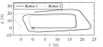
(a) true trajectory of robots 1 and 2

​

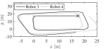
(b) true trajectory of robots 3 and 4

​ ​​​ ​ ​​​ ​​​​

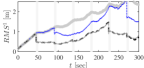
(c) robot 1

​

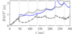
(d) robot 2

​ ​​​ ​ ​​​ ​​​​

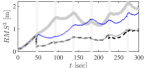
(e) robot 3

​

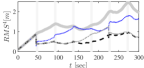
(f) robot 4

Figure 1: Simulation results for position RMS error for the measurement/communication scenario of Table I (the orientation RMS error behaves similarly and omitted for brevity). In plots (c)-(f), ultra thick gray solid line shows the RMS error for dead-recking only; black dashed line and gray dash dotted line show RMS for SA-split-EKF CL respectively in the absence and presence of link failure; and blue dotted line shows the RMS plot for the algorithm of [9].

Experimental evaluation: we tested the performance of Algorithm 1 and its robustness to message dropouts experimentally, as well. Our robotic testbed consists of a set of two overhead cameras, a computer workstation, and $4$ TurtleBot robots (see Figure 2). This testbed operates under Robot Operating System (ROS). The overhead cameras, with the help of the set of AR tags and the ArUco image processing library [22], are used to track the motion of the robots and generate a reference trajectory to evaluate the performance of the CL algorithms. The workstation serves as the server running a ROS node with the central part of the SA-split-EKF CL algorithm. Each robot has a ROS node that includes programs to propagate the local filter equations (2a), (2b) and (6a) using wheel-encoder measurements and relative-pose measurements from other robots using the onboard Kinect camera unit. To take relative-pose measurements, the Kinect camera also uses a set of AR tags and the ArUco image processing library. The robots communicate with the workstation via WiFi. The AR tags are placed on top of the TurtleBot’s rack and are arranged on a cube to provide tags in every horizontal and in top directions. The accuracy of the visual tag measurements is set to $0.03$ meter for position and to $6$ degree for orientation. For the propagation stage of every robot, the local filters of the robots apply the velocity measurement of their wheel encoders and account the noise with $50\%v$ standard deviation.

​​​

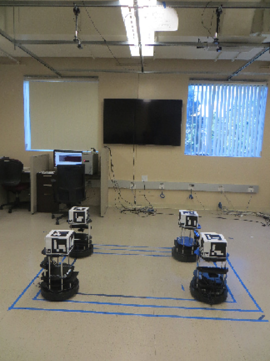
(a) The robotic testbed

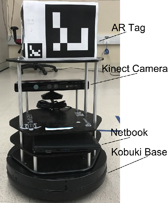
(b) Turtlebot with AR tag

Figure 2: Setup for the multi-robot test scenario showing the four TurtleBot robots. Every agent features a cube with tags that enable both the Kinect and the overhead camera to take pose measurements.

The robots move in a $2$m $\times$ $3$m area, which is the active vision zone of our overhead camera system. The robots move simultaneously in a counter clock-wise direction along a square helical path shown in Figure 2 and Figure 3. Starting each at one of the four inner corners of this helical path, marked with large green crosses on Figure 3, the robots are programmed to arrive at the next corner ahead of them at the same time. Along the edge of the track the robots use their wheel encoder measurements to propagate their motion model while, at the corners, discrete relative-measurement sequences are executed to update the local-pose estimates of the robots according to Algorithm 1. In our experiment, the relative-measurement scenario is for the robot at region $1$ to take relative measurement from the robot at region $2$, and the robot at region $2$ to take relative measurement from the robot at region $3$. The testbed works under perfect communication but we emulate message dropouts as described below. In our experiment, we execute the following four estimation filters simultaneously: (a) an overhead camera tracking to generate the reference trajectory; (b) a propagation-only filter to demonstrate the accuracy of position estimates without relative measurements; (c) an execution of the CL Algorithm 1 under a perfect communication scenario; (d) an execution of the CL Algorithm 1 under a measurement-dropout scenario. Note here that each of the CL filters (c) and (d) has its own corresponding server node on the workstation. Figure 3 depicts the result of one of our experiments. In this experiment, to emulate the message dropout, we partition our area as shown in Figure 3 into four regions and designate one of the areas, highlighted in gray, as the message-dropout zone. In the implementation that executes CL Algorithm 1 under the message-dropout scenario (CL filter (d)), the robot passing through the gray zone does not implement the update-message it receives from the server. In Figure 3, the trajectory generated by the overhead camera (the curve indicated by the black crosses) serves as our reference trajectory. As seen, as times goes by the position estimate generated by propagating the pose equations using the wheel encoder measurements (the trajectory depicted by the dotted curve) has large estimation error. In Figure 3, the location estimate of the robots via the CL Algorithm 1 under perfect-communication and message-dropout scenarios are depicted, respectively by the solid red curve and the blue dashed curve. As we can see, whenever a relative measurement is obtained, the CL algorithms improve the location accuracy of the robots. Of particular interest is the effect of CL algorithm on the position accuracy of robots when they pass through region $4$ (the shaded region on Figure 3). In our scenario described above, no relative measurement is taken by or from the robot in region $4$. However, because of maintained past correlations among the robots through the server, in the case of the perfect-communication scenario the robot in region $4$ still benefits from the relative measurement updates generated by measurements taken by other robots. Of course, in the message-dropout scenario (see the blue dashed line trajectories) such benefit is lost because the robot in region $4$ does not receive the update message from the server. However, the trajectories show the robustness of Algorithm 1 to message dropout, i.e., the robots that receive the update message from the server continue to improve their localization accuracy while the robot in region $4$ is momentarily deprived from such benefit. However, as soon as the latter reconnects and receives an update message, its accuracy improves again.

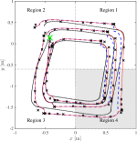
(a) robot 1

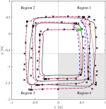
(b) robot 2

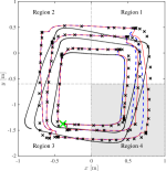
(c) robot 3

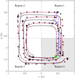
(d) robot 4

Figure 3: Trajectories of the robots under an experimental test generated by $4$ simultaneously running ROS packages, one for the overhead camera location tracking (the curve indicated by black crosses), one for the propagation only location estimate (the black dotted curve), and the other two to obtain location estimates by the the SA-split-EKF CL algorithm (Algorithm 1) under perfect communication (red solid curve) and message-dropout (dashed blue curve) scenarios. Region $4$ which is highlighted in gray is the area where we emulate the message dropout.

VI Conclusions

For a team of robots with limited computational, storage and communication resources, we proposed a server assisted distributed CL algorithm which under the perfect communication scenarios renders the same localization performance as of a joint CL using EKF. In terms of the team size, this algorithm only requires $O(1)$ storage and computational cost per robot and the main computational burden of implementing the EKF for CL is carried out by the server. We showed that this algorithm has robustness to occasional communication failure between robots and the server. Here, we discarded the measurement of the robots that fail to communicate with the server. Our future work involves utilizing these old measurements using out-of-sequence-measurement update strategies [23] when the communication link is restored between the corresponding robot and the server.

[Proof of Theorems II.1 and IV.1 ]

Proof of Theorem II.1.

Our proof is based on the mathematical induction over $k\in{\mathbb{Z}}_{\geq 0}$. Let $k=0$. Given (6) and the defined initial conditions, the right hand side of (8) results in $\!\boldsymbol{\mathbf{\Phi}}^{i}(1)\,\boldsymbol{\mathbf{\Pi}}_{i,j}(0)\,\boldsymbol{\mathbf{\Phi}}^{j}(1)\!^{\top}\!\!\!=\!\boldsymbol{\mathbf{F}}^{i}(1)\,\boldsymbol{\mathbf{0}}_{n^{i}\times n^{j}}\,\boldsymbol{\mathbf{F}}^{j}(1)\!^{\top}\!\!\!=\!\boldsymbol{\mathbf{0}}_{n^{i}\times n^{j}}$, which matches exactly the value (2c) gives for $\boldsymbol{\mathbf{P}}_{i,j}^{\mbox{-}}(1)$. Next, we validate (9) at $k=0$. When there is no relative measurement at the first step, because of (7a), (9a) and (9b) give respectively $\hat{\boldsymbol{\mathbf{x}}}^{i\mbox{+}}(1)=\hat{\boldsymbol{\mathbf{x}}}^{i\mbox{-}}(1)$ and $\boldsymbol{\mathbf{P}}^{i\mbox{+}}(1)=\boldsymbol{\mathbf{P}}^{i\mbox{-}}(1)$ which match exactly what (2d) and (2e) provide. Given (7d)-(7c) and (6b), the right hand side of (9c) reads as $\boldsymbol{\mathbf{\Phi}}^{i}(1)\,\boldsymbol{\mathbf{\Pi}}_{i,j}(1)\,\boldsymbol{\mathbf{\Phi}}^{j}(1)^{\top}=\boldsymbol{\mathbf{\Phi}}^{i}(1)\,\boldsymbol{\mathbf{\Pi}}_{i,j}(0)\,\boldsymbol{\mathbf{\Phi}}^{j}(1)^{\top}=\boldsymbol{\mathbf{0}}_{n^{i}\times n^{j}}$ which matches exactly the value  (2f) gives for $\boldsymbol{\mathbf{P}}_{i,j}^{\mbox{+}}$. On the other hand, when there is a relative measurement $a\xrightarrow{1}b$, validity of (9) follows from followings. Using (7d)-(7c), we obtain $\boldsymbol{\mathbf{\Gamma}}_{i}(1)=(\boldsymbol{\mathbf{\Pi}}_{i,b}(0){\boldsymbol{\mathbf{\Phi}}^{b}(1)}^{\top}\tilde{\boldsymbol{\mathbf{H}}}_{b}^{\top}\!+\!\boldsymbol{\mathbf{\Pi}}_{i,a}(0){\boldsymbol{\mathbf{\Phi}}^{a}(1)}^{\top}\tilde{\boldsymbol{\mathbf{H}}}_{a}^{\top})=\boldsymbol{\mathbf{0}},~{}i\in\mathcal{V}\backslash\{a,b\}$, $\boldsymbol{\mathbf{\Phi}}^{a}(1)\boldsymbol{\mathbf{\Gamma}}_{a}(1)=\boldsymbol{\mathbf{F}}^{a}(1)\boldsymbol{\mathbf{F}}^{a}(1)^{-1}\boldsymbol{\mathbf{P}}^{a\mbox{-}}(1)\tilde{\boldsymbol{\mathbf{H}}}_{a}(1)^{\top}\,{\boldsymbol{\mathbf{S}}_{a,b}}(1)^{-\frac{1}{2}}=\boldsymbol{\mathbf{K}}_{a}(1){\boldsymbol{\mathbf{S}}_{a,b}}(1)^{\frac{1}{2}}$ and $\boldsymbol{\mathbf{\Phi}}^{b}(1)\boldsymbol{\mathbf{\Gamma}}_{b}(1)=\boldsymbol{\mathbf{F}}^{b}(1)\boldsymbol{\mathbf{F}}^{b}(1)^{-1}\boldsymbol{\mathbf{P}}^{b\mbox{-}}(1)\tilde{\boldsymbol{\mathbf{H}}}_{b}(1)^{\top}\!\,{\boldsymbol{\mathbf{S}}_{a,b}}(1)^{-\frac{1}{2}}=\boldsymbol{\mathbf{K}}_{b}(1)\boldsymbol{\mathbf{S}}_{a,b}^{\frac{1}{2}}.$ Moreover, $\boldsymbol{\mathbf{\Pi}}_{i,j}(1)=\boldsymbol{\mathbf{\Pi}}_{i,j}(0)+\boldsymbol{\mathbf{\Gamma}}_{i}(1)\,\boldsymbol{\mathbf{\Gamma}}_{j}(1)=\boldsymbol{\mathbf{0}}$,  $i\in\mathcal{V}\backslash\{a,b\}$, $j\in\mathcal{V}\backslash\{i,a,b\}$. Here, we used $\boldsymbol{\mathbf{\Phi}}^{a}(1)=\boldsymbol{\mathbf{F}}^{a}(1)$, $\boldsymbol{\mathbf{\Phi}}^{b}(1)=\boldsymbol{\mathbf{F}}^{b}(1)$, $\boldsymbol{\mathbf{\Pi}}_{i,j}(0)=\boldsymbol{\mathbf{0}}$ and $\boldsymbol{\mathbf{P}}^{\mbox{-}}_{i,j}(0)=\boldsymbol{\mathbf{0}}$ for $i\in\mathcal{V}$, $j\in\mathcal{V}\backslash\{i\}$. Therefore, (9c) gives $\boldsymbol{\mathbf{P}}_{i,j}^{\mbox{+}}(1)=\boldsymbol{\mathbf{0}}$, $i\in\mathcal{V}\setminus\{a,b\},~{}j\in\mathcal{V}\backslash\{i,a,b\}$, and

$$\boldsymbol{\mathbf{P}}_{a,b}^{\mbox{+}}(1)=\!\boldsymbol{\mathbf{P}}_{b,a}^{\mbox{+}}(1)^{\top}\!=\!\boldsymbol{\mathbf{\Phi}}^{a}(1)(\boldsymbol{\mathbf{\Pi}}_{a,b}(0)\!-\!\boldsymbol{\mathbf{\Gamma}}_{a}(1)\,\boldsymbol{\mathbf{\Gamma}}_{b}(1)^{\top})\boldsymbol{\mathbf{\Phi}}^{b}(1)^{\top}$$

$$~{}=-\boldsymbol{\mathbf{\Phi}}^{a}(1)\boldsymbol{\mathbf{\Gamma}}_{a}(1)\,\boldsymbol{\mathbf{\Gamma}}_{b}(1)^{\top}\boldsymbol{\mathbf{\Phi}}^{b}(1)^{\top}=-\boldsymbol{\mathbf{K}}_{a}(1)\boldsymbol{\mathbf{S}}_{a,b}(1)\boldsymbol{\mathbf{K}}_{b}(1)^{\top},$$

which exactly matches (2f) as shown below (recall (2g)). First note that, (2f) reduces to $\boldsymbol{\mathbf{P}}_{i,j}^{\mbox{+}}(1)=\boldsymbol{\mathbf{0}}$ for $i\in\mathcal{V}\setminus\{a,b\}$ and $j\in\mathcal{V}\backslash\{i,a,b\}$. We also obtain $\boldsymbol{\mathbf{P}}_{a,b}^{\mbox{+}}(1)=\boldsymbol{\mathbf{P}}_{b,a}^{\mbox{+}}(1)^{\top}=\boldsymbol{\mathbf{P}}_{a,b}^{\mbox{-}}\!(1)-\boldsymbol{\mathbf{K}}_{a}(1)\boldsymbol{\mathbf{S}}_{a,b}(1)\boldsymbol{\mathbf{K}}_{b}(1)^{\top}=-\boldsymbol{\mathbf{K}}_{a}(1)\boldsymbol{\mathbf{S}}_{a,b}(1)\boldsymbol{\mathbf{K}}_{b}(1)^{\top}$.

Assume now that the theorem statement holds for $k$. Then at time step $k+1$, we have $\boldsymbol{\mathbf{\Phi}}^{i}(k+1)\boldsymbol{\mathbf{\Pi}}_{i,j}(k)\boldsymbol{\mathbf{\Phi}}^{j}(k+1)^{\top}=\boldsymbol{\mathbf{F}}^{i}(k+1)\boldsymbol{\mathbf{\Phi}}^{i}(k)\boldsymbol{\mathbf{\Pi}}_{i,j}(k)\boldsymbol{\mathbf{\Phi}}^{j}(k)^{\top}\boldsymbol{\mathbf{F}}^{j}(k+1)^{\top}=\boldsymbol{\mathbf{F}}^{i}(k+1)\boldsymbol{\mathbf{P}}_{i,j}^{\mbox{+}}(k)\boldsymbol{\mathbf{F}}^{j}(k+1)^{\top}=\boldsymbol{\mathbf{P}}_{i,j}^{\mbox{-}}(k+1)$, which confirms validity of (8) at $k+1$. Next, we show (9c) is correct. When there is no relative measurement at $k+1$, using (7d)-(7c) and (6b) we can write $\boldsymbol{\mathbf{\Phi}}^{i}(k+1)\boldsymbol{\mathbf{\Pi}}_{i,j}(k+1)\boldsymbol{\mathbf{\Phi}}^{j}(k+1)^{\top}=\boldsymbol{\mathbf{\Phi}}^{i}(k+1)\boldsymbol{\mathbf{\Pi}}_{i,j}(k)\boldsymbol{\mathbf{\Phi}}^{j}(k+1)^{\top}$, which confirms the correct outcome of $\boldsymbol{\mathbf{P}}_{i,j}^{\mbox{+}}(k+1)=\boldsymbol{\mathbf{P}}_{i,j}^{\mbox{-}}(k+1)$ holds at $k+1$. Next, we evaluate (9c) when robot $a$ takes a relative measurement from robot $b$ at $k+1$. First, notice that we can always write

$$\boldsymbol{\mathbf{K}}_{i}(k+1)=\boldsymbol{\mathbf{\Phi}}^{i}(k+1)\boldsymbol{\mathbf{\Gamma}}_{i}(k+1)\boldsymbol{\mathbf{S}}_{a,b}^{-\frac{1}{2}},\quad i\in\mathcal{V},$$ (A.18)

becuase

• for $i\in\mathcal{V}\backslash\{a,b\}$ (recall (7d), (8),) we have $\boldsymbol{\mathbf{\Phi}}^{i}(k\!+\!1)\boldsymbol{\mathbf{\Gamma}}_{i}(k\!+\!1)\boldsymbol{\mathbf{S}}_{a,b}^{-\frac{1}{2}}\!=\!\boldsymbol{\mathbf{\Phi}}^{i}(k\!+\!1)(\boldsymbol{\mathbf{\Pi}}_{i,b}(k){\boldsymbol{\mathbf{\Phi}}^{b}(k\!+\!1)}\!^{\top}\tilde{\boldsymbol{\mathbf{H}}}_{b}\!^{\top}\!\!\!+\!\boldsymbol{\mathbf{\Pi}}_{i,a}(k){\boldsymbol{\mathbf{\Phi}}^{a}(k\!+\!1)}^{\top}\tilde{\boldsymbol{\mathbf{H}}}_{a}\!^{\top}){\boldsymbol{\mathbf{S}}_{a,b}}\!\!^{-1}=(\boldsymbol{\mathbf{P}}_{i,b}^{\mbox{-}}(k\!+\!1)\tilde{\boldsymbol{\mathbf{H}}}_{b}^{\top}+\boldsymbol{\mathbf{P}}_{i,a}^{\mbox{-}}(k\!+\!1)\tilde{\boldsymbol{\mathbf{H}}}_{a}^{\top}){\boldsymbol{\mathbf{S}}_{a,b}}\!\!^{-1}\!=\!\boldsymbol{\mathbf{K}}_{i}(k\!+\!1)$;

• for $i=a$ (recall (7b), (8),) we have $\boldsymbol{\mathbf{\Phi}}^{i}(k+1)\boldsymbol{\mathbf{\Gamma}}_{i}(k+1)\boldsymbol{\mathbf{S}}_{a,b}^{-\frac{1}{2}}=\boldsymbol{\mathbf{\Phi}}^{a}(k+1)\big{(}\boldsymbol{\mathbf{\Pi}}_{a,b}(k){\boldsymbol{\mathbf{\Phi}}^{b}\!(k\!+\!1)}\!^{\top}\tilde{\boldsymbol{\mathbf{H}}}_{b}^{\top}\!\!\!+\!\boldsymbol{\mathbf{\Phi}}^{a}\!(k\!+\!1)^{-1}\boldsymbol{\mathbf{P}}^{a\mbox{-}}\!(k\!+\!1)\tilde{\boldsymbol{\mathbf{H}}}_{a}\!\!^{\top}\big{)}{\boldsymbol{\mathbf{S}}_{a,b}}\!\!^{-1}=\!(\boldsymbol{\mathbf{P}}_{a,b}^{\mbox{-}}(k+1)\tilde{\boldsymbol{\mathbf{H}}}_{b}\!^{\top}\!+\!\boldsymbol{\mathbf{P}}^{a\mbox{-}}(k\!+\!1)\tilde{\boldsymbol{\mathbf{H}}}_{a}^{\top}){\boldsymbol{\mathbf{S}}_{a,b}}\!\!^{-1}\!\!=\!\boldsymbol{\mathbf{K}}_{a}(k\!+\!1)$;

• for $i=b$ (recall (7c), (8),) we have $\boldsymbol{\mathbf{\Phi}}^{i}(k+1)\boldsymbol{\mathbf{\Gamma}}_{i}(k+1)\boldsymbol{\mathbf{S}}_{a,b}^{-\frac{1}{2}}=\boldsymbol{\mathbf{\Phi}}^{b}(k+1)\big{(}\boldsymbol{\mathbf{\Phi}}^{b}(k+1)^{-1}\boldsymbol{\mathbf{P}}^{b\mbox{-}}(k+1)\tilde{\boldsymbol{\mathbf{H}}}_{b}^{\top}+\!\boldsymbol{\mathbf{\Pi}}_{b,a}(k){\boldsymbol{\mathbf{\Phi}}^{a}(k+1)}^{\top}\tilde{\boldsymbol{\mathbf{H}}}_{a}^{\top}\big{)}\,{\boldsymbol{\mathbf{S}}_{a,b}}\!\!^{-1}=(\boldsymbol{\mathbf{P}}^{b\mbox{-}}(k+1)\tilde{\boldsymbol{\mathbf{H}}}_{b}^{\top}\!+\!\boldsymbol{\mathbf{P}}^{\mbox{-}}_{b,a}(k)\tilde{\boldsymbol{\mathbf{H}}}_{a}^{\top})\,{\boldsymbol{\mathbf{S}}_{a,b}}\!\!^{-1}\!=\!\boldsymbol{\mathbf{K}}_{b}(k+1)$.

Therefore, by recalling (7d)-(7c) and (6b), we can write $\boldsymbol{\mathbf{\Phi}}^{i}(k+1)\boldsymbol{\mathbf{\Pi}}_{i,j}(k+1)\boldsymbol{\mathbf{\Phi}}^{j}(k+1)^{\top}=\boldsymbol{\mathbf{\Phi}}^{i}(k+1)\boldsymbol{\mathbf{\Pi}}_{i,j}(k)\boldsymbol{\mathbf{\Phi}}^{j}(k+1)^{\top}-\boldsymbol{\mathbf{\Phi}}^{i}(k+1)\boldsymbol{\mathbf{\Gamma}}_{i}(k+1)\,\boldsymbol{\mathbf{\Gamma}}_{j}(k+1)^{\top}\boldsymbol{\mathbf{\Phi}}^{j}(k+1)^{\top}=\boldsymbol{\mathbf{P}}_{i,j}^{\mbox{-}}(k+1)-\big{(}\boldsymbol{\mathbf{\Phi}}^{i}(k+1)\boldsymbol{\mathbf{\Gamma}}_{i}(k+1)\,\boldsymbol{\mathbf{S}}_{a,b}^{-\frac{1}{2}}\big{)}\boldsymbol{\mathbf{S}}_{a,b}\,\big{(}\boldsymbol{\mathbf{\Phi}}^{j}(k+1)\boldsymbol{\mathbf{\Gamma}}_{j}(k+1)\boldsymbol{\mathbf{S}}_{a,b}^{-\frac{1}{2}}\big{)}^{\top}=\boldsymbol{\mathbf{P}}_{i,j}^{\mbox{-}}(k+1)-\boldsymbol{\mathbf{K}}_{i}(k+1)\boldsymbol{\mathbf{S}}_{a,b}\boldsymbol{\mathbf{K}}_{j}(k+1)^{\top}=\boldsymbol{\mathbf{P}}_{i,j}^{\mbox{+}}(k+1)$, which confirms validity of (9c) at $k+1$ when robot $a$ takes relative measurement from robot $b$. This completes the proof of validity of (9c) for all $k\in{\mathbb{Z}}_{\geq 0}$. Subsequently, (9a) and (9b) follow, in a straightforward manner, from (A.18) now being valid for all $k\in{\mathbb{Z}}_{\geq 0}$. ∎

Proof of Theorem IV.1.

We can obtain Kalman gain $\boldsymbol{\mathbf{K}}_{1:m}$ that minimizes $\text{Trace}(\boldsymbol{\mathbf{P}}^{\mbox{+}}(k+1))$ from $\partial\text{Trace}(\boldsymbol{\mathbf{P}}^{\mbox{+}}(k+1))/\partial\boldsymbol{\mathbf{K}}_{1:m}=\boldsymbol{\mathbf{0}}$. Let $\hat{\boldsymbol{\mathbf{x}}}_{1:m}^{\mbox{+}}=(\hat{\boldsymbol{\mathbf{x}}}^{1\mbox{+}},\cdots,\hat{\boldsymbol{\mathbf{x}}}^{m\mbox{+}})$, $\hat{\boldsymbol{\mathbf{x}}}_{m+1:N}^{\mbox{+}}=(\hat{\boldsymbol{\mathbf{x}}}^{m+1\mbox{+}},\cdots,\hat{\boldsymbol{\mathbf{x}}}^{N\mbox{+}})$. Next, we obtain $\text{Trace}(\boldsymbol{\mathbf{P}}^{\mbox{+}}(k+1))$. Given (14), we have

$$\begin{bmatrix}\begin{smallmatrix}\boldsymbol{\mathbf{x}}_{1:m}(k+1)-\boldsymbol{\mathbf{x}}_{1:m}^{\mbox{+}}(k+1)\\ \boldsymbol{\mathbf{x}}_{m+1:N}(k+1)-\boldsymbol{\mathbf{x}}_{m+1:N}^{\mbox{+}}(k+1)\end{smallmatrix}\end{bmatrix}\approx\begin{bmatrix}\begin{smallmatrix}\boldsymbol{\mathbf{e}}_{1:m}^{\mbox{+}}(k+1)\\ \boldsymbol{\mathbf{e}}_{m+1:N}^{\mbox{+}}(k+1)\end{smallmatrix}\end{bmatrix}=\!$$

$$\begin{bmatrix}\begin{smallmatrix}(\boldsymbol{\mathbf{I}}_{m}-\!\boldsymbol{\mathbf{K}}_{1:m}\bar{\boldsymbol{\mathbf{H}}})&\boldsymbol{\mathbf{0}}\\ \boldsymbol{\mathbf{0}}&\boldsymbol{\mathbf{I}}_{N-m}\end{smallmatrix}\end{bmatrix}\!\!\!\begin{bmatrix}\begin{smallmatrix}\boldsymbol{\mathbf{x}}_{1:m}(k\!+\!1)-\boldsymbol{\mathbf{x}}_{1:m}^{\mbox{-}}(k\!+\!1)\\ \boldsymbol{\mathbf{x}}_{m+1:N}(k\!+\!1)-\boldsymbol{\mathbf{x}}_{m+1:N}^{\mbox{-}}(k\!+\!1)\end{smallmatrix}\end{bmatrix}$$

$$~{}\qquad\qquad\quad\qquad+\begin{bmatrix}\begin{smallmatrix}-\boldsymbol{\mathbf{K}}_{1:m}&\boldsymbol{\mathbf{0}}\\ \boldsymbol{\mathbf{0}}&\boldsymbol{\mathbf{0}}\end{smallmatrix}\end{bmatrix}\!\!\!\begin{bmatrix}\begin{smallmatrix}\boldsymbol{\mathbf{\nu}}^{a}(k+1)\\ \boldsymbol{\mathbf{0}}\end{smallmatrix}\end{bmatrix}\!\!,$$

where $\bar{\boldsymbol{\mathbf{H}}}=\big{[}\begin{smallmatrix}\overset{1}{\boldsymbol{\mathbf{0}}}~{}~{}\overset{\cdots}{\cdots}~{}~{}\overset{a}{\tilde{\boldsymbol{\mathbf{H}}}_{a}}(k+1)~{}~{}\overset{a+1}{\boldsymbol{\mathbf{0}}}~{}~{}\overset{\cdots}{\cdots}~{}~{}\overset{b}{\tilde{\boldsymbol{\mathbf{H}}}_{b}}(k+1)~{}~{}\overset{b+1}{\boldsymbol{\mathbf{0}}}~{}~{}\overset{\cdots}{\cdots}\overset{m}{\boldsymbol{\mathbf{0}}}\end{smallmatrix}\big{]}$. Recall that $\boldsymbol{\mathbf{P}}^{\mbox{+}}(k+1)\!=\!\text{E}[\boldsymbol{\mathbf{e}}^{\mbox{+}}(k+1)\boldsymbol{\mathbf{e}}^{\mbox{+}}(k+1)^{\top}]$ which is equal to

$$\boldsymbol{\mathbf{P}}^{\mbox{+}}(k+1)=\!$$ (A.19)

$$\begin{smallmatrix}\left[\begin{array}[]{c|c}\boldsymbol{\mathbf{P}}^{\mbox{+}}_{1:m,1:m}(k+1)&\boldsymbol{\mathbf{P}}^{\mbox{+}}_{1:m,m+1:N}(k+1)\\ \hline\cr\boldsymbol{\mathbf{P}}^{\mbox{+}}_{1:m,m+1:N}(k+1)^{\top}&\boldsymbol{\mathbf{P}}^{\mbox{+}}_{m+1:N,m+1:N}(k+1)\end{array}\right]\!\end{smallmatrix}=$$

$$\!\begin{bmatrix}\begin{smallmatrix}\boldsymbol{\mathbf{K}}_{1:m}\boldsymbol{\mathbf{R}}_{a}\boldsymbol{\mathbf{K}}_{1:m}^{\top}&\boldsymbol{\mathbf{0}}_{m\times(N-m)}\\ \boldsymbol{\mathbf{0}}_{(N-m)\times m}&\boldsymbol{\mathbf{0}}_{(N-m)\times(N-m)}\end{smallmatrix}\end{bmatrix}\!+\!\begin{bmatrix}\begin{smallmatrix}(\boldsymbol{\mathbf{I}}_{m}\!-\!\boldsymbol{\mathbf{K}}_{1:m}\bar{\boldsymbol{\mathbf{H}}})\!\!\!\!\!&\boldsymbol{\mathbf{0}}\\ \boldsymbol{\mathbf{0}}&\!\!\!\boldsymbol{\mathbf{I}}_{N-m}\end{smallmatrix}\end{bmatrix}$$

$$\!\!\begin{smallmatrix}\times\left[\begin{array}[]{c|c}\boldsymbol{\mathbf{P}}^{\mbox{-}}_{1:m,1:m}(k+1)&\boldsymbol{\mathbf{P}}^{\mbox{-}}_{1:m,m+1:N}(k+1)\\ \hline\cr\boldsymbol{\mathbf{P}}^{\mbox{-}}_{m+1:N,1:m}(k+1)&\boldsymbol{\mathbf{P}}^{\mbox{-}}_{m+1:N,m+1:N}(k+1)\end{array}\right]\end{smallmatrix}\times$$

$$\!\!\begin{bmatrix}\begin{smallmatrix}(\boldsymbol{\mathbf{I}}_{m}-\boldsymbol{\mathbf{K}}_{1:m}\bar{\boldsymbol{\mathbf{H}}})^{\top}&\boldsymbol{\mathbf{0}}\\ \boldsymbol{\mathbf{0}}&\boldsymbol{\mathbf{I}}_{N-m}\end{smallmatrix}\end{bmatrix}\!\!.$$

Then, we have $\text{Trace}(\boldsymbol{\mathbf{P}}^{\mbox{+}}(k+1))=\text{Trace}(\boldsymbol{\mathbf{P}}^{\mbox{-}}_{1:m,1:m}(k+1))\!-2\,\text{Trace}(\boldsymbol{\mathbf{K}}_{1:m}\bar{\boldsymbol{\mathbf{H}}}\boldsymbol{\mathbf{P}}^{\mbox{-}}_{1:m,1:m}(k+1))+\text{Trace}(\boldsymbol{\mathbf{K}}_{1:m}(\boldsymbol{\mathbf{R}}_{a}+\bar{\boldsymbol{\mathbf{H}}}\boldsymbol{\mathbf{P}}^{\mbox{-}}_{1:m,1:m}(k+1)\bar{\boldsymbol{\mathbf{H}}}^{\top})\boldsymbol{\mathbf{K}}_{1:m}^{\top})+\text{Trace}(\boldsymbol{\mathbf{P}}^{\mbox{-}}_{m+1:N,m+1:N}(k+1))$. As a result, we have $\partial\text{Trace}(\boldsymbol{\mathbf{P}}^{\mbox{+}}(k+1))/\partial\boldsymbol{\mathbf{K}}_{1:m}=-2\,\boldsymbol{\mathbf{P}}^{\mbox{-}}_{1:m,1:m}(k+1)\bar{\boldsymbol{\mathbf{H}}}^{\top}+2\,(\boldsymbol{\mathbf{R}}_{a}+\bar{\boldsymbol{\mathbf{H}}}\boldsymbol{\mathbf{P}}^{\mbox{-}}_{1:m,1:m}(k+1)\bar{\boldsymbol{\mathbf{H}}}^{\top})\boldsymbol{\mathbf{K}}_{1:m}^{\top}=-2\,\boldsymbol{\mathbf{P}}^{\mbox{-}}_{1:m,1:m}(k+1)\bar{\boldsymbol{\mathbf{H}}}^{\top}+2\,\boldsymbol{\mathbf{S}}_{a,b}\boldsymbol{\mathbf{K}}_{1:m}^{\top}$. Therefore, the gain $\boldsymbol{\mathbf{K}}_{1:m}$ that minimizes $\text{Trace}(\boldsymbol{\mathbf{P}}^{\mbox{+}}_{1:m}(k+1))$ is $\boldsymbol{\mathbf{K}}_{1:m}=\bar{\boldsymbol{\mathbf{H}}}\boldsymbol{\mathbf{P}}^{\mbox{-}}_{1:m,1:m}(k+1)\boldsymbol{\mathbf{S}}_{a,b}^{-1}$, which equivalently expands in robot-wise components to give us (15). For the covariance update, from (A.19), we obtain

$$\boldsymbol{\mathbf{P}}^{\mbox{+}}_{1:m,1:m}(k+1)=\,(\boldsymbol{\mathbf{I}}_{m}-\boldsymbol{\mathbf{K}}_{1:m}\bar{\boldsymbol{\mathbf{H}}})\times$$ (A.20a)

$$\qquad\boldsymbol{\mathbf{P}}^{\mbox{-}}_{1:m,1:m}(k+1)(\boldsymbol{\mathbf{I}}_{m}-\boldsymbol{\mathbf{K}}_{1:m}\bar{\boldsymbol{\mathbf{H}}})^{\top}+\boldsymbol{\mathbf{K}}_{1:m}\boldsymbol{\mathbf{R}}_{a}\boldsymbol{\mathbf{K}}_{1:m}^{\top}$$

$$\quad\quad\quad\quad\quad\quad~{}~{}\,=\,\boldsymbol{\mathbf{P}}^{\mbox{-}}_{1:m,1:m}(k+1)-\boldsymbol{\mathbf{K}}_{1:m}\boldsymbol{\mathbf{S}}_{a,b}\boldsymbol{\mathbf{K}}_{1:m}^{\top},$$

$$\boldsymbol{\mathbf{P}}^{\mbox{+}}_{m+1:N,m+1:N}(k+1)=\,\boldsymbol{\mathbf{P}}^{\mbox{-}}_{m+1:N,m+1:N}(k+1),$$ (A.20b)

$$\boldsymbol{\mathbf{P}}^{\mbox{+}}_{1:m,m+1:N}(k\!+\!1)\!=\!(\boldsymbol{\mathbf{I}}_{m}\!-\!\boldsymbol{\mathbf{K}}_{1:m}\bar{\boldsymbol{\mathbf{H}}})\times$$ (A.20c)

$$\boldsymbol{\mathbf{P}}^{\mbox{-}}_{1:m,m+1:N}(k\!+\!1)\!=\!\Big{(}\boldsymbol{\mathbf{I}}_{m}\!\!-\!\begin{bmatrix}\begin{smallmatrix}\boldsymbol{\mathbf{K}}_{1}\\ \vdots\\ \boldsymbol{\mathbf{K}}_{m}\end{smallmatrix}\end{bmatrix}\!\!\!\Big{[}\overset{1}{\boldsymbol{\mathbf{0}}}~{}\,\overset{\cdots}{\cdots}~{}\,\overset{a}{\tilde{\boldsymbol{\mathbf{H}}}_{a}}(k)~{}\,\overset{a+1}{\boldsymbol{\mathbf{0}}}~{}$$

$$\qquad\quad\,\overset{\cdots}{\cdots}~{}\,\overset{b}{\tilde{\boldsymbol{\mathbf{H}}}_{b}}(k)~{}\,\overset{b+1}{\boldsymbol{\mathbf{0}}}~{}\,\overset{\cdots}{\cdots}\overset{m}{\boldsymbol{\mathbf{0}}}\Big{]}\!\Big{)}\boldsymbol{\mathbf{P}}^{\mbox{-}}_{1:m,m+1:N}(k+1)=$$

$$\Big{(}\!\boldsymbol{\mathbf{I}}_{m}\!-\!\begin{bmatrix}\begin{smallmatrix}\boldsymbol{\mathbf{K}}_{1}\boldsymbol{\mathbf{S}}_{a,b}\boldsymbol{\mathbf{S}}_{a,b}^{-1}\\ \vdots\\ \boldsymbol{\mathbf{K}}_{m}\boldsymbol{\mathbf{S}}_{a,b}\boldsymbol{\mathbf{S}}_{a,b}^{-1}\end{smallmatrix}\end{bmatrix}\Big{[}\overset{1}{\boldsymbol{\mathbf{0}}}~{}\,\overset{\cdots}{\cdots}~{}\,\overset{a}{\tilde{\boldsymbol{\mathbf{H}}}_{a}}(k)$$

$$\qquad\quad~{}\,\overset{a+1}{\boldsymbol{\mathbf{0}}}~{}\,\overset{\cdots}{\cdots}~{}\,\overset{b}{\tilde{\boldsymbol{\mathbf{H}}}_{b}}(k)~{}\,\overset{b+1}{\boldsymbol{\mathbf{0}}}~{}\,\overset{\cdots}{\cdots}\overset{m}{\boldsymbol{\mathbf{0}}}\Big{]}\!\Big{)}\boldsymbol{\mathbf{P}}^{\mbox{-}}_{1:m,m+1:N}(k+1),$$

where

$$\boldsymbol{\mathbf{P}}^{\mbox{-}}_{1:m,m+1:N}(k\!+\!1)\!=\!\begin{bmatrix}\begin{smallmatrix}\boldsymbol{\mathbf{P}}^{\mbox{-}}_{1,m+1}(k\!+\!1)\!&\cdots&\!\boldsymbol{\mathbf{P}}^{\mbox{-}}_{1,N}(k\!+\!1)\\ \vdots&\cdots&\vdots\\ \boldsymbol{\mathbf{P}}^{\mbox{-}}_{m,m+1}(k\!+\!1)\!&\cdots&\!\boldsymbol{\mathbf{P}}^{\mbox{-}}_{m,N}(k\!+\!1)\end{smallmatrix}\end{bmatrix}$$

Recalling the definition of the pseudo-gains (17), then (A.20) results in (16a) and (16b). ∎

[Sequential updating for multiple measurements] For multiple synchronized measurements, we use the sequential updating procedure. Let $\mathcal{V}_{\text{A}}(k)$ denote the set of the robots that have made an exteroceptive measurement at time $k$, $\mathcal{V}_{\text{\text{B}}}^{i}(k)$ denote the landmark robots of robot $i\in\mathcal{V}_{\text{A}}(k)$, and $\mathcal{V}_{\text{A,B}}(k)$ represent the set of all landmark robots and the robots that have taken relative measurements. Then the total number of relative measurements is $n_{s}=\sum\nolimits_{i=1}^{|\mathcal{V}_{\text{A}}(k)|}|\mathcal{V}_{\text{\text{B}}}^{i}(k)|$. Recall that in sequential updating, the measurements are processed one by one, starting with using the first measurement to update the predicted estimate and error covaraince matrix, and proceeding with next measurement to update the current updated state estimate and error measurements. By straightforward substitution, the sequential updating procedure in Split-EKF CL variables, starting with $\hat{\boldsymbol{\mathbf{x}}}^{i\mbox{+}}(k+1,0)=\hat{\boldsymbol{\mathbf{x}}}^{i\mbox{-}}(k+1)$, $\boldsymbol{\mathbf{P}}^{i\mbox{+}}(k+1,0)=\boldsymbol{\mathbf{P}}^{i\mbox{-}}(k+1)$, $i\in\mathcal{V}$, and $\boldsymbol{\mathbf{P}}_{i,l}^{\mbox{+}}(k+1,0)=\boldsymbol{\mathbf{P}}_{i,l}^{i\mbox{-}}(k+1)$ for $l\in\mathcal{V}\backslash\{i\}$, reads as (starting at $j=1$),

$$\text{for}~{}a\in\mathcal{V}_{\text{A}}(k+1),$$

$$\quad\text{for}~{}b\in\mathcal{V}^{a}_{\text{B}}(k+1),\quad\quad\quad$$

$$\!\hat{\boldsymbol{\mathbf{x}}}^{i\mbox{+}}(k\!+\!1,j)\!=\hat{\boldsymbol{\mathbf{x}}}^{i\mbox{-}}(k\!+\!1,j-1)+$$

$$\quad\quad\qquad\qquad\qquad\quad\boldsymbol{\mathbf{\Phi}}^{i}(k\!+\!1)\boldsymbol{\mathbf{\Gamma}}_{i}(k\!+\!1,j)\bar{\boldsymbol{\mathbf{r}}}^{a}(k\!+\!1,j),$$

$$\!\boldsymbol{\mathbf{P}}^{i\mbox{+}}(k\!+\!1,j)\!=\boldsymbol{\mathbf{P}}^{i\mbox{-}}\!(k\!+\!1,j-1)-$$

$$\qquad\quad\quad\quad\boldsymbol{\mathbf{\Phi}}^{i}(k+1)\boldsymbol{\mathbf{\Gamma}}_{i}(k+1,j)\boldsymbol{\mathbf{\Gamma}}_{i}\!^{\top}(k+1,j)\boldsymbol{\mathbf{\Phi}}^{i}(k+1)\!^{\top}\!,$$

$$\!\boldsymbol{\mathbf{P}}_{i,l}^{\mbox{+}}(k\!+\!1,j)\!=\boldsymbol{\mathbf{\Phi}}^{i}(k\!+\!1)\,\boldsymbol{\mathbf{\Pi}}_{i,l}(k\!+\!1,j-1)\,\boldsymbol{\mathbf{\Phi}}^{l}(k\!+\!1)\!^{\top}\!\!,$$

$$\quad~{}~{}~{}j\leftarrow j+1,$$

where $\boldsymbol{\mathbf{\Pi}}_{i,j}(k+1,0)=\boldsymbol{\mathbf{\Pi}}_{i,j}(k)$, $\boldsymbol{\mathbf{\Pi}}_{i,j}(k+1,j)=\boldsymbol{\mathbf{\Pi}}_{i,j}(k+1,j-1)+\boldsymbol{\mathbf{\Gamma}}_{i}(k+1,j)\,\boldsymbol{\mathbf{\Gamma}}_{j}(k+1,j)^{\top}$. Here, $\boldsymbol{\mathbf{\Gamma}}_{i}(k+1,j)$ is calculated from (7d)-(7c) wherein $\boldsymbol{\mathbf{S}}_{a,b}$ at each $j$ is calculated from (II) using $\hat{\boldsymbol{\mathbf{x}}}^{\mbox{-}}(k+1)=\hat{\boldsymbol{\mathbf{x}}}^{\mbox{+}}(k+1,j-1)$ and $\boldsymbol{\mathbf{P}}^{\mbox{-}}(k+1)=\boldsymbol{\mathbf{P}}^{\mbox{+}}(k+1,j-1)$. Consequently, $\bar{\boldsymbol{\mathbf{r}}}^{a}(k+1,j)=\boldsymbol{\mathbf{S}}_{a,b}(k+1,j)^{-\frac{1}{2}}\boldsymbol{\mathbf{r}}^{a}(k\!+\!1,j)$. The update at time $k+1$ is $\hat{\boldsymbol{\mathbf{x}}}^{i\mbox{+}}(k+1)=\hat{\boldsymbol{\mathbf{x}}}^{i\mbox{+}}(k+1,n_{s})$, $\boldsymbol{\mathbf{P}}^{i\mbox{+}}(k+1)=\boldsymbol{\mathbf{P}}^{i\mbox{+}}(k+1,n_{s})$, and $\boldsymbol{\mathbf{P}}_{i,l}^{\mbox{+}}(k+1)=\boldsymbol{\mathbf{P}}_{i,l}^{\mbox{+}}(k+1,n_{s})$, $i\in\mathcal{V}$, $l\in\mathcal{V}\backslash\{i\}$.

Notice that we can represent the final updated variables as

$$\hat{\boldsymbol{\mathbf{x}}}^{i\mbox{+}}(k+1,n_{s})=\hat{\boldsymbol{\mathbf{x}}}^{i\mbox{-}}(k\!+\!1,0)+$$ (B.21a)

$$\quad\quad\boldsymbol{\mathbf{\Phi}}^{i}(k\!+\!1)\sum\nolimits_{j=1}^{n_{s}}\boldsymbol{\mathbf{\Gamma}}_{i}(k\!+\!1,j)\bar{\boldsymbol{\mathbf{r}}}^{a}(k\!+\!1,j),$$

$$\boldsymbol{\mathbf{P}}^{i\mbox{+}}(k+1,n_{s})=\boldsymbol{\mathbf{P}}^{i\mbox{-}}\!(k\!+\!1,0)-$$ (B.21b)

$$\quad\quad\!\boldsymbol{\mathbf{\Phi}}^{i}(k\!+\!1)\Big{(}\sum\nolimits_{j=1}^{n_{s}}\boldsymbol{\mathbf{\Gamma}}_{i}(k\!+\!1,j)\boldsymbol{\mathbf{\Gamma}}_{i}^{\top}(k\!+\!1,j)\Big{)}\boldsymbol{\mathbf{\Phi}}^{i}(k\!+\!1)\!^{\top}\!,$$

$$\boldsymbol{\mathbf{P}}_{i,l}^{\mbox{+}}(k\!+\!1,n_{s})=$$ (B.21c)

$$\quad\quad\boldsymbol{\mathbf{\Phi}}^{i}(k+1)\Big{(}\sum\nolimits_{j=1}^{n_{s}}\,\boldsymbol{\mathbf{\Pi}}_{i,l}(k+1,j-1)\,\Big{)}\boldsymbol{\mathbf{\Phi}}^{l}(k+1)^{\top}.$$

Algorithm 2 Server’s sequential updating procedure for multiple in-network measurement at time $k+1$

1:Initialization ($j=0$): server obtains the following information from each robot $a\in\mathcal{V}_{\text{A}}(k+1)$ and all of its landmarks $b\in\mathcal{V}_{\text{B}}^{a}(k+1)$,

$$\textsl{Landmark-message}^{a}=\Big{(}\boldsymbol{\mathbf{z}}_{a,b},\hat{\boldsymbol{\mathbf{x}}}^{a\mbox{-}}(k+1),\boldsymbol{\mathbf{P}}^{b\mbox{-}}(k+1),\boldsymbol{\mathbf{\Phi}}^{a}(k+1)\Big{)},$$

$$\textsl{Landmark-message}_{a}^{b}=\Big{(}\hat{\boldsymbol{\mathbf{x}}}^{b\mbox{-}}(k+1),\boldsymbol{\mathbf{P}}^{b\mbox{-}}(k+1),\boldsymbol{\mathbf{\Phi}}^{b}(k+1)\Big{)}.$$

The server initializes the following variables

$$\hat{\boldsymbol{\mathbf{x}}}^{\mbox{+}i}(k\!+\!1,0) =\hat{\boldsymbol{\mathbf{x}}}^{\mbox{-}i}(k\!+\!1),~{}\hat{\boldsymbol{\mathbf{P}}}^{\mbox{+}i}(k\!+\!1,0)=\boldsymbol{\mathbf{P}}^{\mbox{-}i}(k\!+\!1),~{}\forall i\in\bar{\mathcal{V}}(k\!+\!1),$$

$$\boldsymbol{\mathbf{\Pi}}_{i,l}(k\!+\!1,0) =\boldsymbol{\mathbf{\Pi}}_{i,l}(k),i\in\mathcal{V}\backslash\{N\},~{}l\in\{i\!+\!1,\cdots,N\}.$$

Iteration $j$: server proceeds with the following calculations.

2:for $a\in\mathcal{V}_{\text{A}}(k+1)$ do

3:    for $b\in\mathcal{V}_{\text{B}}^{a}(k+1)$ do

4:       Server calculates $\tilde{\boldsymbol{\mathbf{H}}}_{a}$, $\tilde{\boldsymbol{\mathbf{H}}}_{b}$ and $\boldsymbol{\mathbf{r}}^{a}$ using $\hat{\boldsymbol{\mathbf{x}}}^{\mbox{-}a}(k+1)=\hat{\boldsymbol{\mathbf{x}}}^{\mbox{+}a}(k+1,j-1)$ and $\hat{\boldsymbol{\mathbf{x}}}^{\mbox{-}b}(k+1)=\hat{\boldsymbol{\mathbf{x}}}^{\mbox{+}b}(k+1,j-1)$. Then, using these measurement matrices and $\hat{\boldsymbol{\mathbf{P}}}^{\mbox{-}a}(k+1)=\hat{\boldsymbol{\mathbf{P}}}^{\mbox{+}a}(k+1,j-1)$, $\hat{\boldsymbol{\mathbf{P}}}^{\mbox{-}b}(k+1)=\hat{\boldsymbol{\mathbf{P}}}^{\mbox{+}b}(k+1,j-1)$ and $\boldsymbol{\mathbf{\Pi}}_{a,b}(k)=\boldsymbol{\mathbf{\Pi}}_{a,b}(k+1,j-1)$, server calculates $\boldsymbol{\mathbf{S}}_{a,b}$ from (II) and subsequently $\bar{\boldsymbol{\mathbf{r}}}^{a}(k+1,j)=(\boldsymbol{\mathbf{S}}_{a,b}(k+1,j))^{-\frac{1}{2}}\boldsymbol{\mathbf{r}}^{a}(k+1,j)$ and $\boldsymbol{\mathbf{\Gamma}}_{i}(k+1,j)$ from (7d)-(7c) for $i\in\mathcal{V}$. Next, server updates the state and the covariance of all the robots in $i\in{\mathcal{V}_{\text{A,B}}}(k+1)$ as follows

$$\hat{\boldsymbol{\mathbf{x}}}^{\mbox{+}i}(k\!+\!1,j)=\hat{\boldsymbol{\mathbf{x}}}^{\mbox{+}i}(k\!+\!1,j)\!+\!\boldsymbol{\mathbf{\Phi}}^{i}(k\!+\!1)\,\boldsymbol{\mathbf{\Gamma}}_{i}(k\!+\!1,j)\,\bar{\boldsymbol{\mathbf{r}}}^{a}\!(k\!+\!1,j),$$ (B.22a)

$$\boldsymbol{\mathbf{P}}^{\!\mbox{+}i}\!(k\!+\!1,j)\!=\!\boldsymbol{\mathbf{P}}^{\!\mbox{+}i}(\!k\!+\!1,\!j)\!-\!\boldsymbol{\mathbf{\Phi}}^{\!i}(k\!+\!1)\boldsymbol{\mathbf{\Gamma}}_{i}(k\!+\!1,\!j)\!\boldsymbol{\mathbf{\Gamma}}_{i}(k\!+\!1,\!j)\!^{\top}\!\!\boldsymbol{\mathbf{\Phi}}^{i}\!(k\!+\!1)^{\!\top}\!\!.$$ (B.22b)

It also updates $\boldsymbol{\mathbf{\Pi}}_{i,l}$ for $i\in\mathcal{V}\backslash\{N\},~{}l\in\{i+1,\cdots,N\}$ as follows

$$\boldsymbol{\mathbf{\Pi}}_{i,l}(k+1,j)=\boldsymbol{\mathbf{\Pi}}_{i,l}(k+1 ,j-1)-\boldsymbol{\mathbf{\Gamma}}_{i}(k+1,j)\boldsymbol{\mathbf{\Gamma}}_{l}(k+1,j)^{\top},\quad$$

$$\text{if~{}}(i,l)\not\in\mathcal{V}_{\text{missed}}(k+1)\times\mathcal{V}_{\text{missed}}(k+1).$$

5:       $j\leftarrow j+1$

6:    end for

7:end for

8:server sets $\boldsymbol{\mathbf{\Pi}}_{i,l}(k+1)=\boldsymbol{\mathbf{\Pi}}_{i,l}(k+1,n_{s})$, where $n_{s}=\sum_{a\in\mathcal{V}_{\text{A}}(k+1)}|\mathcal{V}_{\text{\text{B}}}^{a}(k+1)|$.

9:server broadcasts the following update messages for robot $i\in\mathcal{V}$

$$\textsl{update-message}^{i}=\, \Big{(}\sum\nolimits_{j=1}^{n_{s}}\!(\boldsymbol{\mathbf{\Gamma}}_{i}(k+1,j)\bar{\boldsymbol{\mathbf{r}}}^{a}(k+1,j)),$$ (B.23)

$$~{}~{}\sum\nolimits_{j=1}^{n_{s}}\!(\boldsymbol{\mathbf{\Gamma}}_{i}(k+1,j)\boldsymbol{\mathbf{\Gamma}}_{i}(k+1,j)^{\top})\Big{)}.$$

One can expect that the updating order must not dramatically change the results (cf.  [19, page 104] and references therein). Here, we assume that the server has a pre-specified sequential-updating-order guideline, which indicates the priority order for implementing the measurement update. To implement sequential updating procedure, the robots making measurements inform the server and indicate to server what their landmark robots are., i.e., the server knows $\mathcal{V}_{\text{A}}(k+1)$ and $\mathcal{V}_{\text{\text{B}}}^{i}(k+1)$’s, and sorts both of these sets according to it’s sequential-updating-order guideline. The server collects all the landmark messages (• ‣ 3) of the robots in $\mathcal{V}_{\text{A,B}}(k+1)$. We use the compact representation (B.21) of the sequential updating procedure to develop a partially decentralized implementation which requires only one update message broadcast from the server, see Algorithm 2. Note that in this implementation, the server should create a local copy of the state estimate and the error covariance equations of the robots in ${\mathcal{V}_{\text{A,B}}}(k+1)$ (see. (B.22)), because these updates are needed to compute $\boldsymbol{\mathbf{S}}_{a,b}$ and other intermediate variables. An alternative implementation is also possible where the update message for every robot $i\in\mathcal{V}_{\text{A},\text{B}}(k+1)$ is

$$\textsl{update-message}^{i}=\Big{(}(\boldsymbol{\mathbf{\Phi}}^{i})^{-1}(\hat{\boldsymbol{\mathbf{x}}}^{\mbox{+}i}(k+1,n_{s})-\hat{\boldsymbol{\mathbf{x}}}^{\mbox{-}i}(k+1)),$$

$$\quad\qquad-\!(\boldsymbol{\mathbf{\Phi}}^{i})^{-1}(\boldsymbol{\mathbf{P}}^{\mbox{+}i}(k+1,n_{s})\!-\!\boldsymbol{\mathbf{P}}^{\mbox{-}i}(k+1))(\boldsymbol{\mathbf{\Phi}}^{i})^{-T}\Big{)}.$$

instead of (B.23). This is because the server already has computed the update state estimates and the corresponding covariances of robot $i\in{\mathcal{V}_{\text{A,B}}}(k+1)$ as part of partial updating procedure, i.e, $\hat{\boldsymbol{\mathbf{x}}}^{\mbox{+}i}(k+1)=\hat{\boldsymbol{\mathbf{x}}}^{\mbox{+}i}(k+1,n_{s})$, and $\boldsymbol{\mathbf{P}}^{\mbox{+}i}(k+1)=\boldsymbol{\mathbf{P}}^{\mbox{+}i}(k+1,n_{s})$.

References

- [1] J. Leonard and H. F. Durrant-Whyte, “Mobile robot localization by tracking geometric beacons,” IEEE Transactions on Robotics and Automation, vol. 7, pp. 376–382, June 1991.
- [2] G. Dissanayake, P. Newman, H. F. Durrant-Whyte, , S. Clark, and M. Csorba, “A solution to the simultaneous localization and map building (SLAM) problem,” IEEE Transactions on Robotics and Automation, vol. 17, no. 3, pp. 229–241, 2001.
- [3] S. I. Roumeliotis, Robust mobile robot localization: from single-robot uncertainties to multi-robot interdependencies. PhD thesis, University of Southern California, 2000.
- [4] A. Howard, M. J. Matarić, and G. S. Sukhatme, “Mobile sensor network deployment using potential fields: A distributed scalable solution to the area coverage problem,” in Int. Conference on Distributed Autonomous Robotic Systems, (Fukuoka, Japan), pp. 299–308, June 2002.
- [5] N. Trawny, S. I. Roumeliotis, and G. B. Giannakis, “Cooperative multi-robot localization under communication constraints,” in IEEE Int. Conf. on Robotics and Automation, (Kobe, Japan), pp. 4394–4400, May 2009.
- [6] A. Bahr, M. R. Walter, and J. J. Leonard, “Consistent cooperative localization,” in IEEE Int. Conf. on Robotics and Automation, (Kobe, Japan), pp. 8908–8913, May 2009.
- [7] P. O. Arambel, C. Rago, and R. K. Mehra, “Covariance intersection algorithm for distributed spacecraft state estimation,” in American Control Conference, (Arlington, VA), pp. 4398–4403, 2001.
- [8] L. C. Carrillo-Arce, E. D. Nerurkar, J. L. Gordillo, and S. I. Roumeliotis, “Decentralized multi-robot cooperative localization using covariance intersection,” in IEEE/RSJ Int. Conf. on Intelligent Robots & Systems, (Tokyo, Japan), pp. 1412–1417, 2013.
- [9] H. Li and F. Nashashibi, “Cooperative multi-vehicle localization using split covariance intersection filter,” IEEE Intelligent Transportation Systems Magazine, vol. 5, no. 2, pp. 33–44, 2013.
- [10] D. Marinescu, N. O’Hara, and V. Cahill, “Data incest in cooperative localisation with the common past-invariant ensemble kalman filter,” in IEEE Int. Conf. on Information Fusion, (Istanbul, Turkey), pp. 68–76, 2013.
- [11] L. Luft, T. Schubert, S. I. Roumeliotis, and W. Burgard, “Recursive decentralized collaborative localization for sparsely communicating robots,” in Robotics: Science and Systems, (AnnArbor, Michigan), June 2016.
- [12] S. E. Webster, J. M. Walls, L. L. Whitcomb, and R. M. Eustice, “Decentralized extended information filter for single-beacon cooperative acoustic navigation: Theory and experiments,” IEEE Transactions on Robotics, vol. 29, no. 4, pp. 957–974, 2013.
- [13] S. S. Kia, S. Rounds, and S. Martínez, “Cooperative localization for mobile agents: a recursive decentralized algorithm based on Kalman filter decoupling,” IEEE Control Systems Magazine, vol. 36, no. 2, pp. 86–101, 2016.
- [14] S. I. Roumeliotis and G. A. Bekey, “Distributed multirobot localization,” IEEE Transactions on Robotics and Automation, vol. 18, no. 5, pp. 781–795, 2002.
- [15] E. D. Nerurkar, S. I. Roumeliotis, and A. Martinelli, “Distributed maximum a posteriori estimation for multi-robot cooperative localization,” in IEEE Int. Conf. on Robotics and Automation, (Kobe, Japan), pp. 1402–1409, May 2009.
- [16] K. Y. K. Leung, T. D. Barfoot, and H. H. T. Liu, “Decentralized localization of sparsely-communicating robot networks: A centralized-equivalent approach,” IEEE Transactions on Robotics, vol. 26, no. 1, pp. 62–77, 2010.
- [17] S. S. Kia, S. Rounds, and S. Martínez, “Cooperative Localization under message dropouts via a partially decentralized EKF scheme,” in IEEE Int. Conf. on Robotics and Automation, (Seattle, WA, USA), pp. 5977–5982, May 2015.
- [18] C. T. Leondes, ed., Advances in Control Systems Theory and Application, vol. 3. New York: Academic Press, 1966.
- [19] Y. Bar-Shalom, P. K. Willett, and X. Tian, Tracking and Data Fusion, a Handbook of Algorithms. Storts, CT, USA: YBS Publishing, 2011.
- [20] S. S. Kia and S. Martinez, “A partially decentralized ekf scheme for cooperative localization over unreliable communication links,” 2016. https://arxiv.org/abs/1608.00609.
- [21] J. L. Crassidis and J. L. Junkins, Optimal Estimation of Dynamic Systems. Chapman & Hall/CRC, 2 ed., 2011.
- [22] R. M. Salinas and B. Magyar, “ArUco ROS library.” http://wiki.ros.org/aruco.
- [23] Y. Bar-Shalom, H. Chen, and M. Mallick, “One-step solution for the multistep out-of-sequence- measurement problem in tracking,” IEEE Transactions on Aerospace and Electronic Systems, vol. 40, no. 1, pp. 27–37, 2004.