Stability Aspects of Wormholes in Gravity
Abstract
We study radial perturbations of a wormhole in -gravity to determine regions of stability. We also investigate massive and massless particle orbits and tidal forces in this space-time for a radially infalling observer.
I Introduction
Wormholes are intriguing solutions to Einstein’s theory of general relativity, though their physical existence is highly contested. Wormholes are shortcut paths between different parts of spacetime and have long served as a theoretical laboratory for exploring exotic phenomena in general relativity Morris:1988tu ; Morris:1988cz ; Visser:1995cc . Wormhole solutions are found by specifying the desired spacetime through sewing together two separate spacetimes with black hole geometries. This procedure determines the type of energy-momentum tensor necessary to support such a solution and typically describes “exotic” types of mass and energy. There are longstanding discussions regarding the viability of constructing wormhole solutions in standard general relativity. Surprisingly, wormholes in a certain modification of general relativity, namely solutions of gravity, exist without the need for exotic matter Duplessis:2015xva . gravity has recently gained attention due to the discovery of new spherically symmetric solutions in the regime Kehagias:2015ata , including black hole solutions in general quadratic gravity Lu:2015cqa . One of the intriguing features of gravity is, unlike in General Relativity, it is possible to have non-trivial Ricci tensor even when .
In this paper we study stability properties of the aforementioned gravity wormhole solutions. We identify regions in parameter space which yield a stable wormhole by studying radial perturbations. In addition, we search for stable orbits around these wormholes and determine whether an astrophysical probe in an universe could possibly traverse such a wormhole without experiencing destructive tidal forces. The present work explores these questions by adapting previous stability inquiries for wormholes in standard general relativity such as those discussed in Poisson:1995sv .
We begin in section II by reviewing the wormhole construction found in Duplessis:2015xva , and in section III we determine the junction conditions needed in gravity. In section IV we discuss the criteria for a stable wormhole and find regions in parameter space where stability holds. Section V examines the stability of orbits around the stable wormhole construction, and section VI determines the tidal forces encountered by a radially infalling observer passing through the wormhole. We conclude in section VII.
II Wormhole Construction
Consider the wormhole solution to gravity. is a requirement for this vacuum solution. The metric is
| (1) |
where we define
| (2) |
Here, is the radius of the wormhole throat and is the metric on the unit two-sphere. The constant sets the minimal throat radius, and the full form of can be found in the Appendix of Duplessis:2015xva . If , then and the space is asymptotically Minkowski. For large we have and the space is similar to Reissner-Nordström. (We shall not need the definitions of and , but they can be found in Duplessis:2015xva .) Therefore, allowing the throat at to have time dependence, we have the relations
| (3) | |||||
| (4) | |||||
| (5) |
From equation (1) we find
| (6) |
along with the timelike Killing vector
| (7) |
and the four-velocity
| (8) |
The extrinsic curvature is then given by
| (9) |
One can perform the derivative, which gives
| (10) |
It can be seen that this is equivalent to using the replacements
| (11) | |||||
| (12) | |||||
| (13) |
in the found from the metric
| (14) |
This makes sense when directly comparing the metrics given in equations (1) and (14). Similar replacements can be made to recover and . We find
| (15) |
III gravity junction conditions
We have the energy-momentum on the throat given in terms of the extrinsic curvature
| (16) |
where
| (17) |
and and are given by the jump discontinuity equations for the extrinsic curvature
| (18) | |||||
| (19) |
with being the trace of the extrinsic curvature
| (20) |
In the case of our metric (1) we have the following relations of importance
| (21) | |||||
| (22) | |||||
| (23) | |||||
| (24) | |||||
| (25) | |||||
| (26) | |||||
| (27) |
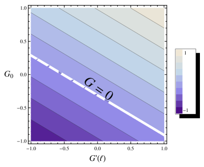
IV Stability
Apparently models are all subject to the junction condition Eiroa:2015hrt in order for there to be no jump discontinuity between the two spaces. In our case this becomes
| (28) |
where we will be interested in the static case where . This leads to
| (29) |
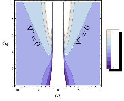
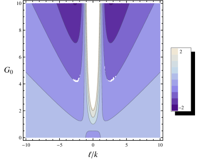
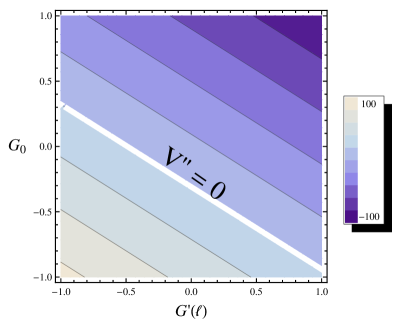
Defining the potential
| (30) |
we find
| (31) |
Stability is then given by the condition .
V Orbits around the wormhole
Beginning with the explicit form of the metric
| (32) |
we examine equatorial orbits with , where we have the geodesic equations
| (33) | |||||
| (34) | |||||
| (35) |
The equation can be written as
| (36) |
Which leads to the constant of motion
| (37) |
The equation can be written as
| (38) |
This gives the constant
| (39) |
We also know that the quantity
| (40) |
is a constant along the path parameterized by . If then this is for a massive particle, and it is always equal to zero for a massless particle. Following Carroll:1997ar we will call this constant , which then gives
| (41) | |||||
| (42) |
This can be written as
| (43) |
with the effective potential defined as
| (44) |
One can then find the stable orbits for and .
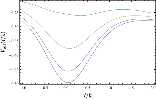
Figure 5 demonstrates there exists a region of orbital stability due to the presence of a minimum for the effective potential, and it is just on the positive side as is lowered towards zero ( is roughly where the minimum value occurs as ). Unstable orbits are seen to exist when maxima of the effective potential are present.
VI Tidal Forces
By looking at the difference in acceleration between two neighboring points we are able to determine the tidal forces that a radially infalling observer will experience. To do this we use the equation for the tidal acceleration previously found in Duplessis:2015xva given as
| (45) |
where is the separation distance between the two points, measured by our infalling observer, and is the four-velocity.
The Riemann tensors, which determine the tidal forces for the metric (1) are found in Duplessis:2015xva , and here we reproduce them in terms of the variable
| (46) | |||
| (47) |
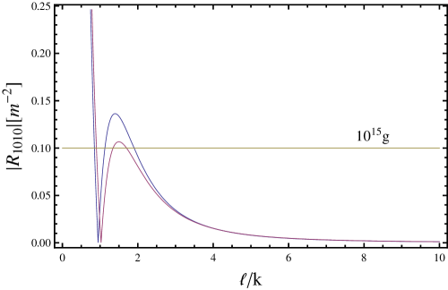
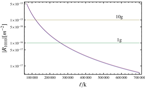
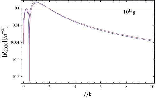
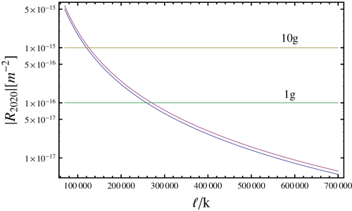
In order to determine if the infalling observer will survive the journey through the wormhole, we now examine the tidal forces in the range of parameter values previously found to produce a stable wormhole configuration. As a benchmark, and following the traditional treatment found in Morris:1988cz , we will utilize the acceleration standard of the gravitational acceleration, (9.8m/s2 in SI units), at the surface of the Earth.
The absolute values of the Riemann tensors are translated to factors of as shown in figures (6-9). In these figures, the parameter set to meter implies that the values give in meters. Unsurprisingly, for very small values, equivalently small wormhole throats, the tidal forces produced are immense, but decline precipitously with increasing , reaching values sustainable by humans (or human-built spacecraft) at only a few hundred km for these parameter values.
VII Discussion and Conclusion
While gravity may not correspond to physical reality, it provides a testing ground where we can find analytic solutions and study their corresponding stability. (The case has been made for the physical significance of conformal gravity Mannheim:2011ds , which is also quadratic in the curvature.) Hence the solutions and properties thereof discussed here may be relevant to more physically well motivated general theories of quadratic gravity. Here we have found stability conditions for radially perturbed wormholes in gravity with that do not require exotic matter. Properties of stable particle orbits in these solutions then give us hints of what we may expect to find in classes of more general theories that are quadratic in curvature.
VIII Acknowledgements
J.B.D. thanks Dr. and Mrs. Sammie W. Cosper at the University of Louisiana at Lafayette, and the Louisiana Board of Regents for support. S.C.W. would like to thank Eric M. Schlegel for useful discussions.
References
- (1) B. P. Abbott et al. [LIGO Scientific and Virgo Collaborations], Phys. Rev. Lett. 116, 061102 (2016) [arXiv:1602.03837 [gr-qc]].
- (2) M.S. Morris, K.S. Thorne, and U. Yurtsever, Phys. Rev. Lett. 61, 1446 (1988).
- (3) M.S. Morris and K.S. Thorne, Am. J. Phys. 56, 395 (1988).
- (4) M. Visser, “Lorentzian Wormholes: From Einstein to Hawking”, (1995) AIP Series in Computational and Applied Mathematical Physics, Woodbury, USA.
- (5) F. Duplessis and D. Easson, Phys. Rev. D 92, 043516 (2015) [arXiv:1506.00988].
- (6) A. Kehagias, C. Kounnas, D. Lust, and A. Riotto, JHEP 1505, 143 (2015) [arXiv:1502.04192].
- (7) H. Lu, A. Perkins, C.N. Pope, and K.S. Stelle, Phys. Rev. Lett. 114, 171601 (2015) [arXiv:1502.01028].
- (8) E. F. Eiroa and G. Figueroa Aguirre, Eur. Phys. J. C 76, 132 (2016) [arXiv:1511.02806 [gr-qc]].
- (9) E. Poisson and M. Visser, Phys. Rev. D 52, 7318 (1995) [gr-qc/9506083].
- (10) S. M. Carroll, “Lecture notes on general relativity,” gr-qc/9712019.
- (11) P. D. Mannheim, Found. Phys. 42, 388 (2012) [arXiv:1101.2186 [hep-th]].