We study a topological superconductor island with spatially separated Majorana modes coupled to multiple normal metal leads by single electron tunneling in the Coulomb blockade regime. We show that low-temperature transport in such Majorana island is carried by an emergent charge- boson composed of a Majorana mode and an electron from the leads. This transmutation from Fermi to Bose statistics has remarkable consequences. For noninteracting leads, the system flows to a non-Fermi liquid fixed point, which is stable against tunnel couplings anisotropy or detuning away from the charge-degeneracy point. As a result, the system exhibits a universal conductance at zero temperature, which is a fraction of the conductance quantum, and low-temperature corrections with a universal power-law exponent. In addition, we consider Majorana islands connected to interacting one-dimensional leads, and find different stable fixed points near and far from the charge-degeneracy point.
Electron Teleportation in Multi-Terminal Majorana Islands:
Statistical Transmutation and Fractional Quantum Conductance
pacs:
74.20.Rp, 74.20.Mn, 74.45.+cMajorana modes are an unusual type of quasiparticles in topological superconductors, consisting of localized electron and hole excitations in an equal superposition kitaev ; read ; wilczek . The presence of spatially separated Majorana modes in a macroscopic topological superconductor gives rise to degenerate ground states that are locally indistinguishable and topologically protected. In a mesoscopic superconductor island with Majoranas (a Majorana island), however, these ground states partially split into two charge-parity sectors with the total number of electrons being even and odd respectively; this energy splitting is unrelated to Majorana mode hybridization, but comes from the charging energy and can be tuned by a gate voltage fu ; xu . This tunability enables electric control of Majoranas as well as new schemes of braiding and quantum computation based on mesoscopic topological superconductor devices heck ; hassler ; grosfeld ; alicea ; hyart ; terhal ; vijay ; landau .
The interplay between Majorana modes and charging energy gives rise to a variety of topological quantum phenomena at the mesoscopic scale. One example is transport through a topological superconductor island with two spatially separated Majorana modes, each connected to a normal metal lead by electron tunneling fu ; egger ; glazman . Theory fu predicts that an unusual resonant tunneling process involving two distant Majoranas gives rise to a phase-coherent charge- transport dubbed electron teleportation, exhibiting a conductance peak when the island is at a charge-degeneracy point. In a recent groundbreaking experiment marcus on proximitized nanowires under a magnetic field —a promising platform for topological superconductivity sarma ; oreg ; kouwenhoven ; weizmann , -periodic zero-bias conductance through the superconducting island has been observed in the Coulomb blockade regime, providing experimental support for electron teleportation via Majorana modes.
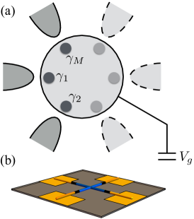
In this work, we study multi-terminal charge transport through a Majorana island connected with leads, each tunnel coupled to a Majorana zero mode, as shown in Fig. 1. We assume these Majoranas are far apart and have vanishing wavefunction hybridization. The charge on the island is tuned by a gate voltage. This type of Majorana islands have recently been fabricated marcus2 ; marcus3 and attracted considerable interest.
Our study is also motivated by recent theoretical breakthroughs BeriCooper ; AltlandEgger ; Beri ; Affleck13 ; AltlandBeryEggerTsvelik14 ; Tsvelik ; numerics ; ZazunovAltlandEgger14 ; Eriksson14a ; Eriksson14 ; Kashuba15 ; Pikulin16 ; Meidan16 ; Plugge16 , especially the seminal works of Béri-Cooper BeriCooper and Altland-Egger AltlandEgger , predicting a “topological Kondo effect” in the Coulomb valley regime where the charge of the topological superconductor island is fixed. Under this condition, the Majorana degrees of freedom are constrained to be in a given fermion parity sector and collectively form a impurity “spin”, which interacts with bosonic excitations in the leads. Remarkably, this interaction gives rise to a non-Fermi-liquid fixed point without fine tuning. However, since the Kondo temperature is exponentially small, the intriguing phenomena associated with the topological Kondo fixed point is only accessible at very low temperature numerics .
Our work focuses on charge transport in multi-terminal Majorana islands in the vicinity of the charge-degeneracy point, which until now has not been studied. At this point, the charge on the island fluctuates between and as electrons tunnel in and out of it. Consequently, the conductance at high temperature exhibits a Coulomb blockade peak on resonance, and the Majorana degrees of freedom are unconstrained but correlate with the charge parity fu ; xu . Since charging energy permits only two charge states on the island, tunneling events at different leads are interrelated.
As we show, due to high-order tunneling processes that build up quantum coherence, the system flows from the unstable weak-tunneling regime to the strong-coupling regime. We find that the strong-coupling limit of Majorana islands connected with electron leads is described by a non-Fermi liquid fixed point, which is stable against gate voltage detuning away from the charge-degeneracy point and anisotropy of tunnel couplings between the island and the leads. The zero-temperature conductance at this fixed point is universal and a fraction of the conductance quantum,
| (1) |
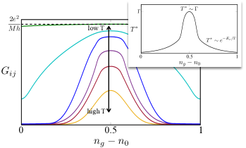
where relates the voltage on lead to the current in lead via the relation . Furthermore, the low-temperature correction to the conductance has a power-law temperature dependence with a universal exponent . Importantly, at the charge-degeneracy point, the crossover from high-temperature Coulomb blockade regime to the universal conductance Eq. (1) occurs at a temperature which is parametrically higher than the Kondo temperature in the Coulomb valley regime, see Fig.2. This greatly facilitates experimental observation of the non-Fermi liquid behavior and the universal conductance associated with electron teleportation in multi-terminal Majorana islands.
The Majorana nature of zero modes in the island is essential for the interesting physics described here. As we will show explicitly, Majoranas bind with electrons in the leads to create a new type of emergent particle—a charge- boson, which governs conduction through the island at low temperature. Because of this transmutation from Fermi to Bose statistics, a Majorana island connected with electron leads becomes equivalent to a particle interacting with bosonic reservoirs and undergoing quantum Brownian motion. This mapping then allows us to completely solve the problem of Majorana islands using a known strong-weak coupling duality YiKane .
Model.– Our multi-terminal Majorana island setup, shown in Fig. 1, is described by the Hamiltonian . The superconducting island is capacitively coupled to a gate which determines its charging energy and average occupancy as
| (2) |
Here is the electron number operator of the island. Importantly, due to the presence of zero-energy Majorana modes, the topological superconductor island admits an odd number of electrons on equal footing with an even number of electrons, without paying the energy cost of the superconducting gap (which is assumed to be the largest energy scale). Hence, the electron number is allowed to be either even or odd.
The island is coupled to the leads via single-electron tunneling described by fu
| (3) |
where creates an electron at the end of lead . are Majorana mode operators with the defining property
| (4) |
These Majorana modes are assumed to be far apart without direct coupling. The superconducting phase is conjugate to the electron number , with the commutation relation , so that changes the number of electrons in the island by . As a single electron tunnels in (out of) the island from (to) the leads, the tunneling operator Eq. (3) simultaneously flips the fermion parity of the island—which is encoded in Majorana degrees of freedom—and changes the charge on the island by .
We specialize to the case where dominates over both the temperature and the level broadening induced by coupling to leads , where is the density of states at the leads. Then, for the range of gate voltages corresponding to , only two charge states with and are relevant at low energy. We denote these two charge states by a pseudo-spin , and project the full Hamiltonian to the low-energy Hilbert space to obtain
| (5) |
where is the energy difference of the two charge states.
At high temperatures (yet lower than ), the conductance through the Majorana island exhibits a resonance peak as the gate voltage is swept across the charge-degeneracy point . Near this point and to leading order in tunnel coupling, the conductance peak is described by conventional sequential tunneling through an impurity level heck :
| (6) |
Coherent tunneling processes due to the Majorana modes manifest themselves in higher-order corrections in , and thus the crossover into the strong-coupling limit occurs at (see Fig. 2).
Statistical Transmutation.– To obtain the multi-terminal conductance at low temperature requires a non-perturbative strong-coupling analysis. First, without loss of generality, we model the noninteracting electrons in the leads as chiral fermions moving in infinite one-dimensional wires:
| (7) |
where at different leads anticommute, for .
We note that the tunneling operator shown in Eqs. (3) and (5) involves a product of an electron operator ( or ) and the self-adjoint Majorana operator . Such bilinear operators defined at different leads are bosonic and mutually-commuting,
| (8) |
for . This all-commuting condition allows us to bosonize into independent chiral boson fields:
| (9) |
Details of this bosonization procedure can be found in the appendix.
After bosonization the imaginary-time action describing the leads is given by:
| (10) |
and the tunneling term at becomes
| (11) |
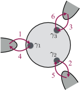
We have thus made an exact transformation mapping the problem of electron tunneling between a Majorana island and leads to a problem of boson hopping between an impurity level and reservoirs. This transformation is enabled by the presence of Majorana modes, which bind with electrons in the leads to form charge- bosons. To appreciate the importance of Majorana-enabled statistical transmutation, it is instructive to compare and contrast teleportation through Majorana islands with resonant tunneling through a single-particle energy level in a quantum dot. In both cases, the charge on the island or the dot fluctuates between two values differing by . Consider the sequence of successive tunneling events shown in Fig. 3 that exchanges two electrons on lead 1 and 3 via lead 2. The amplitude of this exchange process in a perturbative expansion in powers of the tunneling operator is negative for resonant tunneling in a quantum dot as expected for such free fermion problem. However, by a straightforward calculation using Eq. (5), one finds this amplitude is positive for teleportation in Majorana islands, showing that the effective charge carrier here is a boson. This comparison explains why the bosonized action for Majorana islands, Eq. (11), does not apply to resonant tunneling through an energy level; the latter problem involves Klein factors necessary for keeping track of electron’s Fermi statistics Nayak . We note that exchange processes are present only for setups with more than two leads. Therefore, electron teleportation in two-terminal Majorana islands fu is a special case where the effect of statistical transmutation is nulled.
Mapping to quantum Brownian motion.– We start the strong-coupling analysis by studying Majorana islands at the charge-degeneracy point and with equal tunnel couplings to all leads: . The bosonized action in Eqs. (10) and (11) is then equivalent to the action of quantum Brownian motion (QBM) of a particle in a periodic potential, as shown by Yi and Kane YiKane . To see this mapping, we integrate out the degrees of freedom away from in the leads to obtain a -dimensional action in terms of the boson phase fields , given by where
| (12) |
describes the leads, and
| (13) |
describes the tunneling between the leads and the island. Here is a -dimensional vector whose -th component is and other components are all zero, so that . We have included the normalization factor in Eq. (13) so that the scaling dimension of is equal to (for more details see Appendix).
We now identify as the momentum of a particle coupled to a dissipative bath. The number of charges carriers in the leads —which is conjugate to —corresponds to the particle’s coordinate . For small , the action describes QBM of this particle in a strong periodic potential, whose minima are located at . Specifically, determines the amount of dissipation, and , being a translation operator, generates a small probability of particle hopping between two adjacent potential minima connected by the lattice vector .
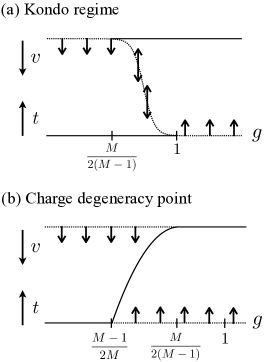
In our setup, the sum of all charges on the leads may only fluctuate by 1 due to charge conservation and the restriction of two allowed charge states and on the island. This implies that the Brownian particle is only allowed to hop on two adjacent lattice planes perpendicular to the direction . For , the potential minima of the Brownian particle form a corrugated honeycomb lattice, consisting of two triangular sublattices, as illustarted in Fig. 4. For , the particle hops on the generalization of corrugated honeycomb lattices in dimensions. The two sublattices correspond to , hence the particle hopping described by Eq. (13) alternates between the two sublattices.
For noninteracting electron leads, the hopping operator Eq. (13) has a scaling dimension given by , which is relevant at the disconnected fixed point . Thus the strong potential limit of QBM, described in terms of particle hopping between deep potential minima, is unstable and flows under RG to a different fixed point.
To identify this new fixed point, we first note that before integrating out degrees of freedom in the leads, a new term is generated in the RG process. The perturbative RG equations for the two coupling constants and are:
| (14) |
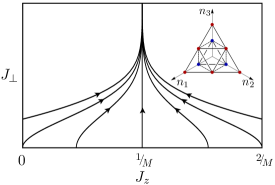
The resulting RG flow, plotted in Fig. 4, shows that , even with initial value of , flows to a Toulouse-like point in which . At this point, a unitary transformation eliminates the term from the action, similar to the analysis of Ref. YiKane . After performing the transformation, the hopping operator, Eq. (13), becomes
| (15) |
where the vectors are all orthogonal to and have the length . Importantly, the total charge field which corresponds to the motion of the Brownian particle along the direction, disappears from . As a result, the motion along is decoupled from the motion in the perpendicular direction, which is spanned by the remaining linearly independent vectors appearing in . Therefore, independent of the bare coupling constant , the system flows to the Toulouse limit with an action that is equivalent to QBM on a -dimensional honeycomb lattice.
The hopping between deep potential minima of the honeycomb lattice has a scaling dimension given by , which is smaller than for all , and thus is a relevant operator. As a result, the hopping amplitude grows, or equivalently the periodic potential weakens in the RG process. Next, we consider the limit of vanishing periodic potential, or QBM in free space. We analyze its stability against applying a periodic potential with the same periodicity as the original honeycomb lattice YiKane . Such a potential can be decomposed into Fourier components: , where is the reciprocal lattice vector defined by for any Bravais lattice vector of the honeycomb lattice. The scaling dimension of the component of the perturbation is given by (see Appendix). The shortest reciprocal-lattice vector is of length . Therefore, the periodic potential is marginal for , and irrelevant for . As argued by Yi and Kane YiKane , the contrasting stability in the limit of strong and weak potential implies that the periodic potential flows to zero in the RG process, leading to QBM in free space as the infrared fixed point.
We now turn to Majorana islands detuned away from the charge-degeneracy point and/or having unequal coupling to the leads. In the QBM formulation, the deviation from makes the two sublattices of the honeycomb lattice inequivalent. Unequal tunnel couplings described by make the honeycomb lattice spatially anisotropic. Both perturbations correspond to deformations of the honeycomb lattice that lower its crystal symmetry but does not alter its periodicity. As such, they are irrelevant at the free QBM fixed point as shown by our stability analysis. We thus conclude that the strong-coupling limit of Majorana islands connected with noninteracting electron leads is a non-Fermi liquid fixed point that maps to QBM in free space and is stable against asymmetric coupling to leads and gate voltage detuning away from the charge-degeneracy point.
Universal conductance and low-temperature corrections. The isotropy of QBM in free space implies that at the infrared fixed point, all off-diagonal components of the multi-terminal conductance matrix are equal: for . Current conservation then implies that . To determine , let us consider the following setup: we apply a voltage on the first lead, on the second lead, and for all other leads. By definition, the resulting current is
| (16) |
while in all other leads. Finding the current for this particular voltage setup will then yield , thus the entire matrix . The voltage couples to the charges on lead , and hence corresponds to adding a linear potential to the coordinate of the Brownian particle . The uniform force field in the direction and the coupling to the dissipative bath, give rise to a nonzero steady-state velocity in this direction. Since QBM in free space is spatially isotropic and direction independent, the steady-state velocity is independent of spatial dimensionality , and hence so is the current . For it was shown fu that a Majorana island with equal tunnel couplings to two leads maps to resonant electron tunneling, for which . Therefore, equating the known result for and Eq. (16) we obtain for all , yielding the universal multi-terminal conductance in Eq. (1). It is interesting to note that in the limit , the conductance which determines the total current through the island approaches , which is identical to the conductance from resonant Andreev reflection from a single Majorana mode in a grounded superconductor. This is consistent with the expectation that coupling the island to a large number of leads makes it effectively grounded.
At finite but low temperature, corrections to the conductance are governed by the leading irrelevant operator at the infrared fixed point. In the QBM formulation, this operator corresponds to adding a weak honeycomb potential, which has the scaling dimension . This gives rise to a universal power-law correction to the conductance at low temperature,
| (17) |
where is a constant of order . The temperature depends strongly on the gate voltage: near the charge-degeneracy point is significantly higher than in the Kondo regime . Consequently, coherence effects become important at higher temperatures for , and the conductance approaches its zero-temperature universal value faster (see Fig. 2).
Kondo regime– When the gate voltage is tuned to the Coulomb valley (), the charge on the island is fixed to an integer . As a result, electrons can no longer hop into or out of the island. Instead, virtual tunneling processes give rise to an effective exchange interaction that transfers charge between the leads while switching the state of Majoranas within a fermion parity sector given by . This Kondo-type interaction can also be derived from our model, Eq. (5), via second-order perturbation theory in , which yields BeriCooper
| (18) |
where are generators satisfying the Clifford algebra, and the Kondo coupling is .
As shown by Béri Beri , this Kondo problem of bosonic nature directly maps to QBM on a triangular lattice. This mapping can also be understood in our formulation: a large adds a strong sublattice potential to the corrugated honeycomb lattice, so that the Brownian particle hops between sites on the low-energy sublattice via virtual transitions through the high-energy sublattice. Importantly, the hopping operator in the Kondo regime is marginally relevant and sets the length of the triangular lattice vector to be . Analysis of Majorana islands in the Kondo regime Beri reveals that for noninteracting leads the strong-coupling fixed point also maps to QBM in free space, which is the same as the fixed point we found in the vicinity of (see also Appendix). Thus, we conclude that despite having significantly different conductance in the high-temperature Coulomb peak and Coulomb valley regime, the system exhibits the universal conductance Eq. (1) at , independent of the gate voltage. Our result generalizes Ref.Beri where the conductance was found in the Kondo regime. However, as we show below, the Coulomb peak and Coulomb valley regime of a Majorana island flow to different infrared fixed points for repulsive interactions in the leads.
Interacting leads– The QBM formulation provides a unified framework for analyzing Majorana islands both in the vicinity of the charge-degeneracy point and in the Kondo regime. Although up to here we have considered noninteracting electron leads, the generalization to the interacting case is straightforward. To study interaction effects, we only need to identify the change in the lengths of the direct and reciprocal lattice vectors, given by and , where is the Luttinger parameter YiKane . Therefore, in the Kondo regime (), arbitrarily weak repulsive interactions make irrelevant, so that the limit of decoupled Majorana island and leads is stable against weak tunnel couplings. As the couplings increase above a critical value, the system undergoes a quantum phase transition AltlandEgger ; Beri into the strong-coupling fixed point (see Fig. 5).
In contrast, near the charge-degeneracy point, electron tunneling into the Majorana island remains a relevant operator over a finite range of interaction strengths. Since and , we obtain that for , the system flows from the unstable weak-tunneling to the stable strong-coupling fixed point. For stronger repulsive interactions a stable fixed point occurs at intermediate coupling strengths (see Fig. 5).
To conclude, our work predicts a set of remarkable transport phenomena in multi-terminal Majorana islands in the vicinity of the charge-degeneracy point, including a universal fractional quantum conductance at zero temperature, and its universal power-law correction at low temperature. Observation of such phenomena will clearly demonstrate the Majorana nature of zero modes in a superconductor island, defined by the operator algebra Eq. (4) and acting as a charge-neutral Fermi-Bose transformer.
Acknowledgements: We thank Ian Affleck, Moshe Goldstein, Charlie Kane, Charlie Marcus and Michal Papaj for helpful discussions. This work is supported by David and Lucile Packard Foundation (LF), Israel Science Foundation Grant No. 1243/13, and the Marie Curie CIG Grant No. 618188 (ES), as well as the the Minerva Foundation (KM).
Appendix A Detailed study of the phase diagram
In the main text we described the mapping of Majorana islands coupled to leads onto a QBM model. Here we elaborate on the various steps of the derivation and the analysis of the phase digram (Fig. 5). We start with bosonization of the leads and integration of all degrees of freedom away from . The resulting effective action describes a particle subject to a periodic potential, and coupled to a dissipative bath. Within this QBM model we calculate the scaling dimensions of various allowed perturbations, and study the weak- and strong-tunneling limits near the charge-degeneracy point and in the Kondo regime.
A.1 Bosonization
We start the bosonization procedure by mapping the model system described above onto a spin chain. For this purpose, we describe the leads as chains of fermions
| (19) |
where the lattice constant is set to unity and the hopping parameter is fixed to reproduce the density of states in the leads . The creation (annihilation) operator at the boundary site is identified with the boundary field operator (). In general, the standard Jordan-Wigner transformation that maps one-dimensional fermions onto a spin chain fails for a system of semi-infinite wires joined at a single point. When the one-dimensional wires are coupled to the Majorana island, we can define commuting spin operators as a product of electron operators in the leads and the corresponding Majorana mode operators:
| (20) |
Correspondingly, the Hamilton can be expressed in terms of -spin chains, all connected at the origin to the spin operator of the island:
| (21) |
In this description of the system, the Majorana operators disappear from the Hamiltonian, manifesting the Bose statistics of the charge carriers in the leads.
Next we express the spin operators in each chain in terms of left () and right () moving chiral modes , where . However, we find it more convenient to describe each lead as an infinite chain , and express the spin operators in term of a single chiral mode:
| (22) |
where . The chiral operators obey the commutation relations , and the conjugate operators can be identified as the electron density operators . This is because changes the total charge by , and similarly shifts the phase by . The imaginary-time action of the leads, corresponding to the first term in Eq. (21), can be written in terms of the phase fields as
| (23) | ||||
Here, is the inverse temperature, and is the Fermi velocity.
The scaling dimension of the spin operators is obtained from the zero-temperature correlation function of the field as
| (24) | ||||
From the action Eq. (23), we get that
| (25) |
and .
Up to here, we considered free electrons in the leads. To generalize the derivation to interacting leads, we introduce the Luttinger parameter into the action:
| (26) | ||||
Here () corresponds to repulsive (attractive) interactions. Consequently, the zero-temperature correlation function
| (27) |
and the scaling dimension of the spin operators is . Furthermore, the definition of the conjugate fields is also -dependent, , and the density operator becomes .
In the derivation of the action given by Eq. (26) as well as of the properties of we followed Ref. vonDelft . An alternative approach would be to perform the bosonization with the non-chiral operators and (see for example Ref. Giamarchi ) and use the relations:
| (28) | ||||
Here () is the left (right) chiral operator. The left- and right-chiral fields are connected through the transformation .
finally, we turn to the coupling term between the leads and the Majorana island, second term in Eq. (21). Using the expressions for the spin lowering and raising operators in terms of the chiral fields, the tunneling Hamiltonian becomes
| (29) |
A.2 Boundary Action
The next step in the mapping onto QBM is to integrate out the degrees of freedom away from . For this purpose, we use the Fourier decomposition of the fields:
| (30) |
and the corresponding action:
| (31) |
Here, are the Matsubara frequencies. The field at the boundary () is obtained by integrating over momentum
| (32) |
To find the boundary action , we have to calculate the correlation function :
| (33) |
The action for the boundary field:
| (34) |
coincides with the expression given in Eq. (12) when and . Eq. (34) describes a particle subject to a classical friction term CL (Ohmic dissipation). Thus, the particle exhibits Brownian motion in an -dimensional space, where the field is its momentum along the -axis.
In the QBM framework, tunneling between the leads and the Majorana island is encoded in terms of the form . Therefore, to analyze the phase diagram it is important to find the scaling dimension of such terms. Setting in Eq. (24), we find the scaling dimensions of to be
| (35) |
This expression is needed for the analysis of the RG flow for the QBM in the weak-tunneling (strong periodic potential) regime.
For the strong-tunneling limit, we need to find the scaling dimensions of terms of the form that shift by . Previously, we saw that a shift of the phase in an infinite lead is generated by the density operator . On the boundary, we note that the operator satisfies the desired commutation relations:
| (36) |
The definition of the density operator, allows us to rewrite this operator in terms of the phase as . We note that in the strong-tunneling limit, has a finite expectation value, and correspondingly (for formulation of the boundary condition in terms of the non-chiral operators see Ref. Chamon ). This property reflects the fact that each electron that comes from is transferred to the Majorana island. As a result,
| (37) |
we find that scaling dimension of is
| (38) |
A.3 RG flow diagram near the charge-degeneracy point
The bosonized description of a Majorana island coupled to leads given in Eq. (26) and the corresponding boundary action in Eq. (34) allow us to analyze the phase diagram of the system. To follow the derivation in the main text, we assume equal coupling constants to all leads and that the gate voltage is tuned to the charge-degeneracy point, . The starting point of the calculation is the full Hamiltonian before integrating out fluctuations away from :
| (39) |
Although the bare Hamiltonian does not include the term, such a term is generated in the RG process. In the previous sections we showed that the scaling dimension of the (bare) tunneling operator is , however, it is expected to change in the RG process. To find the renormalized scaling dimension of the tunneling term, we rewrite the above Hamiltonian in the following form:
| (40) |
The -term can be eliminated from the Hamiltonian by the unitary transformation:
| (41) |
Under this transformation , and the Hamiltonian becomes:
| (42) | ||||
Specifically, for the center-of-mass boson field drops out from the tunneling term. Since the flow of stops at , the system reaches a new (Toulouse-like) fixed point.
At the fixed point, we integrate out the degrees of freedom away from , and write the boundary action as:
| (43) |
where is the -th component of the vector . Thus, in the Toulouse-like fixed point the action describes QBM of a particle that is subject to a periodic potential in an dimensional space spanned by . From Eq. (35) we find that the scaling dimension of the tunneling term is given by
| (44) |
For free electrons in the leads (), the scaling dimension of the tunneling term is relevant. Therefore, the weak-tunneling regime is unstable, and flows to infinity. At this fixed point the lattice potential vanishes, and the particle can move freely, i.e., charge strongly fluctuates between the leads. Correspondingly, the potential for is maximal and the field is locked to one of its minima.
To analyze the stability of this new fixed point we note that the symmetry allowed perturbations are of the form
| (45) |
where is a reciprocal vector of the lattice spanned by . This kind of terms restore the lattice potential that vanished in the RG flow. Equivalently, such terms describe tunneling between minima of the potential for , and they tend to decouple the leads from the Majorana island, i.e., to pin the charge. The scaling dimension of the perturbation in Eq. (45) was calculated in the previous section (see Eq. (39)). To find the reciprocal lattice vector, we use the relation for any Bravais lattice vector . For the dimensional lattice defined by , the Bravais vectors are . Correspondingly, the shortest reciprocal lattice vectors are:
| (46) |
and the scaling dimension of the tunneling operator on the reciprocal lattice is
| (47) |
Therefore, the leading perturbation is irrelevant for free leads.
For interacting leads, the tunneling term in Eq. (44) is relevant for , and the periodic potential term in Eq. (47) is relevant for . Therefore, for the system flows to the strong-tunneling (vanishing potential) fixed point, while the strong potential (decoupled leads and island) fixed point is stable for . As shown in Fig. 5, a stable intermediate fixed point appears for .
A.4 RG flow diagram in the Kondo regime
When the gate voltage is tuned far from , charge fluctuations in the island are gapped. As a result, electrons can only hop between the leads via virtual transitions through the island, and the effective action becomes:
| (48) | ||||
Where . Here, no new terms are generated in the RG process, and the center-of-mass boson does not appear in the tunneling term. Therefore to obtain the flow diagram in the Kondo regime, we follow the steps introduced in the previous section after eliminating the term (starting at Eq (43)). The boundary action can be written as
| (49) |
where . From Eq. (35), we find that the scaling dimension of the tunneling operator is . As a result, the tunneling term is marginally relevant for free leads and the system flows to the weak-potential limit. In the presence of arbitrarily weak repulsive interactions, the tunneling term is irrelevant AltlandEgger and, for not too strong bare tunnel couplings, the leads decouple from the island.
Interestingly, in the Kondo limit are the Bravais vectors of the lattice near the charge-degeneracy point (see discussion below Eq. (45)). Near the charge-degeneracy point, however, the lattice is defined by a basis vector in additional to the Bravais vectors. This point is illustrated in Fig. 4 where the QBM near is on a honeycomb lattice, while in the Kondo regime, the QBM is confined to a plane of constant total charge, and the periodic potential is triangular. As a result, the reciprocal lattice vectors in both cases are identical, and so is the scaling dimension of the leading operator in the strong-tunneling limit, Eq. (47). We conclude that for noninteracting leads, the strong-tunneling fixed points are the same in the vicinity and far from . However, only near the charge-degeneracy point the fixed point remains stable in the presence of weak repulsive interactions.
References
- (1) A. Kitaev, Ann. Phys. (N.Y.) 303, 2 (2003).
- (2) N. Read and D. Green, Phys. Rev. B. 61, 10267 (2000).
- (3) F. Wilczek, Nat. Phys. 5, 614 (2009).
- (4) L. Fu, Phys. Rev. Lett. 104, 056402 (2010).
- (5) C. Xu, and L. Fu, Phys. Rev. B. 81, 134435 (2010).
- (6) F. Hassler, A. R. Akhmerov, C. W. J. Beenakker, New J. Phys. 13, 095004 (2011).
- (7) B. van Heck, A. R. Akhmerov, F. Hassler, M.Burrello, and C. W. J. Beenakker, New J. Phys. 14, 035019 (2012).
- (8) B. M. Terhal, F. Hassler, and D. P. DiVincenzo, Phys. Rev. Lett. 108, 260504 (2012).
- (9) T. Hyart, B. van Heck, I. C. Fulga, M. Burrello, A. R. Akhmerov, and C. W. J. Beenakker, Phys. Rev. B. 88, 035121 (2013).
- (10) E. Ginossar, E. Grosfeld, Nat. Commun. 5, 4772 (2014).
- (11) S. Vijay, T. H. Hsieh, and L. Fu, Phys. Rev. X. 5, 041038 (2015).
- (12) D. Aasen et al, arXiv:1511.05153
- (13) L. A. Landau, S. Plugge, E. Sela, A. Altland, S. M. Albrecht, and R. Egger, Phys. Rev. Lett. 116, 050501 (2016).
- (14) A. Zazunov, A. Levy Yeyati, and R. Egger, Phys. Rev. B. 84, 165440 (2011).
- (15) B. van Heck, R.M. Lutchyn, and L.I. Glazman, arXiv:1603.08258
- (16) S. M. Albrecht, A. P. Higginbotham, M. Madsen, F. Kuemmeth, T. S. Jespersen, J. Nygård, P. Krogstrup, and C. M. Marcus, Nature 531, 206 (2016).
- (17) R. M. Lutchyn, J. D. Sau, and S. Das Sarma, Phys. Rev. Lett. 105, 077001 (2010).
- (18) Y. Oreg, G. Refael, and F. von Oppen, Phys. Rev. Lett. 105, 177002 (2010).
- (19) V. Mourik, K. Zuo, S. M. Frolov, S. R. Plissard, E. P. A. M. Bakkers, and L. P. Kouwenhoven, Science 336, 1003 (2012).
- (20) A. Das, Y. Ronen, Y. Most, Y. Oreg, M. Heiblum, and H. Shtrikman, Nat. Phys. 8, 887 (2012).
- (21) P. Krogstrup et al, Nat. Mat. 14, 400 (2015).
- (22) C. M. Marcus, private communication
- (23) B. Béri, and N. Cooper, Phys. Rev. Lett. 109, 156803 (2012).
- (24) A. Altland, and R. Egger, Phys. Rev. Lett. 110, 196401 (2013).
- (25) B. Béri, Phys. Rev. Lett. 110, 216803 (2013).
- (26) I. Affleck, and D. Giuliano, J. Stat. Mech. 2013 P06011 (2013).
- (27) A. Altland, B. Béri, R. Egger, and A. M. Tsvelik, J. Phys. A. 47, 265001 (2014).
- (28) A. Altland, B. Béri, R. Egger, and A. M. Tsvelik, Phys. Rev. Lett. 113, 076401 (2014).
- (29) M. R. Galpin, A. K. Mitchell, J. Temaismithi, D. E. Logan, B. Béri, N. R. Cooper, Phys. Rev. B. 89, 045143 (2014).
- (30) A. Zazunov, A. Altland, and R. Egger, New J. Phys. 16, 015010 (2014).
- (31) E. Eriksson, A. Nava, C. Mora, and R. Egger, Phys. Rev. B. 90, 245417 (2014).
- (32) E. Eriksson, C. Mora, A. Zazunov, and R. Egger, Phys. Rev. Lett. 113, 076404 (2014).
- (33) O. Kashuba and C. Timm, Phys. Rev. Lett. 114, 116801 (2015).
- (34) D. I. Pikulin, Y. Komijani, and I. Affleck, Phys. Rev. B. 93, 205430 (2016).
- (35) D. Meidan, A. Romito, and P. W. Brouwer, Phys. Rev. B. 93, 125433 (2016).
- (36) S. Plugge, A. Zazunov, E. Eriksson, A. M. Tsvelik, and R. Egger, Phys. Rev. B. 93, 104524 (2016).
- (37) H. Yi, and C. L. Kane, Phys. Rev. B. 57 R5579 (1998).
- (38) C. Chamon, M. Oshikawa, and I. Affleck, Phys. Rev. Lett. 91 206403 (2003); J. Stat. Mech. 602 P02008 (2006).
- (39) C. Nayak, M. P. A. Fisher, A. W. W. Ludwig, and H. H. Lin, Phys. Rev. B. 59 15694 (1999).
- (40) C. Kane, and M. P. A. Fisher, Phys. Rev. B. 46, 15233 (1992).
- (41) J. von Delft, and H. Schoeller, Annal. Phys. 7 225 (1998).
- (42) T. Giamarchi, Quantum physics in one dimension (Carendon, Oxford, 2003).
- (43) A. O. Caldeira, and A. J. Leggett, Phys. Rev. Lett. 46, 211 (1981).