Compact stars in $f(R,\mathcal{T})$ gravity

Abstract

In the present paper we generate a set of solutions describing the interior of a compact star under $f(R,\mathcal{T})$ theory of gravity which admits conformal motion. An extension of general relativity, the $f(R,\mathcal{T})$ gravity is associated to Ricci scalar $R$ and the trace of the energy-momentum tensor $\mathcal{T}$. To handle the Einstein field equations in the form of differential equations of second order, first of all we adopt the Lie algebra with conformal Killing vectors (CKV) which enable one to get solvable form of such equations and second we consider the equation of state (EOS) $p=\omega\rho$ with $0<\omega<1$ for the fluid distribution consisting of normal matter, $\omega$ being the EOS parameter. We therefore analytically explore several physical aspects of the model to represent behaviour of the compact stars such as - energy conditions, TOV equation, stability of the system, Buchdahl condition, compactness and redshift. It is checked that the physical validity and the acceptability of the present model within the specified observational constraint in connection to a dozen of the compact star candidates are quite satisfactory.

1 Introduction

Though Einstein’s general theory of relativity has always proved to be very fruitful for uncovering so many hidden mysteries of Nature, yet the evidence of late-time acceleration of the Universe and the possible existence of dark matter has imposed a fundamental theoretical challenge to this theory Ri1998 ; Perl1999 ; Bern2000 ; Hanany2000 ; Peebles2003 ; Paddy2003 ; clifton2012 . As a result, several modified theories on gravitation have been proposed from time to time. Among all these theories, a few of them, namely $f(R)$ gravity, $f(T)$ gravity and $f(R,\mathcal{T})$ gravity, have received more attention than any other. In all these theories instead of changing the source side of the Einstein field equations, the geometrical part has been changed by taking a generalized functional form of the argument to address galactic, extra-galactic, and cosmic dynamics. Cosmological models based upon modified gravity theories reveal that excellent agreement between theory and observation can be obtained hwang2001 ; bahcall1999 ; demianski2006 ; singh2015 .

In $f(R)$ gravity theory the gravitational part in the standard Einstein-Hilbert action is replaced by an arbitrary generalized function of the Ricci scalar $R$ whereas in $f(T)$ gravity theory the same is replaced by an arbitrary analytic function of torsion scalar $T$. The $f(T)$ theory of gravity is more controllable than $f(R)$ theory of gravity because the field equations in the former turns out to be the differential equations of second order whereas in the later the field equations in the form of differential equations are, in general, of fourth order, which is difficult to handle Boehmer2011 . Many applications of $f(T)$ gravity in cosmology, theoretical presentation as well as observational verification, can be found in Refs. Wu2010a ; Tsyba2011 ; Dent2011 ; Chen2011 ; Bengochea2011 ; Wu2010b ; Yang2011 ; Zhang2011 ; Li2011 ; Wu2011 ; Bamba2011 ; Krssak2015 ; Nassur2016a ; Nassur2016b ; Cai2015 ; Bamba2016 . On the other hand, many astrophysical applications of $f(T)$ theory of gravity can be observed in Refs. Boehmer2011 ; Deliduman2011 ; Wang2011 ; Daouda2011 ; Abbas2015a ; Abbas2015b . Following the result of Böhmer et al. Boehmer2011 in our previous work Das2015 we successfully described the interior of a relativistic star along with the existence of a conformal Killing vector field within this $f(T)$ gravity providing a set of exact solutions. In connection to $f(R)$ gravity we observe that there are also several applications with various aspects on the theory available in the literature Carroll2004 ; Capozziello2006 ; Nojiri2006 . A special and notable application includes about the late-time acceleration of the Universe which has been explained using $f(R)$ gravity by Carroll et al. Carroll2004 . For further reviews on $f(R)$ gravity model one can check Refs. Nojiri2011 ; Soti2010 ; Lobo2008 ; Capozziello2010 ; Capozziello2011 .

However, the purpose of the present paper is to consider another extension of general relativity, the $f(R,\mathcal{T})$ modified theory of gravity harko2011 where the gravitational Lagrangian of the standard Einstein-Hilbert action is defined by an arbitrary function of the Ricci scalar $R$ and the trace of the energy-momentum tensor $\mathcal{T}$. It has been argued that such a dependence on $\mathcal{T}$ may come from the presence of imperfect fluid or quantum effects. Many cosmological applications based on the $f(R,\mathcal{T})$ gravity can be found in  moraes2014b ; moraes2015a ; moraes2015b ; singh2014 ; rudra2015 ; baffou2015 ; shabani2013 ; shabani2014 ; sharif2014b ; ram2013 ; reddy2013b ; kumar2015 ; shamir2015 ; Fayaz2016 .

Though one can find several applications to astrophysical level based on this theory, yet among those it is worth to mention Refs. sharif2014 ; noureen2015 ; noureen2015b ; noureen2015c ; zubair2015a ; zubair2015b ; Ahmed2015 ; Moraes2015 . Sharif et al. sharif2014 have discussed the stability of collapsing spherical body of an isotropic fluid distribution considering the non-static spherically symmetric line element. On the other hand, a perturbation scheme has been used to find the collapse equation and the condition on the adiabatic index has been developed for Newtonian and post-Newtonian eras for addressing instability problem by Noureen et al. noureen2015 . Further, Noureen et al. noureen2015b have developed the range of instability under the $f(R,\mathcal{T})$ theory for an anisotropic background constrained by zero expansion. The evolution of a spherical star by applying a perturbation scheme on the $f(R,\mathcal{T})$ field equations has been explored by Noureen et al. noureen2015c , while in the work zubair2015a the dynamical analysis for gravitating sources along with axial symmetry has been discussed. Zubair et al. zubair2015b investigated the possible formation of compact stars in $f(R,\mathcal{T})$ theory of gravity using analytic solution of the Krori and Barua metric to the spherically symmetric anisotropic star. The effects of $f(R,\mathcal{T})$ gravity on gravitational lensing has been discussed by Ahmed et al. Ahmed2015 . Moraes et al. Moraes2015 have investigated the spherical equilibrium configuration of polytropic and strange stars under $f(R,\mathcal{T})$ theory of gravity.

Using the technique of CKV one can search for the inheritance symmetry which provides a natural relationship between geometry and matter through the Einstein field equation. Several works performed by using this technique of conformal motion to the astrophysical field can be found in the following Refs. Das2015 ; Ray2008 ; Rahaman2010a ; Rahaman2010b ; Usmani2011 ; Bhar2014 ; Rahaman2014 ; Rahaman2015b ; Rahaman2015c . Interior solutions admitting conformal motions also had been studied extensively by Herrera et al.  Herrera1984 ; Herrera1985a ; Herrera1985b ; Herrera1985c . An exact solution describing the interior of a charged quark star had been explored admitting a one-parameter group of conformal motions by Mak and Harko Harko2004 .

In the present work we shall seek the interior solutions of the Einstein field equations under the $f(R,\mathcal{T})$ theory of gravity along with conformal Killing vectors. Therefore, our main aim in the present work is to construct a set of stellar solutions under $f(R,\mathcal{T})$ theory of gravity by assuming the existence of Conformal Killing Vectors (CKVs). The outline of our investigation is as follows: in Sect. 2 we provide the basic mathematical formalism of $f(R,\mathcal{T})$ theory whereas the CKVs have been formulated in Sect. 3. In Sect. 4 we provide the field equations under $f(R,\mathcal{T})$ gravity along with their solutions using the technique of CKV, whereas in Sect. 5 the exterior Schwarzschild solution and matching conditions are provided. In Sect. 6 we discuss some physical features of the model such as energy conditions and the equilibrium condition by using Tolman-Oppenheimer-Volkoff (TOV) equation, the stability issue, the mass-radius relation, compactness, and surface redshift. A comparative study for the physical validity of the model is performed in Sect. 7. Lastly, in Sect. 8 we make some concluding remarks.

2 Basic mathematical formalism of the $f(R,\mathcal{T})$ Theory

The action of the $f(R,\mathcal{T})$ theory harko2011 is taken as

$$S=\frac{1}{16\pi}\int d^{4}xf(R,\mathcal{T})\sqrt{-g}+\int d^{4}x\mathcal{L}_{m}\sqrt{-g},$$ (1)

where $f(R,\mathcal{T})$ is an arbitrary function of the Ricci scalar $R$ and the trace of the energy-momentum tensor $\mathcal{T}$ and $\mathcal{L}_{m}$ being the Lagrangian for matter. Also $g$ is the determinant of the metric $g_{\mu\nu}$. Here we assume the geometrical units $G=c=1$.

If one varies the action (1) with respect to the metric $g_{\mu\nu}$, one can get the following field equations of $f(R,\mathcal{T})$ gravity:

$$f_{R}(R,\mathcal{T})R_{\mu\nu}-\frac{1}{2}f(R,\mathcal{T})g_{\mu\nu}+(g_{\mu\nu}\mathop{}\!\mathbin{\Box}-\nabla_{\mu}\nabla_{\nu})f_{R}(R,\mathcal{T})$$

$$=8\pi T_{\mu\nu}-f_{\mathcal{T}}(R,\mathcal{T})T_{\mu\nu}-f_{\mathcal{T}}(R,\mathcal{T})\Theta_{\mu\nu},$$ (2)

where $f_{R}(R,\mathcal{T})=\partial f(R,\mathcal{T})/\partial R$, $f_{\mathcal{T}}(R,\mathcal{T})=\partial f(R,\mathcal{T})/\partial\mathcal{T}$, $\mathop{}\!\mathbin{\Box}\equiv\partial_{\mu}(\sqrt{-g}g^{\mu\nu}\partial_{\nu})/\sqrt{-g}$, $R_{\mu\nu}$ is the Ricci tensor, $\nabla_{\mu}$ provides the covariant derivative with respect to the symmetric connection associated to $g_{\mu\nu}$, $\Theta_{\mu\nu}=g^{\alpha\beta}\delta T_{\alpha\beta}/\delta g^{\mu\nu}$ and the stress-energy tensor can be defined as $T_{\mu\nu}=g_{\mu\nu}\mathcal{L}_{m}-2\partial\mathcal{L}_{m}/\partial g^{\mu\nu}$.

The covariant divergence of (2) reads as barrientos2014

$$\nabla^{\mu}T_{\mu\nu} = \frac{f_{\mathcal{T}}(R,\mathcal{T})}{8\pi-f_{\mathcal{T}}(R,\mathcal{T})}[(T_{\mu\nu}+\Theta_{\mu\nu})\nabla^{\mu}\ln f_{\mathcal{T}}(R,\mathcal{T})$$ (3)

$$+\nabla^{\mu}\Theta_{\mu\nu}-(1/2)g_{\mu\nu}\nabla^{\mu}\mathcal{T}].$$

Equation (3) at once shows that the energy-momentum tensor is not conserved for the $f(R,\mathcal{T})$ theory of gravity unlike in the case of general relativity.

In this paper we assume the energy-momentum tensor to be that of a perfect fluid, i.e.

$$T_{\mu\nu}=(\rho+p)u_{\mu}u_{\nu}-pg_{\mu\nu},$$ (4)

with $u^{\mu}u_{\mu}=1$ and $u^{\mu}\nabla_{\nu}u_{\mu}=0$. Also with these conditions we have $\mathcal{L}_{m}=-p$ and $\Theta_{\mu\nu}=-2T_{\mu\nu}-pg_{\mu\nu}$.

As proposed by Harko et al. harko2011 , we have taken the functional form of $f(R,\mathcal{T})$ as $f(R,\mathcal{T})=R+2\chi\mathcal{T}$, where $\chi$ is a constant. We note that this form has been extensively used to obtain many cosmological solutions in $f(R,\mathcal{T})$ gravity singh2015 ; moraes2014b ; moraes2015a ; moraes2015b ; reddy2013b ; kumar2015 ; shamir2015 . After substituting the above form of $f(R,\mathcal{T})$ in (2), one can get moraes2014b ; moraes2015a

$$G_{\mu\nu}=8\pi T_{\mu\nu}+\chi\mathcal{T}g_{\mu\nu}+2\chi(T_{\mu\nu}+pg_{\mu\nu}),$$ (5)

where $G_{\mu\nu}$ is the Einstein tensor.

One can easily get back to the general relativistic result just by setting $\chi=0$ in the above Eq. (5) . Moreover, for $f(R,\mathcal{T})=R+2\chi\mathcal{T}$, Eq. (3) reads

$$(8\pi+2\chi)\nabla^{\mu}T_{\mu\nu}=-2\chi\left[\nabla^{\mu}(pg_{\mu\nu})+\frac{1}{2}g_{\mu\nu}\nabla^{\mu}\mathcal{T}\right].$$ (6)

Again substituting $\chi=0$ in Eq. (6) one can easily verify that the energy-momentum tensor is conserved as in the case of general relativity.

3 The Conformal Killing Vector (CKV)

To search a natural relationship between geometry and matter through Einstein’s general relativity one can use symmetries. Symmetries that arise either from a geometrical viewpoint or physical relevant quantities are known as collineations. The greatest advantageous collineations is the conformal Killing vectors (CKV). Those vectors also provide a deeper insight into the spacetime geometry. From a mathematical viewpoint, conformal motions or conformal Killing vectors (CKV) are motions along which the metric tensor of a spacetime remains invariant up to a scale factor. Moreover, the advantage of using the CKV is that it facilitates the generation of exact solutions to the field equations. Also using the technique of CKV one can easily reduce the highly nonlinear partial differential equations of Einstein’s gravity to ordinary differential equations.

The CKV is defined as

$$L_{\xi}g_{ij}=\xi_{i;j}+\xi_{j;i}=\psi g_{ij},$$ (7)

where $L$ is the Lie derivative operator, which describes the interior gravitational field of a stellar configuration with respect to the vector field $\xi$ and $\psi$ is the conformal factor. One can note that the vector $\xi$ generates the conformal symmetry and the metric $g$ is conformally mapped onto itself along $\xi$. However, Böhmer et al. Bohmer2007 ; Bohmer2008 argued that neither $\xi$ nor $\psi$ need to be static even though a static metric is considered. We also note that (i) if $\psi=0$ then Eq. (7) gives the Killing vector, (ii) if $\psi=$ constant it gives homothetic vector, and (iii) if $\psi=\psi(\textbf{x},t)$ then it yields conformal vectors. Moreover, for $\psi=0$ the underlying spacetime becomes asymptotically flat which further implies that the Weyl tensor will also vanish. All these properties reflect that CKV has an intrinsic property to providing deeper insight of the underlying spacetime geometry.

Under the above background, let us therefore consider that our static spherically symmetric spacetime admits an one parameter group of conformal motion. In this case the metric can be opted as

$$ds^{2}=-e^{\nu(r)}dt^{2}+e^{\lambda(r)}dr^{2}+r^{2}(d\theta^{2}+\sin^{2}\theta d\phi^{2}),$$ (8)

which is conformally mapped onto itself along $\xi$. Here $\nu$ and $\lambda$ are metric potentials and functions of the radial coordinate $r$ only.

Here Eq. (7) implies that

$$L_{\xi}g_{ik}=\xi_{i;k}+\xi_{k;i}=\psi g_{ik},$$ (9)

with $\xi_{i}=g_{ik}\xi^{k}$.

From Eqs. (8) and (9), one can find the following expressions Herrera1985a ; Herrera1985b ; Herrera1985c ; Harko2004 :

$$\xi^{1}\nu^{\prime}=\psi,$$

$$\xi^{4}={\rm constant},$$

$$\xi^{1}=\frac{\psi r}{2},$$

$$\xi^{1}\lambda^{\prime}+2\xi^{1}_{,1}=\psi,$$

where $1$ and $4$ stand for the spatial and temporal coordinates $r$ and $t$, respectively.

From the above set of equations one can get

$$e^{\nu} = C_{2}^{2}r^{2},$$ (10)

$$e^{\lambda} = \left[\frac{C_{3}}{\psi}\right]^{2},$$ (11)

$$\xi^{i} = C_{1}\delta_{4}^{i}+\left[\frac{\psi r}{2}\right]\delta_{1}^{i},$$ (12)

where $C_{1}$, $C_{2}$, and $C_{3}$ all are integration constants.

4 The field equations and their solutions in $f(R,\mathcal{T})$ gravity

For the spherically symmetric metric (8) one can find the non-zero components of the Einstein tensors as

$$G_{0}^{0}=\frac{e^{-\lambda}}{r^{2}}(-1+e^{\lambda}+\lambda^{\prime}r),$$ (13)

$$G_{1}^{1}=\frac{e^{-\lambda}}{r^{2}}(-1+e^{\lambda}-\nu^{\prime}r),$$ (14)

$$G_{2}^{2}=G_{3}^{3}=\frac{e^{-\lambda}}{4r}[2(\lambda^{\prime}-\nu^{\prime})-(2\nu^{\prime\prime}+\nu^{\prime 2}-\nu^{\prime}\lambda^{\prime})r],$$ (15)

where primes stand for derivations with respect to the radial coordinate $r$.

Substituting Eqs. (4), (13), and (14) in Eq. (5) one can get

$$-1+e^{\lambda}+\lambda^{\prime}r=\Pi(r)[8\pi\rho+\chi(3\rho-p)].$$ (16)

$$-1+e^{\lambda}-\nu^{\prime}r=\Pi(r)[-8\pi p+\chi(\rho-3p)],$$ (17)

with $\Pi(r)\equiv r^{2}/e^{-\lambda}$.

Now using Eqs. (10), (11), (16), and (17) one can obtain

$$-\frac{2\psi\psi^{\prime}}{rC_{3}^{2}}-\frac{\psi^{2}}{r^{2}C_{3}^{2}}+\frac{1}{r^{2}}=[8\pi\rho+\chi(3\rho-p)].$$ (18)

$$-\frac{3\psi^{2}}{r^{2}C_{3}^{2}}+\frac{1}{r^{2}}=[-8\pi p+\chi(\rho-3p)].$$ (19)

To solve the Eqs. (18) and (19) let us assume the equation of state of fluid distribution consisting of normal matter as

$$p=\omega\rho,$$ (20)

where $\omega$ is the equation of state parameter, with $0<\omega<1$.

Inserting Eq. (20) in Eqs. (18) and (19) we, respectively, get

$$\rho=-\frac{1}{\varepsilon C_{3}^{2}r}\left[2\psi\psi^{\prime}+\frac{1}{r}(\psi^{2}-C_{3}^{2})\right],$$ (21)

and

$$\rho=-\frac{1}{\alpha r^{2}}\left[\frac{3\psi^{2}}{C_{3}^{2}}-1\right],$$ (22)

where $\varepsilon$ and $\alpha$ are given by $\varepsilon=\left[8\pi+\chi(3-\omega)\right],~{}\alpha=\left[-8\pi\omega+\chi(1-3\omega)\right]$, respectively.

Now equating the above two expressions of the density $\rho$ we have found the following differential equation in $\psi$:

$$-\left(\frac{2}{C_{3}^{2}}\right)r\psi\psi^{\prime}-\left(\frac{\beta}{C_{3}^{2}}\right)\psi^{2}+\sigma=0.$$ (23)

Solving Eq. (23) one can obtain the following solution set:

$$\psi^{2}=\left[kC_{3}^{2}r^{-\beta}+\frac{C_{3}^{2}\sigma}{\beta}\right],$$ (24)

$$\rho=\left[-3kr^{-\beta}-\frac{3\sigma}{\beta}+1\right]\times\left(\frac{r^{-2}}{\alpha}\right),$$ (25)

$$p=\omega\left[-3kr^{-\beta}-\frac{3\sigma}{\beta}+1\right]\times\left(\frac{r^{-2}}{\alpha}\right),$$ (26)

where $\beta$ and $\sigma$ are given by $\beta=\left[\frac{8\pi\omega+8\chi+24\pi}{\omega(8\pi+3\chi)-\chi}\right],~{}\sigma=\left[\frac{\omega(8\pi+2\chi)+2\chi+8\pi}{\omega(8\pi+3\chi)-\chi}\right]$, respectively, and $k$ is an integration constant.

5 The exterior Schwarzschild solution and matching conditions

The well-known static exterior Schwarzschild solution is given by

$$ds^{2}=-\left(1-\frac{2M}{r}\right)dt^{2}+\left(1-\frac{2M}{r}\right)^{-1}dr^{2}+r^{2}\left(d\theta^{2}+sin^{2}\theta d\phi^{2}\right).$$ (27)

For the continuity of the metric namely $g_{tt}$ and $g_{rr}$ across the boundary i.e. $r=a$ we have the following equations:

$$C_{2}^{2}=\frac{1}{a^{2}}\left(1-\frac{2M}{a}\right),$$ (28)

$$\left(ka^{-\beta}+\frac{\sigma}{\beta}\right)=\left(1-\frac{2M}{a}\right).$$ (29)

Also at the boundary (i.e. $r=a$) the pressure $p=0$. Hence we have

$$\left(-3ka^{-\beta}-\frac{3\sigma}{\beta}+1\right)=0.$$ (30)

The constant $C_{2}$ can be determined from Eq. (28). But Eqs. (29) and (30) are not independent equations. Thus, we have only one independent equation with two unknowns, namely the integration constant $k$ and $\chi$. So, in principle, these equations are redundant to solve for $k$ and $\chi$.

6 Physical features of the model under $f(R,\mathcal{T})$ gravity

6.1 Energy conditions

To check whether all the energy conditions are satisfied or not for our model under $f(R,\mathcal{T})$ gravity we should consider the following inequalities:

$$(i)~{}NEC:\rho+p_{r}\geq 0,~{}\rho+p_{t}\geq 0,$$

$$(ii)~{}WEC:\rho+p_{r}\geq 0,~{}\rho\geq 0,~{}\rho+p_{t}\geq 0,$$

$$(iii)~{}SEC:\rho+p_{r}\geq 0,~{}\rho+p_{r}+2p_{t}\geq 0.$$

Here for our model of an isotropic fluid distribution (i.e. $p_{r}=p_{t}=p$) we see from Fig. 2 that all the solutions are physically valid. However, the behaviour of density and pressure is shown in Fig. 1.

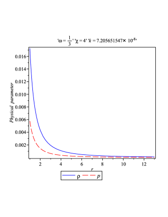
Figure 1: Variations of density $\rho$ ($km^{-2}$) and pressure $p$ ($km^{-2}$) is shown with respect to the radial coordinate $r$ ($km$)

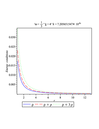
Figure 2: Variations of $\rho$ ($km^{-2}$), $\rho+p$ ($km^{-2}$), and $\rho+3p$ ($km^{-2}$) are shown with respect to the radial coordinate $r$ ($km$)

6.2 TOV equation

From the equation for the non-conservation of the energy-momentum tensor in $f(R,\mathcal{T})$ theory (6) one can obtain the generalized Tolman-Oppenheimer-Volkoff (TOV) equation Moraes2015 for an isotropic fluid distribution (i.e. $p_{r}=p_{t}=p$) as

$$-\frac{\nu^{\prime}}{2}(\rho+p)-\frac{dp}{dr}+\frac{\chi}{8\pi+2\chi}(p^{\prime}-\rho^{\prime})=0,$$ (31)

If one puts $\chi=0$ then one can get the usual form of TOV equation in the case of general relativity. The above TOV equation describes the equilibrium of the stellar configuration under the joint action of three forces, viz. the gravitational force ($F_{g}$), the hydrostatic force ($F_{h}$), and the additional force ($F_{\varkappa}$) due to the modification of the gravitational Lagrangian of the standard Einstein-Hilbert action. So for equilibrium condition one can eventually write it in the following form:

$$F_{g}+F_{h}+F_{\varkappa}=0,$$ (32)

where

$$F_{g}=-\frac{\nu^{\prime}}{2}(\rho+p),$$

$$F_{h}=-\frac{dp}{dr},$$

$$F_{\varkappa}=\frac{\chi}{8\pi+2\chi}(p^{\prime}-\rho^{\prime})$$

.

In the present conformally symmetric model of an isotropic fluid distribution with the EOS $p=\omega\rho$ the TOV equation (31) can be written as

$$-\frac{\nu^{\prime}}{2}(\rho+p)-\frac{dp}{dr}+\frac{\chi}{8\pi+2\chi}(\omega-1)\rho^{\prime}=0.$$ (33)

From Fig. 3 we notice that the static equilibrium has been attained under the mutual action of the three forces $F_{g}$, $F_{h}$ and $F_{\varkappa}$. Also it is observed from the figure that $F_{g}$ and $F_{\varkappa}$ are essentially of the same nature - quantitatively as well as qualitatively.

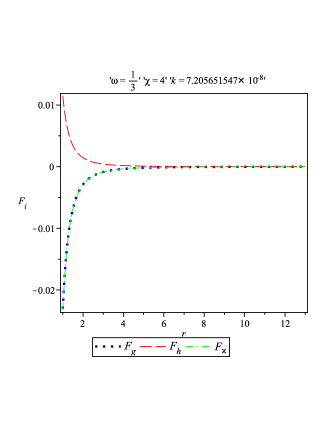
Figure 3: The three different forces, viz. the gravitational force $(F_{g})$, the hydrostatic force $(F_{h})$, and the additional force $(F_{\varkappa})$ are plotted against $r$ ($km$)

6.3 Stability

6.3.1 Sound Speed

According to Herrera herrera1992 for a physically acceptable model the square of the sound speed, i.e. $v_{s}^{2}=\frac{dp}{d\rho}$, within the matter distribution should be in the limit [0,1]. In our model of an isotropic matter distribution we see that $v_{s}^{2}=\frac{dp}{d\rho}=\omega=1/3~{}<1$. Hence our model maintains stability.

6.3.2 Adiabatic Index

The dynamical stability of the stellar model against an infinitesimal radial adiabatic perturbation, which was introduced by Chandrasekhar chandrasekhar1964 , has also been tested in our model. This stability condition was developed and used at astrophysical level by several authors bardeen1966 ; knutsen ; mak2013 .

The adiabatic index is defined by

$$\gamma=\left(\frac{\rho+p}{p}\right)\left(\frac{dp}{d\rho}\right).$$ (34)

For stable configuration $\gamma$ should be $>\frac{4}{3}$ within the isotropic stellar system. However, we have analytically calculated the value of the adiabatic index as $\gamma=\frac{4}{3}$ which is the critical value of $\frac{4}{3}$ chandrasekhar1964 ; Bondi1964 ; Wald1984 .

6.4 Mass-Radius relation

The mass function within the radius $r$ is given by

$$M(r)=\int_{0}^{r}4\pi r^{\prime 2}\rho dr^{\prime}=\frac{4\pi}{\alpha}\left[-\frac{3kr^{(-\beta+1)}}{(-\beta+1)}-\frac{3\sigma r}{\beta}+r\right].$$ (35)

The profile of the mass function has been depicted in Fig. 4, which clearly shows that, for $r\rightarrow 0$, $M(r)\rightarrow 0$, implying the regularity of the mass function at the center.

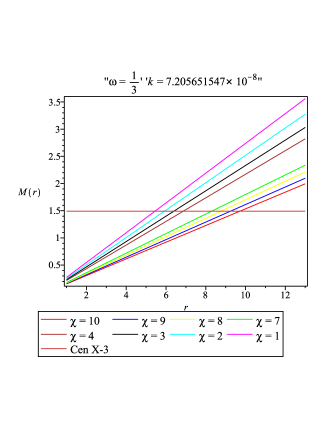
Figure 4: Profile of the mass function $M(r)$ ($km$) is shown with respect to the radial coordinate $r$ ($km$)

According to Buchdahl buchdahl1959 , in the case of a static spherically symmetric perfect fluid distribution the mass to radius ratio $(\frac{2M}{r})$ should be $\leq\frac{8}{9}$. Also Mak et al. mak2001 derived a more simplified expression for the same ratio. In our present model, one can check that Buchdahl’s condition is satisfied (see Fig. 4).

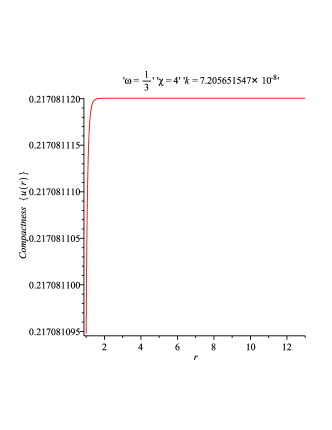
Figure 5: Compactness $u(r)$ is plotted with respect to the radial coordinate $r$ ($km$)

6.5 Compactness and redshift

The compactness of the star $u(r)$ is defined by

$$u(r)=\frac{M(r)}{r}=\frac{4\pi}{\alpha}\left[-\frac{3kr^{-\beta}}{(-\beta+1)}-\frac{3\sigma}{\beta}+1\right].$$ (36)

The profile of the compactness of the star is depicted in Fig. 5.

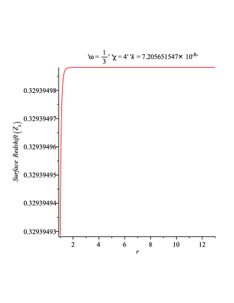
Figure 6: Surface redshift ($Z_{s}$) is plotted with respect to the radial coordinate $r$ ($km$)

The redshift function $Z_{s}$ is defined by

$$Z_{s}=(1-2u)^{-\frac{1}{2}}-1=\left[1-\frac{8\pi}{\alpha}\left(-\frac{3kr^{-\beta}}{(-\beta+1)}-\frac{3\sigma}{\beta}+1\right)\right]^{-\frac{1}{2}}-1.$$ (37)

The profile of the redshift function of the star is depicted in Fig. 6.

7 A comparative study for physical validity of the model

Based on the model under investigation let us carry out a comparative study between the data of the model parameters with that of the compact star candidates. This will provide the status of the presented model as to whether it is valid for observed data set within the allowed constraint. As we do not get the radius of the star theoretically by putting $p=0$ at some radius, therefore, all plots are drawn up to a highest calibrating point of radius 13 km along the $r$-axis, which is sufficient to get information as regards the nature of the compact star.

We have prepared Table 1 where the symbols are used as follows: $D$ = observed radius, $M_{obs}$ = observed mass and $M_{pre}$ = predicted mass. Here in calculation of $M_{pre}$ we have exploited the observed radius $D$, the predicted radius being unable to be determined in the present model as mentioned in the previous paragraph. It is to note that we have drawn all figures assuming $\chi=4$ only except the Fig. 4 for all $\chi$.

Table 1: Comparative study of the physical parameters for compact star and presented model for $\omega=1/3$ and different values of $\chi$ and $k$.

Compact	$M_{obs}$	$D$	$\chi$	$k$	$M_{pre}$	$\frac{M_{obs}}{D}$	$\frac{M_{pre}}{D}$	$Z_{s}(obs)$	$Z_{s}(pre)$
Stars	(in $M_{\odot}$)	(in km)			(in $M_{\odot}$)
$4U1608-52$	1.74 $\pm$ 0.14guver2010a	9.3 $\pm$ 1.0guver2010a	1	$1.594868593\times 10^{-6}$	1.73	0.275968	0.273849	0.493929	0.486914
$VelaX-1$	1.77 $\pm$ 0.08dey2013	9.56 $\pm$ 0.08dey2013	1	$1.594868593\times 10^{-6}$	1.78	0.273091	0.274059	0.484428	0.487604
$4U1820-30$	1.58 $\pm$ 0.06guver2010b	9.1 $\pm$ 0.4guver2010b	2	$5.645562058\times 10^{-7}$	1.55	0.256099	0.251890	0.431786	0.419590
$PSRJ1903+327$	1.667 $\pm$ 0.021dey2013	9.438 $\pm$ 0.03dey2013	2	$5.645562058\times 10^{-7}$	1.612	0.260521	0.251897	0.444945	0.419610
$CenX-3$	1.49 $\pm$ 0.08dey2013	9.178 $\pm$ 0.13dey2013	3	$2.011363054\times 10^{-7}$	1.45	0.239464	0.233199	0.385323	0.368962
$SMCX-4$	1.29 $\pm$ 0.05dey2013	8.831 $\pm$ 0.09dey2013	4	$7.205651547\times 10^{-8}$	1.30	0.215468	0.217076	0.325621	0.329383
$PSRJ1614-2230$	1.97 $\pm$ 0.04 Demorest2010	13 $\pm$ 2 Demorest2010	4	$7.205651547\times 10^{-8}$	1.91	0.223523	0.217085	0.344793	0.329404
$LMCX-4$	1.04 $\pm$ 0.09 dey2013	8.301 $\pm$ 0.2dey2013	7	$3.401707891\times 10^{-9}$	1.01	0.184797	0.179810	0.259476	0.249629
$EXO1785-248$	1.3 $\pm$ 0.2ozel2009	11 $\pm$ 1ozel2009	7	$3.401707891\times 10^{-9}$	1.34	0.174318	0.179809	0.239048	0.249627
$SAXJ1808.4-3658$	0.9 $\pm$ 0.3dey2013	7.951 $\pm$ 1.0dey2013	8	$1.238240496\times 10^{-9}$	0.92	0.166960	0.170079	0.225284	0.231062
$4U1538-52$	0.87 $\pm$ 0.07dey2013	7.866 $\pm$ 0.21dey2013	9	$4.520512257\times 10^{-10}$	0.86	0.163145	0.161340	0.218326	0.215075
$HerX-1$	0.85 $\pm$ 0.15dey2013	8.1 $\pm$ 0.41dey2013	10	$1.654692258\times 10^{-10}$	0.84	0.154790	0.153457	0.203492	0.201175

Note that from the proposed model for $\chi=1-10$ (excluding 5 and 6 which do not provide physically interesting results) we have found out the masses of the compact stars which, in general, are closely equal to the observed values of most of the stars. However, for some values of $\chi$ the model data seems not to provide much significant results for some of the compact stars. It is also interesting to note that in Fig. 4 we have the curve for $\chi=3$ and the straight line parallel to the $r$-axis for $Cen~{}X-3$ total mass. So, the intersection of the two gives the radius as a representaive one. However, the other curves for other values of $\chi$ have no relation with the straight line parallel to the $r$-axis. We also observe from Table 1 that for different $\chi$ all the predicted values of Buchdahl’s ratios fall within the range of observed values of the Buchdahl ratios ($2M/R\leq 8/9\sim 0.88$). On the other hand, the observed and predicted values of the redshift are also very promising as is evident from Table 1 for all the low mass compact stars under investigations.

8 Discussions and conclusions

As discussed in the introductory section, it is argued by Böhmer et al. Boehmer2011 that the $f(T)$ theory of gravity with torsion scalar is more controllable than $f(R)$ theory of gravity with Ricci scalar because the field equations in the former turn out to be the differential equations of second order, whereas in the latter the field equations are in the form of differential equations of fourth order and thus are difficult to handle. On the other hand, the present work on $f(R,\mathcal{T})$ harko2011 is based on another extension of general relativity, which is associated to Ricci scalar $R$ and the trace of the energy-momentum tensor $\mathcal{T}$.

At this juncture one may be curious to perform a comparison between the results of our previous work Das2015 on $f(T)$ gravity and the present work with $f(R,\mathcal{T})$ gravity. However, we are at present very interested to present the model behaviour of compact stars under the $f(R,\mathcal{T})$ theory of gravity assuming the existence of CKV. In connection to the features and hence validity of the model we have explored several physical aspects based on our findings and all these have been reflected to be very interesting advocacy in favor of physically acceptance of the model. Let us now summarize some of these important results as follows:

(i) Density and Pressure: In the present investigation the pressure $p$ and the density $\rho$ blow up as $r\rightarrow 0$ (Fig. 1). This clearly indicates that the core of the star is highly compact and our model is valid for outside of the core. We are unable to estimate the surface density as we do not find any cut on the $r$-axis (i.e. the radius of the star) in the profile of the pressure.

(ii) Energy conditions: In our study we have found through graphical representation that all the energy conditions, namely NEC, WEC, SEC are satisfied within the prescribed isotropic fluid distribution consisting normal matter (Fig. 2).

(iii) TOV equation: The plot for the generalized TOV equation reveals that static equilibrium has been attained by three different forces viz. the gravitational force ($F_{g}$), the hydrostatic force ($F_{h}$), and the additional force ($F_{\varkappa}$) (Fig. 3).

(iv) Stability of the model: Following Herrera herrera1992 it has been observed that the squares of the sound speed remains within the limit [0,1] admitting the condition of causality and hence our model is potentially stable.

We have also studied dynamical stability of the stellar model against the infinitesimal radial adiabatic perturbation where the adiabatic index $\gamma$ has been calculated analytically as $\frac{4}{3}$, which is the critical value for stable configuration chandrasekhar1964 ; Bondi1964 ; Wald1984 .

(v) Buchdahl condition: The mass function within the radius $r$ has been plotted in Fig. 4, which shows that, for $r\rightarrow 0$, $M(r)\rightarrow 0$ implying the regularity of the mass function at the center.

According to Buchdahl buchdahl1959 , in the case of a static spherically symmetric perfect fluid distribution the mass to radius ratio $(\frac{2M}{r})$ should be $\leq\frac{8}{9}$. In the present model, we note that Buchdahl’s condition is satisfied.

(vi) Compactness and redshift: The profile of the compactness of the star has been drawn in Fig. 5 whereas the redshift function $Z_{s}$ of the star has been depicted in Fig. 6. The features as revealed from these figures are physically reasonable.

As one of the major concluding remarks we would like to highlight one special observation that in the present model the profile of the density and the pressure (Fig. 1) reveals that both the density and the pressure suffer from central singularity. Therefore we are unable to make any exact comment on the core of the star, though Figs. 1 and 5 also indicate a high compactness of the core. On the other hand, according to the profile of the mass function (Fig. 4) it maintains the regularity at the center.

Another interesting point can be observed from the assumed data for $\omega=1/3$ which represents an equation of state (EOS) for radiation. However, in the present investigation we have tried to explore other values of the EOS parameter $\omega$ but those do not work well. This seems to indicate that our model suits better for radiating compact stars. In favour of this unique result one can go through some supporting literature Demorest2010 ; LA2001 ; SM2001 ; Govender2003 ; SH2006 ; ARR2016 . But this also immediately raises the problem of the energy conservation in the model. As is well known, in the $f(R,\mathcal{T})$ gravity theory the energy-momentum tensor is not conserved [see Eq. (3)]. This means we may have two probable alternatives: (i) either we must fully investigate and present the energy “conservation” equations for the present model and discuss their possible interpretation as describing radiation emission from the star, (ii) otherwise by maintaining the problem of conservation we have to give up the claim for radiating compact stars in our study assuming that the case for $\omega=1/3$ is just a coincidence out of other several choices of $\omega$ . These intriguing issues may be taken into consideration in a future project.

References

- (1) A.G. Riess et al., Astron. J. 116, 1009 (1998)
- (2) S. Perlmutter et al., Astrophys. J. 517, 565 (1999)
- (3) P. de Bernardis et al., Nature 404, 955 (2000)
- (4) S. Hanany et al., Astrophys. J. 545, L5 (2000)
- (5) P.J.E. Peebles, B. Ratra, Rev. Mod. Phys. 75, 559 (2003)
- (6) T. Padmanabhan, Phys. Repts. 380, 235 (2003)
- (7) T. Clifton, P.G. Ferreira, A. Padilla, C. Skordis, Phys. Rep. 513, 1 (2012)
- (8) J.C. Hwang, H. Noh, Phys. Lett. B 506, 13 (2001)
- (9) N.A. Bahcall et al., Nature 284, 1481 (1999)
- (10) M. Demianski et al., Astron. Astrophys. 454, 55 (2006)
- (11) V. Singh, C.P. Singh, Astrophys. Space Sci. 356, 153 (2015)
- (12) C.G. Böhmer, A. Mussa, N. Tamanini, Class. Quantum Gravit. 28, 245020 (2011)
- (13) P. Wu, H.W. Yu, Phys. Lett. B 692, 176 (2010)
- (14) P.Y. Tsyba, I.I. Kulnazarov, K.K. Yerzhanov, R. Myrzakulov, Int. J. Theor. Phys. 50, 1876 (2011)
- (15) J.B. Dent, S. Dutta, E.N. Saridakis, JCAP 1101, 009 (2011)
- (16) S.H. Chen, J.B. Dent, S. Dutta, E.N. Saridakis, Phys. Rev. D 83, 023508 (2011)
- (17) G.R. Bengochea, Phys. Lett. B 695, 405 (2011)
- (18) P. Wu, H.W. Yu, Phys. Lett. B 693, 415 (2010)
- (19) R.J. Yang, Europhys. Lett. 93, 60001 (2011)
- (20) Y. Zhang, H. Li, Y. Gong, Z.H. Zhu, JCAP 1107, 015 (2011)
- (21) B. Li, T.P. Sotiriou, J.D. Barrow, Phys. Rev. D 83, 064035 (2011)
- (22) P. Wu, H.W. Yu, Eur. Phys. J. C 71, 1552 (2011)
- (23) K. Bamba, C.Q. Geng, C.C. Lee, L.W. Luo, JCAP 1101, 021 (2011)
- (24) M. Krššák, E.N. Saridakis, Class. Quantum Gravit. 33, 115009 (2016)
- (25) S.B. Nassur, C. Ainamon, M.J.S. Houndjo, J. Tossa (2016). arXiv:1602.03172 [gr-qc]
- (26) S.B. Nassur, M.J.S. Houndjo, I.G. Salako, J. Tossa (2016). arXiv:1601.04538 [physics.gen-ph]
- (27) Yi-Fu Cai, S. Capozziello, M. De Laurentis, E.N. Saridakis, Rept. Prog. Phys. 79, 106901 (2016)
- (28) K. Bamba, S.D. Odintsov, E.N. Saridakis (2016). arXiv:1605.02461 [gr-qc]
- (29) C. Deliduman, B. Yapiskan (2011). arXiv:1103.2225 [gr-qc]
- (30) T. Wang, Phys. Rev. D 84, 024042 (2011)
- (31) M.H. Daouda, M.E. Rodrigues, M.J.S. Houndjo, Eur. Phys. J. C 71, 1817 (2011)
- (32) G. Abbas, A. Kanwal, M. Zubair, Astrophys. Space Sci. 357, 109 (2015)
- (33) G. Abbas, S. Qaisar, A. Jawad, Astrophys. Space Sci. 359, 57 (2015)
- (34) A. Das, F. Rahaman, B.K. Guha, S. Ray, Astrophys. Space Sci. 358, 36 (2015)
- (35) S. M. Carroll, V. Duvvuri, M. Trodden, M. S. Turner, Phys. Rev. D 70, 043528 (2004)
- (36) S. Capozziello, S. Nojiri, S.D. Odintsov, A. Troisi, Phys. Lett. B 639, 135 (2006)
- (37) S. Nojiri, S.D.Odintsov, Phys. Rev. D 74, 086005 (2006)
- (38) S. Nojiri, S.D. Odintsov, Phys. Rept. 505, 59 (2011)
- (39) T.P. Sotiriou, V. Faraoni, Rev. Mod. Phys. 82, 451 (2010)
- (40) F.S.N. Lobo, Dark Energy - Current Advances and Ideas. Research Signpost, p. 173, ISBN 978-81-308-0341-8 (2009)
- (41) S. Capozziello, V. Faraoni, Beyond Einstein Gravity (Springer, Netherlands, 2010)
- (42) S. Capozziello, M. De Laurentis, Phys. Repts. 509, 167 (2011)
- (43) T. Harko, F.S.N. Lobo, S. Nojiri, S.D. Odintsov, Phys. Rev. D 84, 024020 (2011)
- (44) P.H.R.S. Moraes, Astrophys. Space Sci. 352, 273 (2014)
- (45) P.H.R.S. Moraes, Eur. Phys. J. C 75, 168 (2015)
- (46) P.H.R.S. Moraes, Int. J. Theor. Phys. 55, 1307 (2016)
- (47) C.P. Singh, P. Kumar, Eur. Phys. J. C 74, 11 (2014)
- (48) P. Rudra, Eur. Phys. J. Plus 130, 9 (2015)
- (49) E.H. Baffou, A.V. Kpadonou, M.E. Rodrigues, M.J.S. Houndjo, J. Tossa, Astrophys. Space Sci. 356, 173 (2015)
- (50) H. Shabani, M. Farhoudi, Phys. Rev. D 88, 044048 (2013)
- (51) H. Shabani, M. Farhoudi, Phys. Rev. D 90, 044031 (2014)
- (52) M. Sharif, M. Zubair, Astrophys. Space Sci. 349, 457 (2014)
- (53) S. Ram, Priyanka, Astrophys. Space Sci. 347, 389 (2013).doi: 10.1007/s10509-013-1517-z
- (54) D.R.K. Reddy, R.S. Kumar, Astrophys. Space Sci. 344, 253 (2013)
- (55) P. Kumar, C.P. Singh, Astrophys. Space Sci. 357, 120 (2015)
- (56) M.F. Shamir, Eur. Phys. J. C 75, 354 (2015)
- (57) V. Fayaz, H. Hossienkhani, Z. Zarei, N. Azimi, Eur. Phys. J. Plus 131, 22 (2016)
- (58) M. Sharif, Z. Yousaf, Astrophys. Space Sci. 354, 471 (2014)
- (59) I. Noureen, M. Zubair, Astrophys. Space Sci. 356, 103 (2015)
- (60) I. Noureen, M. Zubair, Eur. Phys. J. C 75, 62 (2015)
- (61) I. Noureen et al., Eur. Phys. J. C 75, 323 (2015)
- (62) M. Zubair and I. Noureen, Eur. Phys. J. C 75, 265 (2015)
- (63) M. Zubair, G. Abbas, Ifra Noureen, Astrophys. Space Sci. 361, 8 (2016)
- (64) A. Alhamzawi, R. Alhamzawi, Int. J. Mod. Phys. D 25, 1650020 (2015)
- (65) P.H.R.S. Moraes, J.D.V. Arbañil, M. Malheiro, JCAP 06, 005 (2016)
- (66) S. Ray, A.A. Usmani, F. Rahaman, M. Kalam, K. Chakraborty, Ind. J. Phys. 82, 1191 (2008)
- (67) F. Rahaman, M. Jamil, R. Sharma, K. Chakraborty, Astrophys. Space Sci. 330, 249 (2010)
- (68) F. Rahaman, M. Jamil, M. Kalam, K. Chakraborty, A. Ghosh, Astrophys. Space Sci. 137, 325 (2010)
- (69) A.A. Usmani, F. Rahaman, S. Ray, K.K. Nandi, P.K.F. Kuhfittig, Sk.A. Rakib, Z. Hasan, Phys. Lett. B 701, 388 (2011)
- (70) P. Bhar, Astrophys. Space Sci. 354, 457 (2014)
- (71) F. Rahaman et al., Int. J. Mod. Phys. D 23, 1450042 (2014)
- (72) F. Rahaman, S. Ray, G.S. Khadekar, P.K.F. Kuhfittig, I. Karar, Int. J. Theor. Phys. 54, 699 (2015)
- (73) F. Rahaman, A. Pradhan, N. Ahmed, S. Ray, B. Saha, M. Rahaman, Int. J. Mod. Phys. D 24, 1550049 (2015)
- (74) L. Herrera, , J. Jimenez, L. Leal, J. Ponce de Leon,M. Esculpi, V. Galina, J. Math. Phys. 25, 3274 (1984)
- (75) L. Herrera, J. Ponce de Leon, J. Math. Phys. 26, 778 (1985)
- (76) L. Herrera, J. Ponce de Leon, J. Math. Phys. 26, 2018 (1985)
- (77) L. Herrera, J. Ponce de Leon, J. Math. Phys. 26, 2302 (1985)
- (78) M.K. Mak, T. Harko, Int. J. Mod. Phys. D 13, 149 (2004)
- (79) O.J. Barrientos, G.F. Rubilar, Phys. Rev. D 90, 028501 (2014)
- (80) C.G. Böhmer, T. Harko, F.S.N. Lobo, Phys. Rev. D 76, 084014 (2007)
- (81) Böhmer, C.G., Harko, T., Lobo, F.S.N., Class. Quantum Gravit. 25, 075016 (2008)
- (82) L. Herrera, Phys Lett. A 165, 206 (1992)
- (83) S. Chandrasekhar, Astrophys J. 140, 417 (1964)
- (84) J.M. Bardeen, K.S. Thorne, D.W. Meltzer, Astrophys J. 145, 505 (1966)
- (85) H. Knutsen, MNRAS 232, 163 (1988)
- (86) M.K. Mak, T. Harko, Eur Phys. J. C 73, 2585 (2013)
- (87) H. Bondi, Proc. R. Soc. Lond. Series A, Math. Phys.Sci. 281, 39 (1964)
- (88) R.M. Wald, General Relativity (Chicago Press, Chicago and London, 1984), p. 127
- (89) H.A. Buchdahl, Phys. Rev. 116, 1027 (1959)
- (90) M.K. Mak, P.N. Dobson, T. Harko , Europhys. Lett. 55, 310 (2001)
- (91) T. Güver, P. Wroblewski , L. Camarota, F. Özel, Astrophys J. 719, 1807 (2010)
- (92) T. Gangopadhyay, S. Ray, X.-D. Li, J. Dey, M. Dey, Mon. Not. R. Astron. Soc. 431, 3216 (2013)
- (93) T. Güver, P. Wroblewski , L. Camarota, F. Özel, Astrophys J. 712, 964 (2010)
- (94) P.B. Demorest, T. Pennucci, S.M. Ransom, M.S.E. Roberts, J.W.T. Hessels, Nature 467, 1081 (2010)
- (95) F. Özel, T. Güver, D. Psaltis, Astrophys J. 693, 1775 (2009)
- (96) F.C. Lázaro, M.J. Arévalo, Binary stars: selected topics on observations and physical processes, EADN School XII (Springer, Heidelberg, 2001), p. 295
- (97) R. Sharma, S. Mukherjee S, Mod. Phys. Lett. A 16, 1049 (2001)
- (98) M. Govender, K.S. Govinder, S.D. Maharaj, R. Sharma, S. Mukherjee, T.K. Dey, Int. J. Mod. Phys. D 12, 667 (2003)
- (99) D.M. Sedrakian, M.V. Hayrapetyan, Volume 197 of the series NATO Science Series II: Mathematics, Physics and Chemistry, Superdense QCD Matter and Compact Stars (Springer, Netherlands, 2006), pp.43-51
- (100) A. Aziz, S. Ray, F. Rahaman, Eur. Phys. J. C 76, 248 (2016)