A new look on the stabilization of inverted pendulum with parametric excitation and large random frequencies: analytical and numerical approaches

Abstract

In this paper we explore the stability of an inverted pendulum with generalized parametric excitation described by a superposition of $N$ sines with different frequencies and phases. We show that when the amplitude is scaled with the frequency we obtain the stabilization of the real inverted pendulum, i.e., with values of $g$ according to planet Earth ($g\approx 9.8$ m/s²) for high frequencies. By randomly sorting the frequencies, we obtain a critical amplitude in light of perturbative theory in classical mechanics which is numerically tested by exploring its validity regime in many alternatives. We also analyse the effects when different values of $N$ as well as the pendulum size $l$ are taken into account.

1 Introduction

The inverted pendulum and its stability are subjects widely explored in Physics, Engineering, Biology [1], and many other areas due to its technological importance. An inverted pendulum is unstable unless some kind of excitation/vibration is applied to its suspension point (its basis). Kaptiza [2, 3] observed that an inverted pendulum should be stabilized by rapidly oscillating its basis. The limit of stability considering a periodic function at the basis of pendulum has been studied by many authors (see for example [4, 5, 6]). In another context, chaos and bifurcations have been studied for a sinusoidal excitation where both excitation frequencies and amplitudes were varied [7]. However, this excitation can be more general openning a long way to explore the stochastic aspects in the stabilization.

By denoting $z(t)$ as a vertical excitation, the Lagrangian of a pendulum with mass $m$ can be written as

$$\begin{array}[]{lll}\mathcal{L}(\theta,\dot{\theta},z,\dot{z})&=&\frac{1}{2}ml^{2}\left(\dot{\theta}^{2}+\frac{1}{l^{2}}\dot{z}^{2}(t)\right)-ml\dot{z}(t)\dot{\theta}\sin\theta\\ &&-mgz(t)-mgl\cos\theta\end{array}$$ (1)

where the axis $z$ is oriented up, $\vec{a}=-g\hat{z}$ is the gravitational acceleration, and $l$ is the pendulum length, which in turn, leads to the following equation of motion

$$\frac{d^{2}\theta}{dt^{2}}=\frac{g}{l}\left(1+\frac{1}{g}\ddot{z}\right)\sin\theta.$$ (2)

Assuming $\overset{..}{z}$ as a generic time-dependent function and taking into account the limit of small oscillations $\sin\theta\approx\theta$, one has

$$\ddot{\theta}=\left(\omega_{0}^{2}+\frac{1}{l}\ddot{z}\right)\theta,$$ (3)

where $\omega_{0}^{2}=g/l$.

An interesting choice is to consider a parametric excitation

$$z(t)=\sum_{i=1}^{N}A_{i}\sin(\omega_{i}t+\varphi_{i}),$$ (4)

where $A_{i}$, $\omega_{i}$, and $\varphi_{i}$ are arbitrary amplitudes, frequencies and phases, respectively, and $i=1,...,N$. A detailed study of this kind of excitation in an inverted pendulum can be found, for example, in Refs. [1, 8]. In a very different context, Dettmann et al. [9] had obtained an equation for the distance between two photons that propagate in a universe of negative curvature. This distance can be written as

$$\ddot{\theta}=\left(1-f(t)\right)\theta.$$ (5)

At a first glance, this result seems to be a particular case of Eq. (3), where $\omega_{0}^{2}=1$ and $f(t)$ is a stochastic forcing function that, in their particular case, takes into account the perturbation in the curvature due to mass distribution $\omega_{0}^{2}=1$. They studied the stochastic stabilization of Eq. (5) by considering

$$f(t)=f_{D}(t)=A\sum_{i=1}^{N}\sin(\omega_{i}t+\varphi_{i}),$$ (6)

where $A$ is a control parameter and $\left\{\omega_{i},\varphi_{i}\right\}_{i=1}^{N}$ are chosen independently at random according to a uniform distribution defined on supports: $[\omega_{\min},\omega_{\max}]$ and $[\phi_{\min},\phi_{\max}]$ respectively.

It is important to emphasize that by simply making $\omega_{0}^{2}=1$ in Eq. (3) with $A_{i}=A$ in Eq. (4), we do not recover Eq. (5), since the usual $f(t)$ considered for a regular pendulum is

$$f(t)=f_{S}(t)=-\frac{1}{l}\overset{..}{z}(t)=\frac{1}{l}\sum_{i=1}^{N}A_{i}\omega_{i}^{2}\sin(\omega_{i}t+\varphi_{i}).$$ (7)

At this point two technical problems occur. Firstly, $\omega_{0}^{2}=1$ means the specific case of a huge pendulum ($l\approx 9.8$ m). Secondly, we should incorporate the gravity $g$ in $A$. However, the term $\omega_{i}^{2}$ does not exist in the original problem considered by Dettman et al. [9].

The main contributions of this paper is related to the stabilization of the inverted pendulum or similar system. Here, we answer the following two questions and compare both situations:

1. Is it possible to stabilize an inverted pendulum in a general situation, i.e., by considering the Eq. (3) with the parametric excitation $z(t)=A\sum_{i=1}^{N}\sin(\omega_{i}t+\varphi_{i})$ with random frequencies uniformily distributed in $[\omega_{\min},\ \omega_{\max}]$? If yes, what should be the parameters $\omega_{0}$ and $A$?

2. Is it possible to obtain a more general stabilization criteria by considering any values of parameters $\omega_{\min},\ \omega_{\max}$ and $A$? This question arises because Dettman et al. showed that the problem for a particular cosmological application (Eqs. (5) and (6)) can be “stochastically” stabilized when considering a specific choice of $\omega_{\min},\ \omega_{\max}$ and $A$.

Throughout this work we will present the answer of these questions. However, we would like to point out that the answer is yes, we are able to stabilize the inverted pendulum by considering more general criterias.

Our manuscript is organized as follows: In the next section, we present the perturbative calculations in detail and show a general solution for the problem. For this purpose, we consider the more general equation

$$\ddot{\theta}=\left(\omega_{0}^{2}-f(t)\right)\theta$$ (8)

with a more general function

$$f(t)=\sum_{i=1}^{N}A_{i}^{\ast}\sin(\omega_{i}t+\varphi_{i})$$

where $\omega_{0}^{2}=1$ and $A_{i}^{\ast}=A$ correspond to the cosmological problem (Problem I) and $\omega_{0}^{2}=\frac{g}{l}$ and $A_{i}^{\ast}=\frac{\omega_{i}^{2}}{l}A_{i}$, $i=1,2,...,N$ correspond to the general regular inverted pendulum (Problem II). In Sec. 3 we show our results and the conclusions are presented in Sec. 3.

2 Perturbative methods

In this section we describe in detail how to obtain a general stability condition to the Eq. (8). An interesting Ansatz to start with is:

$$\theta(t)=\phi_{slow}(t)+\omega^{-\alpha}\phi_{fast}(t)$$ (9)

where the motion in decomposed in two parts: one slow and another fast. The fast part corresponds to an additional noise to the main motion (the slow one). The ad hoc parameter $\omega^{-\alpha}$ controls the contribution of the fast component, and $\alpha$ is a positive number which characterizes this term. The quantity $\omega=2\pi/T$ is an average over the differents $\{\omega_{i}\}_{i=1}^{N}$.

By substituting Eq. (9) into Eq. (8) we obtain

$$\begin{array}[]{lll}\overset{\cdot\cdot}{\phi}_{slow}(t)+\omega^{-\alpha}\overset{\cdot\cdot}{\phi}_{fast}(t)&=&\omega_{0}^{2}\phi_{slow}(t)-f(t)\phi_{slow}(t)\\ &&+\omega^{-\alpha}\omega_{0}^{2}\phi_{fast}(t)\\ &&-\omega^{-\alpha}f(t)\phi_{fast}(t)\end{array}$$ (10)

Now it is crucial to consider the nature of motion to distinguish the important terms in Eq. (10). The only candidates associated with the perturbative effects on the right side of this equation are $-f(t)\phi_{slow}(t)$, $\omega^{-\alpha}\omega_{0}^{2}\phi_{fast}(t)$, and $\omega^{-\alpha}f(t)\phi_{fast}(t)$. Therefore, given that the terms $\omega^{-\alpha}\omega_{0}^{2}\phi_{fast}(t)$ and $\omega^{-\alpha}f(t)\phi_{fast}(t)$ are small when compared with $-f(t)\phi_{slow}(t)$ we have

$$\omega^{-\alpha}\overset{\cdot\cdot}{\phi}_{fast}(t)\approx-f(t)\phi_{slow}(t).$$ (11)

Let us define the time average as

$$\left\langle g\right\rangle(t)=\mathbf{\ }\int_{-\infty}^{\infty}g(\tau)\Phi_{T}(\tau-t)d\tau$$ (12)

where,

$$\Phi_{T}(\tau-t)=\left\{\begin{array}[]{ccc}1/T&&\text{if }\left|\tau-t\right|<T/2\\ &&\\ 0&&\text{otherwise}\end{array}\right.$$ (13)

where $T$ is small and by hyphotesis/construction $\left\langle\phi_{fast}\right\rangle=0$. Here, $\lim_{T\rightarrow 0}\Phi_{T}(\tau-t)=\delta(\tau-t)$, which corresponds to the limit $\omega\rightarrow\infty$.

In this case one has

$$\left\langle\phi_{slow}(t)\right\rangle\approx\int_{-\infty}^{\infty}\phi_{slow}(\tau)\delta(\tau-t)d\tau=\phi_{slow}(t)$$ (14)

and similarly

$$\left\langle\overset{\cdot\cdot}{\phi}_{slow}(t)\right\rangle\approx\int_{-\infty}^{\infty}\overset{\cdot\cdot}{\phi}_{slow}(\tau)\delta(\tau-t)dt\tau=\ \overset{\cdot\cdot}{\phi}_{slow}(t).$$ (15)

Now, with the choice of a fast oscillatory function $f(t)$ such that $\left\langle f(t)\right\rangle=0$ for some time interval $t$, and $\left\langle\phi_{slow}(t)\right\rangle\approx$ $\phi_{slow}(t)$ in this time range, then it is easy to show that $\left\langle f(t)\phi_{slow}(t)\right\rangle\approx\phi_{slow}(t)\left\langle f(t)\right\rangle\approx 0$. After all these constraints, and taking the time average according to Eq. (10) the dynamics of the slow component can be written as

$$\overset{\cdot\cdot}{\phi}_{slow}(t)=\omega_{0}^{2}\phi_{slow}(t)-\omega^{-\alpha}\left\langle f(t)\phi_{fast}(t)\right\rangle.$$ (16)

By integrating Eq. (11) and having in mind that $\phi_{slow}(t)$ has a slow variation, one has:

$$\omega^{-\alpha}\overset{\cdot}{\phi}_{fast}(t)\approx-\phi_{slow}(t)\int_{0}^{t}f(s)ds$$ (17)

considering that $\overset{\cdot}{\phi}_{fast}(0)=0$. In the same way, by integrating again yields

$$\omega^{-\alpha}\phi_{fast}(t)\approx-\phi_{slow}(t)x(t),$$ (18)

where $x(t)=\int_{0}^{t}v(s)ds$ with $v(t)=\int_{0}^{t}f(s)ds$, and $\phi_{fast}(0)=0$ by hypothesis.

Multiplying the Eq. (18) by $f(t)$ and taking the average again, one has: $\omega^{-\alpha}\left\langle f(t)\phi_{fast}(t)\right\rangle\approx-\phi_{slow}(t)\left\langle f(t)x(t)\right\rangle$. Let us now calculate $\left\langle f(t)x(t)\right\rangle$. According to Eq. (12), this average is given by

$$\left\langle f(t)x(t)\right\rangle=\frac{1}{T}\int_{0}^{T}\frac{dv}{dt}x(t)dt.$$

Integrating the above equation by parts one has

$$\begin{array}[]{lll}\left\langle f(t)x(t)\right\rangle&=&\frac{1}{T}\int_{0}^{T}\frac{dv(t)}{dt}x(t)dt\\ &&\\ &=&\frac{1}{T}\left[v(T)x(T)-v(0)x(0)\right]-\frac{1}{T}\int_{0}^{T}v(t)\frac{dx}{dt}(t)dt\\ &&\\ &=&-\frac{1}{T}\int_{0}^{T}v^{2}(t)dt=-\left\langle v^{2}(t)\right\rangle\end{array}$$

providing $\omega^{-\alpha}\left\langle f(t)\phi_{fast}(t)\right\rangle\approx-\phi_{slow}(t)\left\langle f(t)x(t)\right\rangle=\phi_{slow}(t)\left\langle v^{2}(t)\right\rangle$. The Eq. (16) can then be written as

$$\overset{\cdot\cdot}{\phi}_{slow}(t)=\left[\omega_{0}^{2}-\left\langle v^{2}(t)\right\rangle\right]\phi_{slow}(t).$$ (19)

3 Results

Let us start by considering the problem of a real inverted pendulum, the problem previously called problem II. So, $f(t)=\frac{1}{l}\sum_{i=1}^{N}A_{i}\omega_{i}^{2}\sin(\omega_{i}t+\varphi_{i})$ and $\omega_{0}^{2}=g/l$. In addition, it is convenient to consider $A_{i}=l\frac{A}{\omega_{i}^{2}}$ whereas we are looking for a general and broad treatment for the two problems raised in this work, simultaneously.

This means that if the frequencies are chosen at random according to a uniform probability distribution, the amplitudes must be scaled by dividing them by the square of those frequencies.

Here it is also important to observe that $\left\langle v^{2}(t)\right\rangle$ in Eq.(19) is a time-dependent function, since

$$v(t)=-A\sum_{i=1}^{N}\frac{1}{\omega_{i}}\sin(\omega_{i}t+\varphi_{i})$$

The square of this equation yields $v(t)^{2}=A^{2}\sum_{i=1}^{N}\frac{1}{\omega_{i}^{2}}\sin^{2}(\omega_{i}t+\varphi_{i})+A^{2}\sum_{i\neq j=1}^{N}\frac{1}{\omega_{i}\omega_{j}}\sin(\omega_{i}t+\varphi_{i})\sin(\omega_{j}t+\varphi_{i})$.

However, we can make an ad hoc consideration, which is a kind of “mean-field approximation”, by changing $\left\langle v^{2}(t)\right\rangle$ by a simple time average. This means to consider $\left\langle v^{2}(t)\right\rangle$ as a constant $\overline{v^{2}}$, i.e.,

$$\overline{v^{2}} = A^{2}\sum_{i=1}^{N}\frac{1}{\omega_{i}^{2}}\overline{\sin^{2}(\omega_{i}t+\varphi_{i})}$$

$$+A^{2}\sum_{i\neq j=1}^{N}\frac{1}{\omega_{i}\omega_{j}}\overline{\sin(\omega_{i}t+\varphi_{i})\sin(\omega_{j}t+\varphi_{i})}$$

which leads to

$$\begin{array}[]{lll}\overline{v^{2}}&=&\frac{A^{2}}{2}\sum_{i=1}^{N}\omega_{i}^{-2}\\ &&\\ &\approx&\frac{N}{2(\omega_{\max}-\omega_{\min})}A^{2}\int_{\omega_{\min}}^{\omega_{\max}}\omega^{-2}d\omega\\ &&\\ &=&\frac{N}{2}\frac{A^{2}}{\omega_{\max}\omega_{\min}},\end{array}$$

which, in turn, leads to the stability condition:

$$\omega_{0}^{2}<\frac{N}{2}A^{2}\frac{1}{\omega_{\max}\omega_{\min}}.$$

More simply,

$$A\geq A_{c}(\omega_{\min},\omega_{\max})=\sqrt{\frac{2g}{Nl}\omega_{\max}\omega_{\min}}.$$ (20)

In order to verify our approach, we take into account frequencies chosen at random in the interval $[\omega_{\min},\omega_{\max}]$ and look into the stabilization of the inverted pendulum. Considering these frequencies, our perturbative analysis provides a lower bond for the amplitude $A$ which is tested through numerical simulations.

In our simulations, we numerically integrate the Eq. (8) using the fourth-order Runge-Kutta method [10] with $f(t)=\sum_{i=1}^{N}A\sin(\omega_{i}t+\varphi_{i})$ starting from $\theta_{0}=1^{o}\approx 0.018$ rad and $\dot{\theta}_{0}=0$.

First, we fix the amplitude $A$ and randomly sort $N$ frequencies $\omega_{i}$, $i=1,...,N$ with uniform distribution in the interval $[\omega_{\min},\omega_{\max}]$. In addition, we also sort $N$ random phases $\varphi_{i}$, $i=1,...,N$ in the interval $[-\pi,\pi]$. Then, we repeat the procedure $N_{run}$ times we test how many times the stability is broken considering a maximum number of iterations $\tau_{\max}=10^{5}$.

Finally, we calculate the following quantities:

1. survival probability: It is denoted by $p=\frac{n}{N_{run}}$, where $n\leq N_{run}$ is the number of times such that the time evolution reaches the maximal number of iterations $\tau_{\max}$.

2. survival time: It is the time $\tau\leq\tau_{\max}$, and describes the first time that the condition $\cos\theta<0$ is satisfied, i.e., the pendulum loses its stability (which is an appropriated and robust stability condition as discussed and numerically verified in Ref. [8]).

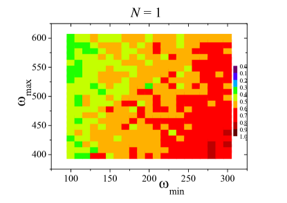
Figure 1: Stability diagrams for $l\overset{N}{=}g=9.8$ m/s² obtained by numerical integration. For each pair ($\omega_{\min},\omega_{\max}$) we draw the survival probability $p$ according to rainbow collor scale (very cold $p\rightarrow 0$ and very hot $p\rightarrow 1$).

In order to perform an exhaustive numerical analysis for each pair ($\omega_{\min},\omega_{\max}$), we build stability diagrams considering the number of sines being added in $f(t)$. Since the results from the perturbative analysis must get better as $N$ increases, it is interesting to study the influence of $N$ on the inverted pendulum stability. We consider the system exactly in $A=A_{c}(\omega_{\min},\omega_{\max})$ (according to Eq. (20)) which is the necessary minimum amplitude according to the perturbative theory previously developed. It is important to notice that our simulations use the critical minimal value $A_{c}$ for the amplitude in order to test the robustness of our theoretical result given by Eq. (20), whereas larger amplitudes should bring more stability. The idea of fixing $A=A_{c}(\omega_{\min},\omega_{\max})$ is interesting because it saves one dimension in the plots that are shown below.

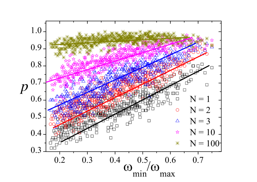
Figure 2: Survival probability ($p$) as function of $\omega_{\min}/\omega_{\max}$ for different number of sines. We can observe that $p$ has a positive correlation with enlarge of $\omega_{\min}$. Here, we also used $l\overset{N}{=}g=9.8$ m/s² and the results were obtained via numerical integration.

Figure 1 shows the survival probability for different minimal/maximal frequency pairs used in this work. After some numerical tests, we adopted $100\leq\omega_{\min}\leq 300$ while $400\leq\omega_{\max}\leq 600$. In order to estimate the survival probability $p$, we used $N_{run}=100$ repetitions. The plots differ in the number $N$ of sines used. According to the adopted rainbow color scale, we can observe that as $N$ enlarges, we have larger $p$. In all the simulations we used $l\overset{N}{=}g=9.8$ $m/s^{2}$.

A plot of $p$ as function of the ratio $\omega_{\min}/\omega_{\max}$ is shown in Fig. 2. We can observe that $p$ has a positive correlation showing that the larger the minimum frequency the more stability is expected.

Following, we test if it is possible to give more flexibility to the stability criteria based previously on fixing the amplitude, according to Eq. (20). In order to proceed this analysis, we calculate the ratio $\left\langle\tau\right\rangle/\tau_{\max}$ considering $A=A_{c}-\varepsilon$ and look into the deviations from stability as the deviation parameter $\varepsilon$ gets larger. Here, $\left\langle\tau\right\rangle$ is survival time averaged by $N_{run}$ repetitions. For that, we consider $\varepsilon=0,2$ and $10$. In order to depict this behavior, a plot of $\left\langle\tau\right\rangle/\tau_{\max}$ as function of the ratio $\omega_{\min}/\omega_{\max}$ is shown in Fig. 3.

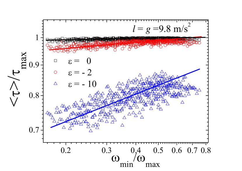
Figure 3: Study of a more flexible stability criteria for the amplitude according to Eq. (20). We can observe that the average of survival time approximates of $\tau_{\max}$ as $\varepsilon\rightarrow 0$. Here, we also used $l\overset{N}{=}g=9.8$ m/s² and $N=100$ and the results were obtained via numerical integration.

It is important to mention that we can observe a positive correlation in the increase of $\left\langle\tau\right\rangle$ when the minimal frequency increases, corroborating the idea that the larger the minimum frequency the more stability is expected.

So far, we have not explored the effects of pendulum size. So, we elaborated similar diagrams presented in Fig. 1, but now changing the pendulum size $l$ in order to study how the stability of the pendulum depends on this parameter.

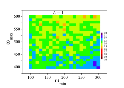
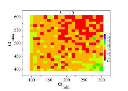
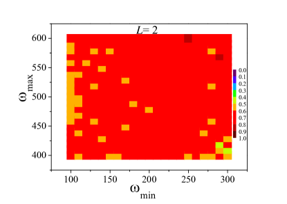
Figure 4: Stability diagrams for different $l$ sizes obtained for numerical integration and keeping $N=100$. For each pair ($\omega_{\min},\omega_{\max}$) we draw the survival probability $p$ according to rainbow color scale (very cold $p\rightarrow 0$ and very hot $p\rightarrow 1$).

We can observe that larger pendulums are most likely stabilized. Table 1 shows the maximum survival probability obtained for all pairs $\left(\omega_{\min},\omega_{\max}\right)$ used in the plots of Fig. 4 for each pendulum size ($l$) studied. In columns 2 and 3 we show the values of $\omega_{\min}$ and $\omega_{\max}$ for which $p_{\max}$ was found. We can observe a systematic increase of $p_{\max}$ as $l$ increases. For $l=9.81$ m, for example, we obtain $p_{\max}=1$.

$l$ (m)	$\omega_{\min}$	$\omega_{\max}$	$p_{\max}$
0.5	180	580	0.24
1.0	200	550	0.34
1.5	190	540	0.50
2.0	250	600	0.64
2.5	250	600	0.72
9.8	230	440	1.00

Table 1: Maximum survival probability for different lengths $l$ of the pendulum

So, we can conclude that the inequality given by Eq. (20) is suitable and therefore can be used in the study of inverted pendulums. This conclusion is supported by numerical simulations which, in addition, describe the effects of $N$ and the size of pendulum on its stability. It is important to notice that deviations of this inequality can be observed for small pendulums but its validity occurs for larger $l$-values.

The next subsection deals with the validity of Eq. (20) for a particular set of parameters and show the range in which the critical amplitude $A_{c}$ is valid.

3.1 Exploring the range of validity of the critical amplitude and scaling

Let us now explore in more detail the validity of the critical amplitude, previously calculated via perturbative analysis, by considering numerical simulations. This study makes possible to better explore the scaling properties of the survival probability ($p$). To perform the simulations, we fixed the frequencies in $\omega_{\min}=300$ and $\omega_{\max}=600$ and set $l\overset{N}{=}g=9.8$ $m/s^{2}$, for which we are sure that $p_{\max}=1$ (see Table 1). We also used the same number of repetitions (as in the previous analysis) to estimate $p$: $N_{run}=100.$ We performed numerical integrations considering several different number of sines, $10\leq N\leq 100$, with $\Delta N=10$, in order to obtain $p$ as function of the amplitude $A$. First, we show in Fig. 5 (a) two curves for $N=10$ and $N=40$ as function of $A$.

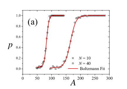
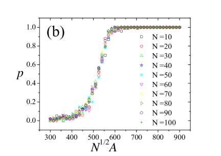
Figure 5: (a) Survival probability $p$ as function of the amplitude $A$ for two different number of sines used in numerical results: $N=10$ and $N=40$. The points correspond to numerical results while the lines correspond to the Boltzmann fits. (b) Collapse of curves $p\times N^{1/2}A$. We can observe that all curves, corresponding to different number of sines, become practically the same universal curve, under scaling $A\rightarrow N^{1/2}A$.

The typical transition from $p=0$ to $p=1$ suggests a familiar fit, known as Boltzmann curve which is parameterized as

$$p=p_{\min}+\frac{(p_{\max}-p_{\min})}{1+\exp\left[\frac{(A-A_{0})}{\Delta}\right].}$$ (21)

Therefore we performed fits according to this function as shown in Fig. 5 (a) by the lines in red which can be compared with the points obtained from our numerical integration. The nonlinear fit, taking into account the Levenberg–Marquardt algorithm (see for example [10]), yields for $N=10$, the parameters $p_{\min}=0.020(7)$, $p_{\max}=1.003(5)$, $A_{0}=165.3(4)$, and $\Delta=9.5(3)$, while for $N=40$, we obtained the parameters $p_{\min}=0.032(6)$, $p_{\max}=1.004(4)$, $A_{0}=82.21(17)$, and $\Delta=4.15(15)$. We also obtained an excelent fit with the coefficient of determination $\alpha=0.998$ in both cases (the closer to 1, the better is the fit).

Another important question here is that the analytical result from Eq. 20 indicate that $A_{c}\sim N^{-1/2}$. This suggests a scaling relation for the survival probability:

$$p(A,N)=h(b^{-1/2}A,bN).$$

By imposing the scaling $bN=1$, we have$p(A,N)=h(N^{1/2}A,1)$ where $h(x,1)=h(x)$ has the property:

$$h(x)=\left\{\begin{array}[]{ccc}1&\text{if}&x\rightarrow\infty\\ &&\\ 0&\text{if}&x\rightarrow 0\end{array}\right.$$

In Fig. 5 (b) we show the curves $p\times N^{1/2}A$ for different values of $N$. We can observe a collapse of all curves through the finite size scaling considered according to our previous description. But what to say about $A_{c}$? Can we obtain the analytical prediction described by Eq. 20 from these numerical results? Yes. Actually the procedure is very simple. We can numerically estimate $A_{c}$ from the plots $p\times A$ by taking the first value of $A$ (the numerical critical amplitude) such that the survival probability is exactly equal to 1. After, we can compare this numerical result with $A_{c}$ obtained analitically through Eq. 20. Figure 6 shows a good agreement between these two analysis which, as can be seen, becomes better for larger values of $N$.

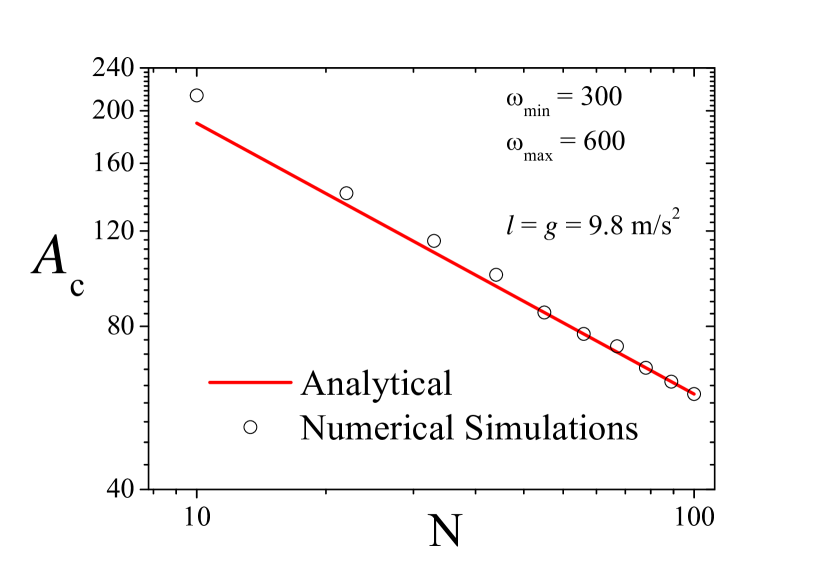
Figure 6: Log-log plot of $A_{c}\times N$. The points correspond to numerical estimates while the line corresponds to analytical estimates. We can see a good agreement between the results which becomes better as $N$ increases.

Thus, our results corroborate the analytical estimate for the critical amplitude obtained from perturbation theory. In addition, the scaling $A\rightarrow N^{1/2}A$ produces a collapse of all survival probabilities. The same procedure can be repeated for smaller pendulums. In this case $p_{\max}$ may be less than 1 and the numerical procedures for determining $A_{c}$ must be more careful.

4 Summary and brief conclusions

By showing an interesting extension of results obtained by Dettman et al. [9] in the context of the stabilization of cosmological photons which are far from parameters of a real pendulum, we fixed $g=9.8$ $m/s^{2}$ and showed that an inverted pendulum can “stochastically” be stabilized under of superposition of sines if the amplitudes are rescaled according to square frequencies.

In our analytical study, we were able to obtain the critical amplitude which depends on the maximum and minimum amplitudes used as parameters to uniformly sort frequencies which were numerically tested considering different number of sines. Our numerical results corroborate the critical lower bound amplitude obtained analytically and, in addition, bring important details about its applicability which cannot be captured by the perturbative analysis. The results show, for example, that as pendulum size increases, more prominent is the verification of the analytical result to the amplitude. We also verify that the number of sines directly impacts on the verification of the lower bound. Moreover, deviations from these theoretical predictions have direct effects in numerical simulations which are observed by tuning a deviation parameter $\varepsilon$ introduced in our analysis. We also conducted an interesting study about finite-size scaling observing the survival probability $p$ as function of the amplitudes $A$. First, we showed that $p\times A$ follows a Boltzmann function moving from $p=0$ ($A<A_{c}$) to $p=1$ ($A>A_{c}$). In addition, our results show that for a large values of $l$, the dependence of $A_{c}$ on $N$, predicted by perturbative analysis, fits very well the numerical results.

It is interesting to say that our analysis does not depend on $\alpha$ that appears in Eq. (9) showing that other dependences can be tested further. It is also important to mention that other distributions of frequencies $\omega$ may be better explored in the future.

Acknowledgments – This research work was in part supported financially by CNPq (National Council for Scientific and Technological Development). R. da Silva would like to thank Prof. L.G. Brunnet (IF-UFRGS) for kindly providing the computational resources from Clustered Computing (cluster-slurm.if.ufrgs.br))

References

References

- [1] R. A. Ibrahim, J. Vib. Control, 12(10), 1093-1170 (2006)
- [2] P. L. Kapitza, Zhur. Eksp. i Teoret. Fiz., 21, 588 (1951)
- [3] P. L. Kapitza, Dynamical stability of a pendulum when its point of suspension vibrates, and Pendulum with a vibrating suspension, in “Collected Papers of P. L.Kapitza”, Ed. by D.ter Haar, Pergamon Press (1965)
- [4] L. D. Landau, E.M. Lifshitz, Mechanics ( Volume 1 of A Course of Theoretical Physics ) Pergamon Press,1969
- [5] E. I. Butikov, Am. J. Phys. 69(6) 1-14 (2001)
- [6] G. Erdos, T. Singh, Journal of Sound and Vibration, 198(5), 643-650 (1996)
- [7] Sang-Yoon Kim and Bambi Hu, Phys. Rev. E 58, 3028 (1998)
- [8] R. da Silva, D. E. Peretti, S. D. Prado, Appl. Math. Model., 40, 10689-10704 (2016).
- [9] C. P. Dettmann, J. P. Keating, S. D. Prado, Int. J. Mod. Phys. D. 13(7) 1-8 (2004)
- [10] W. H. Press, S. A. Teukolsky, W. T. Vetterling, B. P. Flannery, Numerical recipes in Fortran 77: the art of scientific computing, Cambridge University Press, 1992