Sparse image reconstruction on the sphere:
analysis and synthesis

Abstract

We develop techniques to solve ill-posed inverse problems on the sphere by sparse regularisation, exploiting sparsity in both axisymmetric and directional scale-discretised wavelet space. Denoising, inpainting, and deconvolution problems, and combinations thereof, are considered as examples. Inverse problems are solved in both the analysis and synthesis settings, with a number of different sampling schemes. The most effective approach is that with the most restricted solution-space, which depends on the interplay between the adopted sampling scheme, the selection of the analysis/synthesis problem, and any weighting of the $\ell_{1}$ norm appearing in the regularisation problem. More efficient sampling schemes on the sphere improve reconstruction fidelity by restricting the solution-space and also by improving sparsity in wavelet space. We apply the technique to denoise Planck 353 GHz observations, improving the ability to extract the structure of Galactic dust emission, which is important for studying Galactic magnetism.

I Introduction

Spherical images arise in many fields, from cosmology (e.g. [1]) to biomedical imaging (e.g. [2]), where inverse problems are often encountered. Sparse priors have proved highly effective in regularising Euclidean inverse problems, where sparsity is imposed in a wavelet space or sparsifying dictionary. In the spherical setting, wavelet theory is only recently starting to approach maturity, while a mature, general, and robust framework for sparse regularisation is lacking.

Over the last couple of decades there have been many developments regarding wavelet theory in spherical settings. Many initial attempts to extend wavelet transforms to the sphere differed primarily in the manner in which dilations are defined on the sphere [3, 4, 5, 6, 7, 8, 9, 10, 11, 12, 13]. These constructions were essentially based on continuous methodologies, which, although insightful, limited practical application to problems where the exact synthesis of a function from its wavelet coefficients is not required. A number of early discrete constructions followed [14, 15, 16, 17, 18]; however, many of these constructions do not necessarily lead to stable bases [19]. More recently, a number of discrete wavelet frameworks have emerged that have found considerable application, particularly in cosmology (e.g. [20, 21, 22, 23]), including needlets [24, 25, 26]; scale-discretised wavelets [27, 28, 29, 30, 31, 32, 33]; and the isotropic undecimated and pyramidal wavelet transforms [34]. All three of these approaches have also been extended to analyse signals defined on the three- dimensional ball formed by augmenting the sphere with the radial line [35, 36, 37, 38, 39], such as the galaxy distribution.

Solving Euclidean inverse problems by imposing sparse regularising priors has become increasingly popular in recent years. This trend has been driven by improving theoretical foundations for the recovery of sparse signals, facilitated by the theory of compressive sensing [40, 41, 42], and empirical results that have demonstrated the effectiveness of sparse priors for wide classes of natural images. Sparse reconstruction problems can be posed in either the synthesis or analysis settings [43]. In the synthesis setting, the sparse (e.g. wavelet) coefficients of the signal are recovered, from which the signal is synthesised. In the analysis setting, although sparsity is imposed in some sparsifying (e.g. wavelet) dictionary, the signal is recovered directly. When the dictionary considered is not an orthonormal basis but a redundant dictionary, the synthesis and analysis approaches exhibit quite different properties since the solution-space of the analysis problem is more restrictive than the synthesis problem [43, 44, 45]. Empirical studies have shown promising results for the analysis setting (e.g. [43, 46, 47]), which is hypothesised to be due to its more restrictive solution-space.

Some progress has been made towards solving sparse regularisation problems on the sphere (e.g. [48, 49, 50]). Compressive sensing for signals sparse in spherical harmonic space is considered in [49], while inpainting problems are considered in [48, 50], imposing sparsity in a redundant dictionary [48] and the signal gradient [50].

In this work we consider general linear inverse problems on the sphere, including denoising, inpainting, and deconvolution problems, and combinations thereof, and apply sparse regularising priors in scale-discretised wavelet space, using both axisymmetric and directional wavelets [27, 28, 29, 30]. Moreover, for the first time we study in detail the properties and empirical performance of the analysis and synthesis problems on the sphere. Furthermore, we investigate the impact of sampling theorems and schemes on the sphere [51, 52, 53] for sparse image recovery, which have already been shown to play a significant role [50]. In particular, we study the impact of the efficiency of sampling schemes in both the synthesis and analysis settings.

While sparse regularisation is often very effective, we close this introduction by cautioning against the blind application of sparse priors. For example, for the cosmic microwave background (CMB), which is to very good approximation a realisation of a Gaussian random field on the sphere, we recall that inpainting by imposing sparsity in spherical harmonic space (via the $\ell_{1}$ norm) has the undesirable property of breaking statistical isotropy [54]. One must therefore take care in applying priors appropriate for the problem at hand.

The remainder of the article is structured as follows. In Sec. II we review harmonic analysis on the sphere ${\mathbb{S}^{2}}$ and rotation group ${\mathrm{SO}(3)}$ and associated sampling theorems and schemes. In Sec. III we present the general framework to solve inverse problems on the sphere using sparse reconstruction. In Sec. IV we study sparse image reconstruction on the sphere through numerical experiments, comparing the analysis and synthesis settings and evaluating the impact of the sampling scheme used. In Sec. V we apply the methods proposed to denoise the Planck 353 GHz data. In Sec. VI we conclude.

II Sampling on the Sphere and Rotation Group

In this section we review the representation of signals on the sphere and the rotation group, in both the spatial and harmonic domains. We consider discretised signals, sampled according to different sampling schemes and sampling theories, that differ in the number of samples required to capture all of the information content of signals.

II-A Signals on the Sphere

We consider the space of square integrable functions defined on the sphere ${\mathbb{S}^{2}}$. The canonical basis for the space of square integrable functions on the sphere is given by the spherical harmonics $Y_{\ell m}\in\mathrm{L}^{2}({\mathbb{S}^{2}})$, with natural $\ell\in\mathbb{N}$, integer $m\in\mathbb{Z}$ and $|m|\leq\ell$. Due to the orthogonality and completeness of the spherical harmonics, any square integrable function on the sphere $x\in\mathrm{L}^{2}({\mathbb{S}^{2}})$ may be represented by its spherical harmonic expansion

$$x(\omega)=\sum_{\ell=0}^{\infty}\sum_{m=-\ell}^{\ell}{x}_{{\ell}{m}}\>Y_{\ell m}({\omega})\>,$$ (1)

where the spherical harmonic coefficients are given by the usual projection onto each basis function:

$${x}_{{\ell}{m}}=\langle{x},\>{Y_{\ell m}}\rangle=\int_{\mathbb{S}^{2}}\mathrm{\,d}\Omega(\omega)\>x(\omega)\>Y_{\ell m}^{\ast}({\omega})\>,$$ (2)

where $\mathrm{\,d}\Omega(\omega)=\sin\theta\mathrm{\,d}\theta\mathrm{\,d}\varphi$ is the usual invariant measure on the sphere and $\omega=(\theta,\varphi)$ denote spherical coordinates with colatitude $\theta\in[0,\pi]$ and longitude $\varphi\in[0,2\pi)$. Complex conjugation is denoted by the superscript ^∗. Throughout, we consider signals on the sphere band-limited at ${L}$, that is signals such that ${x}_{{\ell}{m}}=0$, $\forall\ell\geq{L}$, in which case the summation over $\ell$ in Eq. (1) may be truncated to the first ${L}$ terms.

In the discrete setting we can write the forward and inverse spherical harmonic transforms as linear operators, respectively:

$$\hat{\mbox{\boldmath${x}$}}=\tilde{\boldsymbol{\mathsf{Y}}}\mbox{\boldmath${x}$},$$ (3)

$$\mbox{\boldmath${x}$}=\boldsymbol{\mathsf{Y}}\hat{\mbox{\boldmath${x}$}},$$ (4)

where $\tilde{\boldsymbol{\mathsf{Y}}}\in\mathbb{C}^{L^{2}\times{N_{\mathbb{S}^{2}}}}$ and $\boldsymbol{\mathsf{Y}}\in\mathbb{C}^{{N_{\mathbb{S}^{2}}}\times L^{2}}$, with ${N_{\mathbb{S}^{2}}}$ denoting the number of samples on the sphere required to capture all the information content of a signal band limited at $L$. We denote the concatenated vector of ${N_{\mathbb{S}^{2}}}$ spatial measurements by $\mbox{\boldmath${x}$}\in\mathbb{C}^{{N_{\mathbb{S}^{2}}}}$ and the concatenated vector of $L^{2}$ harmonic coefficients by $\mbox{\boldmath${\hat{x}}$}\in\mathbb{C}^{L^{2}}$. Here and throughout we denote the forward harmonic transform with a tilde and the inverse transform without. Since sampling theorems on the sphere do not reach optimal dimensionality, as discussed in more detail below, the operators $\tilde{\boldsymbol{\mathsf{Y}}}$ and $\boldsymbol{\mathsf{Y}}$ are not necessarily inverses of one another, e.g. $\boldsymbol{\mathsf{Y}}\tilde{\boldsymbol{\mathsf{Y}}}\neq\boldsymbol{\mathsf{I}}$ (although we note $\tilde{\boldsymbol{\mathsf{Y}}}\boldsymbol{\mathsf{Y}}=\boldsymbol{\mathsf{I}}$, where $\boldsymbol{\mathsf{I}}$ is the identity).

When considering images on the sphere the sampling theorem adopted can be of great significance. A sampling theorem allows one to transform from real space to harmonic space and back, without loss of information, from a finite number of samples ${N_{\mathbb{S}^{2}}}$. Sampling theorems on the sphere differ in the number of samples ${N_{\mathbb{S}^{2}}}$ required. No existing sampling theorem on the sphere achieves the optimal number of samples of $L^{2}$ suggested by the harmonic dimensionality of a band-limited signal. The canonical Driscoll & Healy [51] sampling theorem on the sphere (hereafter DH) requires $\sim 4{L}^{2}$ samples to capture the information content of a signal band-limited at $L$. Recently, McEwen and Wiaux [52] (hereafter MW) developed a novel sampling theorem requiring $\sim 2{L}^{2}$ samples only, thereby reducing the spherical Nyquist sampling rate by a factor of two. More recently, Khalid, Kennedy and McEwen [53] developed a new sampling scheme (hereafter KKM) that achieves the optimal number of $L^{2}$ samples. However, this scheme does not lead to a sampling theorem with theoretically exact spherical harmonic transforms; nevertheless, good numerical accuracy is achieved in practice.

Fast algorithms to compute spherical harmonic transforms, which avoid any pre-computation, have been developed for the DH and MW sampling theorems, which scale as $\mathcal{O}({L}^{3})$ [51, 55, 52]. The complexity of the fast algorithm for the KKM sampling schemes scales as $\mathcal{O}({L}^{4})$, which can be reduced by appealing to algorithms to perform fast matrix-vector multiplications, thereby reaching close to $\mathcal{O}({L}^{3})$ in practice [53].

Alternative sampling schemes also exist (e.g. HEALPix [56], IGLOO [57], GLESP [58]), although these are typically oversampled and the accuracy of numerical quadrature can in some cases be limited (e.g. HEALPix). Finite rate of innovation schemes to recover signals on the sphere comprised of a number of Dirac delta functions have also been developed [59, 60, 61]. However, such super-resolution approaches cannot be applied to recover general signals on the sphere. In this article we focus on efficient sampling schemes for general band-limited signals, which are also highly accurate (with accuracy close to machine precision): namely, the KKM [53], MW [52] and DH [51] schemes.

II-B Signals on the Rotation Group

When considering directional wavelets it is necessary to be able to decompose and reconstruct square integrable signals defined on the rotation group ${\mathrm{SO}(3)}$, the space of three-dimensional rotations, where rotations are parameterised by the Euler angles $\mathbf{\rho}=(\phi,\theta,\psi)$, with $\phi\in[0,2\pi)$, $\theta\in[0,\pi]$ and $\psi\in[0,2\pi)$. We adopt the $zyz$ Euler convention corresponding to the rotation of a physical body in a fixed coordinate system about the $z$, $y$ and $z$ axes by $\psi$, $\theta$ and $\phi$, respectively.

The Wigner $D$-functions $D_{mn}^{\ell}\in\mathrm{L}^{2}({\mathrm{SO}(3)})$, with natural $\ell\in\mathbb{N}$ and integer $m,n\in\mathbb{Z}$, $|m|,|n|\leq\ell$, are the matrix elements of the irreducible unitary representation of the rotation group ${\mathrm{SO}(3)}$  [62]. Consequently, the $D_{mn}^{\ell\ast}$ also form an orthogonal basis in $\mathrm{L}^{2}({\mathrm{SO}(3)})$. Due to the orthogonality and completeness of the Wigner $D$-functions, any square integrable function on the rotation group $x\in\mathrm{L}^{2}({\mathrm{SO}(3)})$ may be represented by its Wigner expansion

$$x(\mathbf{\rho})=\sum_{\ell=0}^{\infty}\frac{2\ell+1}{8\pi^{2}}\sum_{m=-\ell}^{\ell}\sum_{n=-\ell}^{\ell}{x}^{\ell}_{{m}{n}}D_{mn}^{\ell\ast}(\mathbf{\rho})\>,$$ (5)

where the Wigner coefficients are given by the projection onto each basis function:

$${x}^{\ell}_{{m}{n}} = \langle{x},\>{D_{mn}^{\ell\ast}}\rangle,$$ (6)

$$= \int_{\mathrm{SO}(3)}\mathrm{\,d}\varrho(\mathbf{\rho})\>x(\mathbf{\rho})\>D_{mn}^{\ell}(\mathbf{\rho})\>,$$ (7)

where $\mathrm{\,d}\varrho(\mathbf{\rho})=\sin\theta\mathrm{\,d}\theta\mathrm{\,d}\phi\mathrm{\,d}\psi$ is the usual invariant measure on the rotation group. Note that $\langle{\cdot},\>{\cdot}\rangle$ is used to denote inner products over both the sphere and the rotation group (the case adopted can be inferred from the context). Throughout, we consider signals on the rotation group band-limited at ${L}$, that is signals such that ${x}^{\ell}_{{m}{n}}=0$, $\forall\ell\geq{L}$, in which case the summation over $\ell$ in Eq. (5) may be truncated to the first ${L}$ terms.

In the discrete setting we can write the forward and inverse Wigner transforms as linear operators, respectively:

$$\hat{\mbox{\boldmath${x}$}} = {\tilde{\boldsymbol{\mathsf{D}}}}\mbox{\boldmath${x}$}$$ (8)

$${x} = \boldsymbol{\mathsf{D}}\hat{\mbox{\boldmath${x}$}},$$ (9)

where $\tilde{\boldsymbol{\mathsf{D}}}\in\mathbb{C}^{L(4L^{2}-1)/3\times{N_{\mathrm{SO}(3)}}}$ and $\boldsymbol{\mathsf{D}}\in\mathbb{C}^{{N_{\mathrm{SO}(3)}}\times L(4L^{2}-1)/3}$, with ${N_{\mathrm{SO}(3)}}$ denoting the number of samples on the rotation group required to capture all the information content of a signal band-limited at $L$. The harmonic dimensionality of a band-limited signal on the rotation group reads $L(4L^{2}-1)/3$. We denote the concatenated vector of ${N_{\mathrm{SO}(3)}}$ spatial measurements by $\mbox{\boldmath${x}$}\in\mathbb{C}^{{N_{\mathrm{SO}(3)}}}$ and the concatenated vector of harmonic coefficients by $\mbox{\boldmath${\hat{x}}$}\in\mathbb{C}^{L(4L^{2}-1)/3}$. Again, we denote the forward harmonic transform with a tilde, and the inverse transform without, and note that the operators $\tilde{\boldsymbol{\mathsf{D}}}$ and $\boldsymbol{\mathsf{D}}$ are not necessarily inverses of one another.

For signals with limited directional sensitivity, it is convenient to consider a directional band-limit $N$, such that ${x}^{\ell}_{{m}{n}}=0$, $\forall n\geq\min(N,\ell)$. In settings where the adopted band-limit (i.e. resolution) is not clear from the context, we adorn $\tilde{\boldsymbol{\mathsf{D}}}$ and ${\boldsymbol{\mathsf{D}}}$ with superscripts denoting the spherical and directional band-limits adopted, e.g. $\tilde{\boldsymbol{\mathsf{D}}}^{L,N}$.

Sampling theorems on the rotation group can be constructed from a straightforward extension of sampling theorems defined on the sphere. Kostelec et al. [63] extend the DH sampling theorem, leading to a sampling theorem on the rotation group requiring $\sim 8L^{3}$ samples. McEwen et al. [64] extend the MW sampling theorem, leading to sampling theorem requiring $\sim 4L^{3}$ samples. The KKM sampling scheme has not yet been extended to the rotation group. No sampling theorem on the rotation group reaches the optimal harmonic dimensionality of $\sim 4L^{3}/3$. We adopt the sampling theorem on the rotation group of McEwen et al. [64] in this work, where fast algorithms are developed to compute forward and inverse Wigner transforms that scale as $\mathcal{O}(N{L}^{3})$.

III Sparse Image Reconstruction on the Sphere

We develop the proposed framework to solve inverse problems on the sphere in this section. We begin by reviewing wavelet transforms on the sphere, before presenting a discrete, operator formulation that illuminates the adjoint operators of the wavelet transform. Sparse regularisation problems on the sphere are then posed, in both analysis and synthesis settings, before the properties of these problems are discussed, along with algorithmic details for solving the problems, which require fast adjoint operators.

III-A Wavelet Analysis and Synthesis

We adopt the scale-discretised wavelet transform on the sphere [27, 28, 33, 30], which supports directional wavelets. The wavelet transform is given by the directional convolution of each wavelet, $\Psi^{j}\in\mathrm{L}^{2}({\mathbb{S}^{2}})$, with the signal of interest, $x\in\mathrm{L}^{2}({\mathbb{S}^{2}})$:

$$w^{j}(\mathbf{\rho}) = \langle x,\mathcal{R}_{\mathbf{\rho}}\Psi^{j}\rangle$$ (10)

$$= \!\!\!\!\int_{\mathbb{S}^{2}}\!\!\!\!\mathrm{\,d}\Omega(\omega^{\prime})x(\omega^{\prime})(\mathcal{R}_{\mathbf{\rho}}\Psi^{j})^{\ast}(\omega^{\prime}),$$ (11)

where wavelet coefficients $w^{j}\in\mathrm{L}^{2}({\mathrm{SO}(3)})$ incorporate directional information and so are defined on the rotation group. $\mathcal{R}_{\mathbf{\rho}}$ is the rotation operator that rotates by the Euler angles $\mathbf{\rho}$. Wavelets are considered for a range of scales $j$, which runs from $J_{\rm min}$ to $J_{\rm max}$. For further details on the wavelet construction and transform see, e.g., [33, 30]. The lowest frequency content of the signal of interest is extracted by the axisymmetric convolution of a scaling function, $\Upsilon\in\mathrm{L}^{2}({\mathbb{S}^{2}})$, with the function of interest:

$$s(\omega) = \langle x,\mathcal{R}_{\omega}\Upsilon\rangle$$ (12)

$$= \!\!\!\!\int_{\mathbb{S}^{2}}\!\!\!\!\mathrm{\,d}\Omega(\omega^{\prime})x(\omega^{\prime})(\mathcal{R}_{\omega}\Upsilon)^{\ast}(\omega^{\prime}),$$ (13)

where scaling coefficients $s\in\mathrm{L}^{2}({\mathbb{S}^{2}})$ are defined on the sphere since low-frequency directional structure is not typically of interest. In harmonic space these directional and axisymmetric convolutions read, respectively,

$$\left({w}^{j}\right)^{\ell}_{mn} = \frac{8\pi^{2}}{2\ell+1}{x}_{\ell m}{\Psi^{j}}^{*}_{\ell n},$$ (14)

$$s_{\ell m} = \sqrt{\frac{4\pi}{2\ell+1}}{x}_{\ell m}{\Upsilon}^{*}_{\ell 0},$$ (15)

(see, e.g., [30]), where $({w}^{j})^{\ell}_{mn}=\langle w^{j},D_{mn}^{\ell\ast}\rangle$, $s_{\ell m}=\langle s,Y_{\ell m}\rangle$, $\Psi^{j}_{\ell n}=\langle\Psi^{j},Y_{\ell n}\rangle$ and ${\Upsilon}_{\ell 0}\delta_{m0}=\langle\Upsilon,Y_{\ell m}\rangle$, where $\delta_{nm}$ is the Kronecker delta function.

The original image on the sphere can be reconstructed from its wavelet and scaling coefficients by

$$x(\omega) = \int_{\mathbb{S}^{2}}\mathrm{\,d}\Omega(\omega^{\prime})\>s(\omega^{\prime})\>(\mathcal{R_{\omega^{\prime}}}\>\Upsilon)(\omega)$$ (16)

$$+ \sum_{j={J_{\rm min}}}^{J_{\rm max}}\int_{\mathrm{SO}(3)}\mathrm{\,d}\varrho(\mathbf{\rho})\>w^{j}(\mathbf{\rho})\>(\mathcal{R_{\mathbf{\rho}}}\>\Psi^{j})(\omega)\>,$$

provided the wavelets and scaling function satisfy an admissibility criterion [27, 28, 33, 30]. In harmonic space, reconstruction reads

$$x_{\ell m} = \sqrt{\frac{4\pi}{2\ell+1}}\>{s}_{{\ell}{m}}\>{\Upsilon}_{{\ell}{0}}$$ (17)

$$+ \sum_{j={J_{\rm min}}}^{J_{\rm max}}\sum_{n=-\ell}^{\ell}{\bigl{(}w^{{j}}\bigr{)}}^{\ell}_{{m}{n}}\>\Psi_{\ell n}^{j}.$$

In practice, for directional wavelet transforms we consider wavelets with an azimuthal band-limit $N$, i.e. $\Psi_{\ell n}^{j}=0$, $\forall n\geq\min(N,\ell)$, which implies the directional wavelet coefficients $w^{j}$ also exhibit a directional band-limit $N$. Furthermore, directional wavelets with even or odd azimuthal symmetry are typically considered, in which case only $N$ (rather than $2N-1$) directions are required [30, 33, 27].

III-B Discrete Wavelet Analysis and Synthesis

We formulate discrete, operator representations of the forward and inverse wavelet transforms that permit a clear construction of the adjoint wavelet operators. We consider the harmonic representation of the wavelet transform, which is inherently discretised, where we concatenate the harmonic coefficients into a single vector. The wavelet transform can be represented by its action on harmonic coefficients, followed by inverse harmonic transforms. A similar represententation is formulated for the inverse wavelet transform. By formulating wavelet transforms as a concatenation of operators, it is straightforward to construct operators representing adjoint wavelet transforms, which are required for solving sparse regularisation problems.

The harmonic expressions for the wavelet transform given by Eq. (14) and Eq. (15) may be written in terms of linear operators:

$$\hat{\mbox{\boldmath${w}$}}^{j} = \boldsymbol{\mathsf{N}}^{j}\boldsymbol{\mathsf{W}}^{j}\hat{\mbox{\boldmath${x}$}},$$ (18)

$$\hat{\mbox{\boldmath${s}$}} = \boldsymbol{\mathsf{S}}\hat{\mbox{\boldmath${x}$}},$$ (19)

where $\hat{\mbox{\boldmath${w}$}}^{j}$ denotes Wigner coefficients of the wavelet coefficients $w^{j}$ and $\hat{\mbox{\boldmath${s}$}}$ denotes spherical harmonic coefficients of the scaling coefficients $s$. The operators $\boldsymbol{\mathsf{W}}^{j}\in\mathbb{C}^{N^{j}(L^{j})^{2}\times L^{2}}$ and $\boldsymbol{\mathsf{S}}\in\mathbb{C}^{L_{\rm s}^{2}\times L^{2}}$ implement harmonic space multiplication by the wavelet ${\Psi^{j}}^{*}_{\ell n}$ and scaling function ${\Upsilon}^{*}_{\ell 0}$, respectively, as described by Eq. (14) and Eq. (15), where the $\ell$ normalisation factor is not included in the former but is included in the latter ($L^{j}$ and $N^{j}$ are defined in detail below). The normalisation for the wavelets, given by $8\pi^{2}/(2\ell+1)$, is applied by the operator $\boldsymbol{\mathsf{N}}^{j}\in\mathbb{R}^{N^{j}(L^{j})^{2}\times N^{j}(L^{j})^{2}}$. We separate out the normalisation in this case as it does not apply in the reconstruction of the signal seen in Eq. (17).

Harmonic space representations of wavelet and scaling coefficients are represented at the minimum resolution required to capture all signal content. Thus, the band-limit for each wavelet scale $j$ is limited to $L^{j}$ and for the scaling function to $L_{\rm s}$. Wavelet $\Psi^{j}$ has support in the range $[\lambda^{j-1},\lambda^{j+1}]$, where $\lambda\in\mathbb{R}$ is a scaling parameter that defines the scale dependance of each wavelet (for a standard dyadic scaling $\lambda=2$), while the scaling function $\Upsilon$ has support in the range $\ell<\lambda^{J_{\rm min}}$ (see [30, 33, 28, 27] for further details). Consequently, $L^{j}=\lambda^{j+1}$ and $L_{\rm s}=\lambda^{J_{\rm min}}$. The azimuthal band limit of a wavelet scale is limited by the overall azimuthal band limit or the band limit of that scale, therefore $N^{j}=\min(N,L^{j})$.

We collect the harmonic representation of all wavelet and scaling coefficients in a single vector:

$${\hat{\alpha}} = \left[\hat{\mbox{\boldmath${s}$}}^{\dagger},(\hat{\mbox{\boldmath${w}$}}^{J_{\rm min}}){}^{\dagger}\!,(\hat{\mbox{\boldmath${w}$}}^{{J_{\rm min}+1}}){}^{\dagger},\ldots,(\hat{\mbox{\boldmath${w}$}}^{{J_{\rm max}}}{})^{\dagger}\right]^{\dagger}$$ (21)

$$= [\boldsymbol{\mathsf{S}}^{\dagger},(\boldsymbol{\mathsf{N}}^{J_{\rm min}}\boldsymbol{\mathsf{W}}^{J_{\rm min}})^{\dagger},(\boldsymbol{\mathsf{N}}^{J_{\rm min}+1}\boldsymbol{\mathsf{W}}^{J_{\rm min}+1})^{\dagger},$$

$$\qquad\qquad\dots,(\boldsymbol{\mathsf{N}}^{J_{\rm max}}\boldsymbol{\mathsf{W}}^{J_{\rm max}})^{\dagger}]^{\dagger}\hat{\mbox{\boldmath${x}$}}$$

$$= \boldsymbol{\mathsf{N}}\boldsymbol{\mathsf{W}}\mbox{\boldmath${\hat{x}}$},$$ (22)

where $\cdot^{\dagger}$ denotes the Hermitian transpose or adjoint, $\boldsymbol{\mathsf{N}}=\operatorname{diag}(\boldsymbol{\mathsf{I}}_{L_{\rm s}},\boldsymbol{\mathsf{N}}^{J_{\rm min}},\boldsymbol{\mathsf{N}}^{J_{\rm min}+1},\ldots,\boldsymbol{\mathsf{N}}^{J_{\rm max}})$, and $\boldsymbol{\mathsf{W}}=\operatorname{diag}(\boldsymbol{\mathsf{S}},\boldsymbol{\mathsf{W}}^{J_{\rm min}},\boldsymbol{\mathsf{W}}^{J_{\rm min}+1},\ldots,\boldsymbol{\mathsf{W}}^{J_{\rm max}})$. The collection of scaling and wavelet coefficients can be calculated from their harmonic representations by a series of inverse spherical harmonic and Wigner transforms by

$${{\alpha}} = \left[{\mbox{\boldmath${s}$}}^{\dagger},({\mbox{\boldmath${w}$}}^{J_{\rm min}}){}^{\dagger}\!,({\mbox{\boldmath${w}$}}^{{J_{\rm min}+1}}){}^{\dagger},\ldots,({\mbox{\boldmath${w}$}}^{{J_{\rm max}}}{})^{\dagger}\right]^{\dagger}$$ (23)

$$= \boldsymbol{\mathsf{H}}\mbox{\boldmath${\hat{\alpha}}$},$$ (24)

where $\boldsymbol{\mathsf{H}}=\operatorname{diag}(\boldsymbol{\mathsf{Y}},\boldsymbol{\mathsf{D}}^{J_{\rm min}},\boldsymbol{\mathsf{D}}^{J_{\rm min}+1},\ldots,\boldsymbol{\mathsf{D}}^{J_{\rm max}})$.

The forward wavelet transform, denoted by the operator $\tilde{\boldsymbol{\mathsf{\Psi}}}$, can then be expressed by the concatenation of operators defined above, yielding

$$\mbox{\boldmath${\alpha}$}=\tilde{\boldsymbol{\mathsf{\Psi}}}\mbox{\boldmath${x}$}=\boldsymbol{\mathsf{H}}\boldsymbol{\mathsf{N}}\boldsymbol{\mathsf{W}}\tilde{\boldsymbol{\mathsf{Y}}}\mbox{\boldmath${x}$}.$$ (25)

In other words, the wavelet transform $\tilde{\boldsymbol{\mathsf{\Psi}}}$ is composed of a spherical harmonic transform $\tilde{\boldsymbol{\mathsf{Y}}}$, harmonic wavelet multiplication $\boldsymbol{\mathsf{W}}$, harmonic normalisation $\boldsymbol{\mathsf{N}}$, and inverse spherical harmonic and Wigner transforms $\boldsymbol{\mathsf{H}}$.

The inverse wavelet transform, denoted by the operator ${\boldsymbol{\mathsf{\Psi}}}$ can be represented in a similar manner. Firstly, we note the spherical harmonic and Wigner coefficients of the wavelet and scaling coefficients can be calculated by a series of forward harmonic transforms by

$$\mbox{\boldmath${\hat{\alpha}}$}=\tilde{\boldsymbol{\mathsf{H}}}\mbox{\boldmath${\alpha}$},$$ (26)

where $\tilde{\boldsymbol{\mathsf{H}}}=\operatorname{diag}(\tilde{\boldsymbol{\mathsf{Y}}},\tilde{\boldsymbol{\mathsf{D}}}^{J_{\rm min}},\tilde{\boldsymbol{\mathsf{D}}}^{J_{\rm min}+1},\ldots,\tilde{\boldsymbol{\mathsf{D}}}^{J_{\rm max}})$. From Eq. (25), the inverse wavelet transform reads

$$\mbox{\boldmath${x}$}=\boldsymbol{\mathsf{\Psi}}\mbox{\boldmath${\alpha}$}=\boldsymbol{\mathsf{Y}}(\boldsymbol{\mathsf{NW}})^{-1}\tilde{\boldsymbol{\mathsf{H}}}\mbox{\boldmath${\alpha}$}=\boldsymbol{\mathsf{Y}}\boldsymbol{\mathsf{W}}^{\dagger}\tilde{\boldsymbol{\mathsf{H}}}\mbox{\boldmath${\alpha}$},$$ (27)

where the final equality follows by noting $(\boldsymbol{\mathsf{NW}})^{-1}=\boldsymbol{\mathsf{W}}^{\dagger}$, which can be inferred from Eq. (17), which in turn follows by the wavelet admissibility criterion. In other words, the inverse wavelet transform $\boldsymbol{\mathsf{\Psi}}$ is composed of forward spherical harmonic and Wigner transforms $\tilde{\boldsymbol{\mathsf{H}}}$, harmonic wavelet multiplication and summation $\boldsymbol{\mathsf{W}}^{\dagger}$, and an inverse spherical harmonic transform $\boldsymbol{\mathsf{Y}}$.

III-C Adjoints of Discrete Wavelet Analysis and Synthesis

The operator descriptions of the forward and inverse wavelet transforms formulated in the previous subsection permit a straightforward construction of the adjoint operators, which are required to solve inverse problems on the sphere when imposing sparsity in wavelet space. From Eq. (25), the wavelet transform operator reads $\tilde{\boldsymbol{\mathsf{\Psi}}}=\boldsymbol{\mathsf{H}}\boldsymbol{\mathsf{N}}\boldsymbol{\mathsf{W}}\tilde{\boldsymbol{\mathsf{Y}}}$, with corresponding adjoint:

$$\tilde{\boldsymbol{\mathsf{\Psi}}}^{\dagger}=\tilde{\boldsymbol{\mathsf{Y}}}^{\dagger}\boldsymbol{\mathsf{W}}^{\dagger}\boldsymbol{\mathsf{N}}\boldsymbol{\mathsf{H}}^{\dagger},$$ (28)

where we have noted that $\boldsymbol{\mathsf{N}}$ is self-adjoint, i.e. $\boldsymbol{\mathsf{N}}^{\dagger}=\boldsymbol{\mathsf{N}}$. From Eq. (27), the inverse wavelet transform operator reads $\boldsymbol{\mathsf{\Psi}}=\boldsymbol{\mathsf{Y}}\boldsymbol{\mathsf{W}}^{\dagger}\tilde{\boldsymbol{\mathsf{H}}}$, with corresponding adjoint:

$$\boldsymbol{\mathsf{\Psi}}^{\dagger}=\tilde{\boldsymbol{\mathsf{H}}}^{\dagger}\boldsymbol{\mathsf{W}}\boldsymbol{\mathsf{Y}}^{\dagger}.$$ (29)

In the discrete setting, recall that the adjoint and inverse operators are not equivalent, i.e. $\tilde{\boldsymbol{\mathsf{Y}}}^{\dagger}\neq{\boldsymbol{\mathsf{Y}}}$, $\tilde{\boldsymbol{\mathsf{H}}}^{\dagger}\neq{\boldsymbol{\mathsf{H}}}$, and $\tilde{\boldsymbol{\mathsf{\Psi}}}^{\dagger}\neq{\boldsymbol{\mathsf{\Psi}}}$. Consequently, for practical application, fast algorithms must be developed to compute not only forward transforms and their inverses but also the adjoints of both the forward and inverse transforms. This has been performed already [50] for the spherical harmonic transforms of the MW sampling theorem [52], i.e. to apply $\tilde{\boldsymbol{\mathsf{Y}}}^{\dagger}$ and ${\boldsymbol{\mathsf{Y}}}^{\dagger}$. To apply directional wavelets, we also require fast algorithms to compute adjoint Wigner transforms. In Appendix A, we develop fast algorithms to compute $\tilde{\boldsymbol{\mathsf{D}}}^{\dagger}$ and ${\boldsymbol{\mathsf{D}}}^{\dagger}$ for the Wigner transforms corresponding to the sampling theorem on the rotation group of [64].

Figure 1: Test images of Earth topographic data constructed to be band-limited at $L=32$ (top) and $L=128$ (bottom). These images constitute the ground truth in our numerical experiments. Here and subsequently data on the sphere are displayed using the Mollweide projection, with zero values shown in black, unit values shown in yellow, and the colour of intermediate values interpolated between these extremes.

III-D Sparse Regularisation

We consider linear, ill-posed inverse problems defined on the sphere, including, for example, denoising, inpainting, and deconvolution problems. Consider $M$ measurements $\mbox{\boldmath${y}$}\in\mathbb{R}^{M}$ of the signal on the sphere $\mbox{\boldmath${x}$}\in\mathbb{R}^{{N_{\mathbb{S}^{2}}}}$, acquired according to the measurement equation

$$\mbox{\boldmath${y}$}=\boldsymbol{\mathsf{\Phi}}\mbox{\boldmath${x}$}+\mbox{\boldmath${n}$},$$ (30)

where $\boldsymbol{\mathsf{\Phi}}\in\mathbb{R}^{M\times N_{\mathbb{S}^{2}}}$ is the measurement operator and $\mbox{\boldmath${n}$}\in\mathbb{R}^{{N_{\mathbb{S}^{2}}}}$ is measurement noise, assumed to be Gaussian, i.e. $\mbox{\boldmath${n}$}\sim\mathcal{N}(0,\sigma)$, where $\sigma=\|\hat{\mbox{\boldmath${x}$}}\|_{2}\times 10^{(-{\rm SNR}/20)}$, where SNR is in dB. For example, the measurement operator $\boldsymbol{\mathsf{\Phi}}$ may model the beam or point-spread function of a sensor (in a deconvolution problem) or a masking of the signal (in an inpainting problem).

We regularise the spherical ill-posed inverse problem of Eq. (30) by promoting sparsity in wavelet space by posing synthesis and analysis problems on the sphere. The synthesis problem reads

$$\mbox{\boldmath${\alpha}$}^{\star}=\arg\min_{\mbox{\boldmath${\alpha}$}}\|\mbox{\boldmath${\alpha}$}\|_{1}~{}~{}{\rm s.t.}~{}~{}\|\mbox{\boldmath${y}$}-\boldsymbol{\mathsf{\Phi}}\boldsymbol{\mathsf{\Psi}}\mbox{\boldmath${\alpha}$}\|_{2}<\epsilon,$$ (31)

where the signal is then recovered from its wavelet coefficients by $\mbox{\boldmath${x}$}^{\star}=\boldsymbol{\mathsf{\Psi}}\mbox{\boldmath${\alpha}$}^{\star}$. The analysis problems reads

$$\mbox{\boldmath${x}$}^{\star}=\arg\min_{\mbox{\boldmath${x}$}}\|\tilde{\boldsymbol{\mathsf{\Psi}}}\mbox{\boldmath${x}$}\|_{1}~{}~{}{\rm s.t.}~{}~{}\|\mbox{\boldmath${y}$}-\boldsymbol{\mathsf{\Phi}}\mbox{\boldmath${x}$}\|_{2}<\epsilon,$$ (32)

where we recover the signal $\mbox{\boldmath${x}$}^{\star}$ directly.

The $\ell_{1}$ norm appearing in the sparsity constraint must be defined appropriately for the spherical setting [50], as discussed in more detail below. The square of the residual noise follows a scaled $\chi^{2}$ distribution with $M$ degrees of freedom, i.e. $\|\mbox{\boldmath${y}$}-\boldsymbol{\mathsf{\Psi}}\mbox{\boldmath${x}$}^{\star}\|_{2}^{2}\sim\sigma^{2}\chi^{2}(M)$. Consequently, we choose $\epsilon$ to correspond to a given percentile of the $\chi^{2}$ distribution [50].

When solving the synthesis and analysis problems of Eq. (31) and Eq. (32) we are free to choose different sampling schemes (e.g. KKM, MW, DH sampling). In Euclidean space, the analysis problem has shown promising results in empirical studies, which we recall is hypothesised to be due to the more restrictive solution-space of the analysis setting. This relationship between the size of the solution-space and the analysis and synthesis settings does not in general carry over to the spherical setting since on the sphere sampling is not typically optimal. Consequently, recovering the signal directly in the analysis setting does not necessarily lead to the most restrictive solution-space. The most restrictive solution-space depends on the interplay between the adopted sampling scheme, the selection of the analysis/synthesis problem, and any weighting of the $\ell_{1}$ norm, which is made explicit in the following subsection.

III-E Algorithmic Details

The $\ell_{1}$ norm appearing in Eq. (31) and Eq. (32) must be defined appropriately for the spherical setting, taking into account the sampling scheme adopted. In [50], where the total variation (TV) norm is considered, the associated discrete TV norm is weighted by the exact quadrature weights of the sampling theorem adopted in order to approximate the continuous norm. Through numerical experiments we have found the $\ell_{1}$ norm, and the solution of the sparse reconstruction problems, to be relatively insensitive to the exact form of weights: provided weights capture the area of each pixel the underlying continuous norm is well approximated and it is not necessary to use exact quadrature weights. Consequently, for all sampling schemes we adopt the following weights for the wavelet and scaling coefficients, respectively, corresponding to scale $j$ and pixel $p$:

$$v^{j}_{p} = \frac{(\lambda^{j})^{\eta}}{\sum_{\ell m}|\Psi^{j}_{\ell m}|^{2}}\frac{4\pi^{3}\sin\theta_{p}}{n^{j}_{\phi}n^{j}_{\theta}n^{j}_{\psi}},$$ (33)

$$u_{p} = \frac{1}{\sum_{\ell m}|\Upsilon_{\ell m}|^{2}}\frac{2\pi^{2}\sin\theta_{p}}{n^{j}_{\phi}n^{j}_{\theta}},$$ (34)

where $n^{j}_{\phi}$, $n^{j}_{\theta}$ and $n^{j}_{\psi}$ are the number of samples in the $\phi$, $\theta$ and $\psi$ directions, $\theta_{p}$ is the $\theta$ coordinate of the sample $p$, and $\eta\in\mathbb{R^{+}}$ is a decay parameter.

The weights approximate the area of each pixel, normalised by the energy of the wavelet and scaling function for the given scale $j$. Furthermore, for the weighting of wavelet coefficients the additional factor $(\lambda^{j})^{\eta}$ is introduced. The term $\lambda^{j}$ corresponds to the middle harmonic multipole $\ell$ to which the wavelet $\Psi^{j}$ is sensitive, while $\eta$ is introduced as a free parameter to incorporate prior knowledge of natural signals, i.e. to control the wavelet decay imposed as a prior when solving the sparse regularisation problems. Increasing $\eta$ promotes large scale features by increasing the weight applied to small wavelet scales, thereby increasing their penalty to the $\ell_{1}$ norm. Moreover, for the synthesis setting, increasing $\eta$ reduces the effective size of the solution-space.

We use the Douglas-Rachford (DR) [67] splitting algorithm to solve the sparse regularisation problems posed in Sec. III-D. The Douglas-Rachford algorithm [67] is based on a splitting approach that requires the computation of two proximity operators. In our case, one proximity operator is based on the $\ell_{1}$ norm and the other on the data fidelity constraint. The adaptation of the DR algorithm to the sphere is discussed further in [50]. The DR algorithm requires the adjoint of the operators that appear in the problem specification, e.g. the adjoint sparsifying operators shown in Eq. (28) and Eq. (29). In numerical experiments, if inverse operators are used in place of the adjoints, we have seen convergence failures. In [50], fast adjoints for the spherical harmonic transform corresponding to the MW sampling scheme [52] were dervied. In an analogous manner, we derive in Appendix A fast adjoints for the Wigner transforms of [64]. These efficient adjoints have a numeric complexity of order $NL^{3}$ compared to the naive adjoint operations which have complexity of order $N^{2}L^{4}$. The power method is used to calculate the norms of the operators (required when solving the optimisation problems).

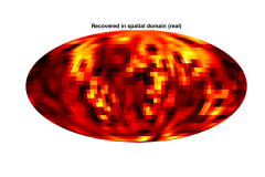
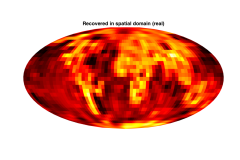
KKM Analysis, $M/L^{2}=0.3$ (15.8)	$M/L^{2}=0.5$ (25.8)	$M/L^{2}=1.0$ (64.3)
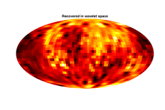
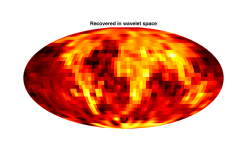
KKM Synthesis, $M/L^{2}=0.3$ (20.8)	$M/L^{2}=0.5$ (28.5)	$M/L^{2}=1.0$ (54.6)
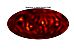
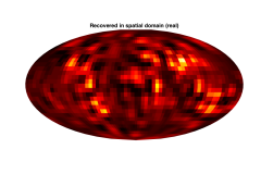
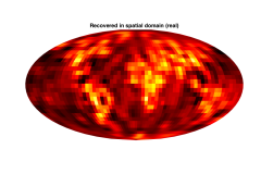
MW Analysis, $M/L^{2}=0.3$ (5.2)	$M/L^{2}=0.5$ (8.9)	$M/L^{2}=1.0(18.8)$	$M/L^{2}=1.9(59.8)$
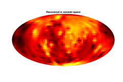
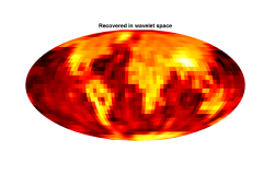
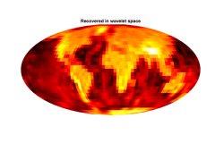
MW Synthesis, $M/L^{2}=0.3$ (26.2)	$M/L^{2}=0.5$ (31.9)	$M/L^{2}=1.0$ (42.0)	$M/L^{2}=1.9$ (76.4)
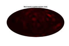
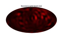
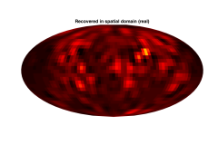
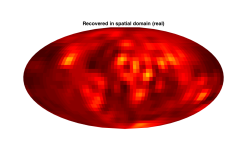
DH Analysis, $M/L^{2}=0.3$ (1.7)	$M/L^{2}=0.5$ (3.16)	$M/L^{2}=1.0$ (6.6)	$M/L^{2}=1.9$ (16.0)
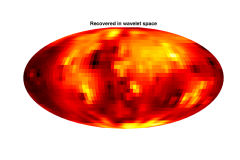
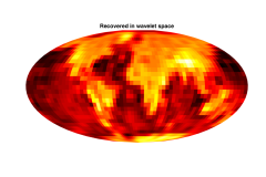
DH Synthesis, $M/L^{2}=0.3$ (26.1)	$M/L^{2}=0.5$ (31.2)	$M/L^{2}=1.0$ (41.7)	$M/L^{2}=1.9$ (62.8)

Figure 2: Reconstructed images from the low resolution inpainting experiment described in Sec. IV-A. The first two rows show the reconstruction using KKM sampling when solving the analysis and synthesis problems, respectively. The third and fourth rows are solutions to the same problems with MW sampling, and fifth and sixth rows correspond to DH sampling. Each column corresponds to a different number of measurements. The SNR for each image is giving in brackets in dB. The synthesis setting generally out-performs the analysis setting, while sampling schemes that require fewer samples generally out perform those requiring more samples.

IV Numerical Experiments

We perform numerical experiments to both assess the effectiveness of imposing sparsity in wavelet space and to test the impact of the sampling scheme used and whether or not the problem is solved in the analysis or synthesis setting.

We compare the analysis and synthesis settings for the KKM, DH and MW sampling schemes. These experiments are performed at low resolution as fast adjoint transforms for the DH and KKM sampling theorems are lacking. We chose to solve a noisy inpainting problem for these tests (as an example of a common inverse problem). At high resolution we demonstrate image reconstruction with both axisymmetric and directional wavelet sparsity priors using MW sampling (for which we have constructed fast adjoint operators). We test the method at high resolution on inpainting and deconvolution problems, and a combined inpainting and deconvolution problem, all in the presence of noise.

We generate low and high resolution test images from Earth topography data. The original Earth topography data are taken from the Earth Gravitational Model (EGM2008) publicly released by the U.S. National Geospatial-Intelligence Agency (NGA) EGM Development Team. The ground truth for the low and high resolution experiments performed in the remainder of this section are shown in Fig. 1.

Much of the work in this section takes advantage of publicly available codes: we use SSHT [52] and NSHT [53] to compute spherical harmonic transforms; SO3 [64] to compute harmonic transforms on the rotation group; S2LET [28, 30] to compute wavelet transforms on the sphere; and SOPT [47] to solve inverse problems.

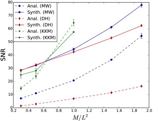
Figure 3: Reconstruction performance averaged over 10 realisations for the DH (red diamonds), MW (blue circles) and KKM (green stars) sampling schemes, when solving the low resolution inpainting problem in the analysis setting (dashed lines) and the synthesis setting (solid lines). The KKM and MW sampling schemes provide enhancements in reconstruction quality when compared to the DH sampling scheme. The synthesis setting is shown to be generally superior to the analysis setting.

The main code used to perform these experiments was not optimised and significant parts are run in serial in the high level language MATLAB. The runtimes for this naive implementation were as follows: the low resolution experiments described in Section IV-A take approximately 30 seconds for the MW sampling, 1 minute for the DH sampling, and 1 hour for the KKM sampling. The high resolution experiments performed with the MW sampling described in Section IV-B take around 10 minutes. All experiments were performed on a MacBook Pro (early 2015), with a 2.9 GHz Intel Core i5 processor and 16 GB of RAM.

IV-A Low Resolution Axisymmetric Experiments

We first solve a simple inpainting problem at low resolution ($L=32$) using axisymmetric wavelets ($N=1$). In this case the measurement operator in Eq. (30) is,

$$\boldsymbol{\mathsf{\Phi}}=\boldsymbol{\mathsf{\Phi}}_{\rm IP}\in\mathbb{R}^{M\times N_{\mathbb{S}^{2}}},$$ (35)

and represents a uniformly random masking of the spherical image, with one non-zero, unit value on each row specifying the location of the measured datum. The adjoint of the operator can be calculated trivially. Measurements are taken according to Eq. (30) with noise included corresponding to a signal-to-noise-ratio (SNR) of 46 dB, where ${\rm SNR}=20\log(\|\hat{\mbox{\boldmath${x}$}}\|_{2}/\|\hat{\mbox{\boldmath${x}$}}^{*}-\hat{\mbox{\boldmath${x}$}}\|_{2})$, defined in harmonic space to avoid differences due to the number of samples of each sampling scheme. We vary the number of measurements taken as $M=N_{\rm m}L^{2}$, where $N_{\rm m}=[0.3,0.5,1.0,1.5,1.9]$. We run these experiments for each of the sampling schemes we consider, specifically the KKM, MW and DH sampling schemes.

Results can be seen in Fig. 2. The improvement given by the lower number of samples of the KKM or MW sampling schemes can be seen clearly. There is also typically an improvement when solving Eq. (31), the synthesis problem, as opposed to Eq. (32), the analysis problem. We set $\eta=2.5$ (as we do for the remainder of the article unless otherwise stated), since this was shown to be the value resulting in the reconstructions of the highest SNR, although it should be noted that the resulting SNR was very similar for $2.5<\eta<4.5$ when an emperical investigation was conducted. In Fig. 3 we show the average SNR for 10 reconstructions, which supports the findings inferred from Fig. 2. These experiments were repeated on another data set from a different domain (natural light probe images) with similar results.

Acquired Data	Recovered Image Axisymmetric	Recovered Image Directional
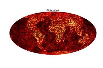
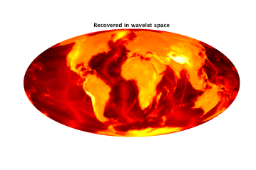
(a) Inpainting
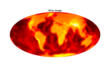
(b) Deconvolution
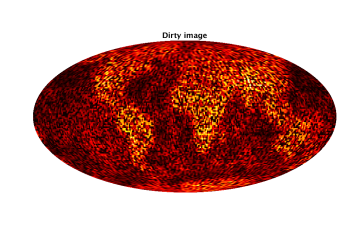
(c) Inpainting and deconvolution

Figure 4: Reconstructed images from the high resolution experiments described in Sec. IV-B. All problems are solved in the synthesis setting using MW sampling. Each solution is presented next to a band limited representation of the measured data. The SNR of the reconstructions are (a) 57.1 dB, (b) 51.8 dB and (c) 50.8 dB for the axisymmetric wavelets and (a) 58.4 dB, (b) 48.5 dB and (c) 48.5 dB for the directional wavelets. For the inpainting problem directional wavelets yield superior performance, while for the deconvolution and joint inpainting and deconvolution problems the SNR recovered with axisymmetric wavelets is superior, albeit visual artefacts are mitigated when using directional wavelets.

IV-B High Resolution Experiments

We run three example high resolution ($L=128$) experiments on the high resolution Earth map shown in Fig. 1. We solve all the problems with the MW sampling in the synthesis setting with $\eta=2.5$. We consider the MW sampling as there are currently no fast adjoint algorithms for the other sampling theorems and for the synthesis setting as it was shown to be superior in Sec. IV-A

We consider both axisymmetric wavelets ($N=1$) and directional wavelets with $N=4$ which leads to wavelets with odd azimuthal symmetry. Firstly, we solve a simple inpainting problem with a measurement operator given by Eq. (35), with $N_{m}=1.0$. Secondly, we consider a deconvolution problem, where the measurement operator is

$$\boldsymbol{\mathsf{\Phi}} = \boldsymbol{\mathsf{\Phi}}_{\rm CV}\in\mathbb{C}^{N_{\mathbb{S}^{2}}\times N_{\mathbb{S}^{2}}}$$ (36)

$$= \boldsymbol{\mathsf{Y}}\boldsymbol{\mathsf{G}}\tilde{\boldsymbol{\mathsf{Y}}},$$ (37)

where $\boldsymbol{\mathsf{G}}\in\mathbb{R}^{L^{2}\times L^{2}}$ is a diagonal matrix whose elements are,

$$\boldsymbol{\mathsf{G}}_{\ell m\ell^{\prime}m^{\prime}}=e^{-\ell^{2}\sigma^{2}}\delta_{\ell\ell^{\prime}}\delta_{mm^{\prime}},$$ (38)

where $\sigma=\pi/L$. Thirdly we solve the combined problem,

$$\boldsymbol{\mathsf{\Phi}}=\boldsymbol{\mathsf{\Phi}}_{\rm IP}\boldsymbol{\mathsf{\Phi}}_{\rm CV}.$$ (39)

We consider measurement noise with SNR of 46 dB.

We show the results of these experiments and a band limited version of the measured data in Fig. 4. The SNR of the recovered images are encouragingly high, showing a good similarity with the ground truth. The deconvolution problem shows minor visual artefacts in the axisymmetric wavelet case. The visual artefacts are reduced in the directional setting for the two problems involving deconvolution, however SNRs are slightly lower. The inpainting problem visually shows a marked improvement in the directional case over the axisymmetric case, as also illustrated by the improved SNR.

V Denoising Planck 353 GHz Data

The Planck satellite observed the entire sky at a range of microwave frequencies [1], yielding high resolution maps of the polarised Galactic dust emission from its high frequency polarised channel centred on 353 GHz and total intensity maps at even higher frequencies from other channels [68]. One of the many uses of these maps is the study of the Galactic magnetic field, where it is important to have high SNR maps of the clumps of dust in the Galaxy. It is common practise to smooth the data with a Gaussian kernel in order to suppress the high frequency noise [69]. This smoothing has the undesirable effect of not denoising large scales and, perhaps more damaging, removing important structure on small scales. Here we examine the use of sparsity in wavelet space as a prior to denoise the Planck 353GHz total intensity map.

The Planck 353 GHz data is available to download in HEALPix format [56]. We use the HEALPix software to compute the spherical harmonic coefficients of this spherical image. We then band limit these to $L=2048$ and use SSHT [52] to obtain a MW sampled image of the sphere. This is taken as our input data to then be denoised and can be seen in Fig. 5. An estimate of the noise level is made by downloading the noise maps from the same archive, performing the same operation, and averaging the noise over all of the sky. This leads to an initial estimate of $\epsilon$, which is subsequently optimised through experimentation.

We solve the denoising problem in the synthesis setting with measurement operator set to the identity and using the axisymmetric wavelets $(N=1)$. We set $\eta=3.0$ but have found the specific value have little effect on the reconstruction. Fig. 6 shows the original map, the result from denoising and a smoothed map. The smoothed map is the original map convolved with a 5 arcmin kernel to replicate the current denoising techniques adopted. It is clear the noise is reduced by our sparse denoising approach, while preserving small scale structure.

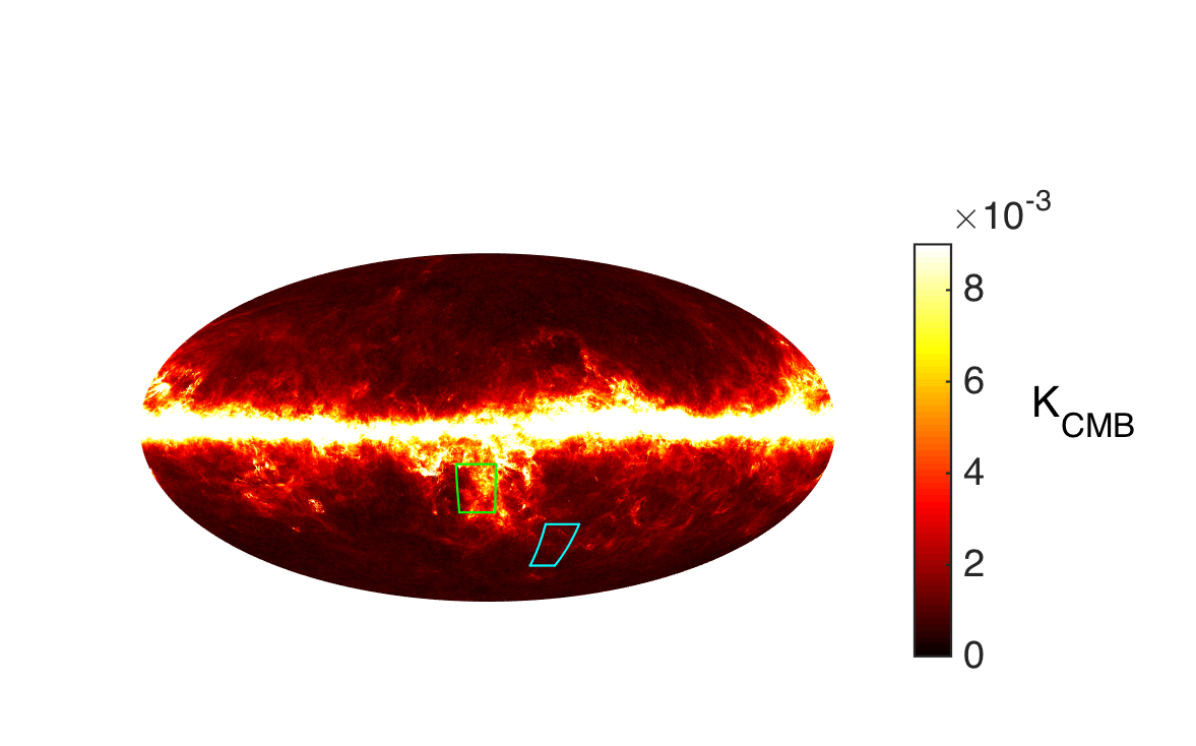
Figure 5: Acquired data of the 353 GHz Planck total intensity map. A full description of how this data was aquired can be found in Sec. V. The regions highlighted are shown in more detail in Figure 6.

Acquired Data	Recovered Image	Smoothed Image

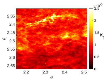
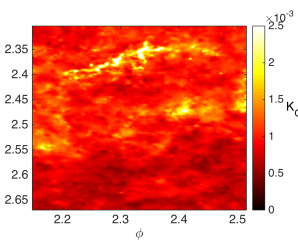
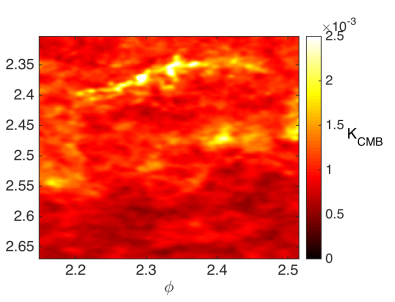
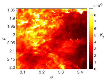
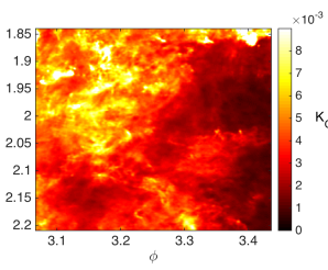
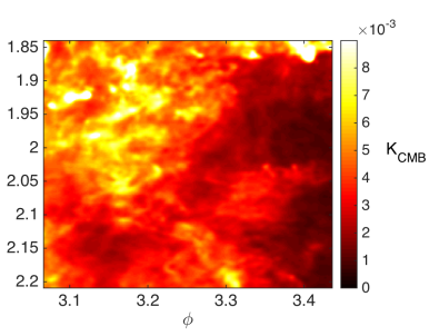
Figure 6: Results from denoising the Planck 353 GHz total intensity map. The left column shows the acquired data, the middle column shows the denoised data and the right column shows the data denoised by smoothing with a 5 arcmin Gaussian kernel (the standard approach [69]). Each plot shows a zoomed region of the sphere. The acquired data shown here is a zoom in of that shown in Fig. 5, the top figure is the blue region and the bottom figure is the green region.

VI Conclusions

We develop a general framework to solve image reconstruction problems on the sphere by sparse regularisation, minimising the $\ell_{1}$ norm of wavelet coefficient representations of spherical images. By developing fast adjoint operators, we recover convergence guarantees for the resulting convex optimisation problems. As examples, we have demonstrated that using our framework one can solve denoising, inpainting, and deconvolution problems effectively, and combinations thereof.

We study and compare the analysis and synthesis settings for solving inverse problems on the sphere for the first time. The analysis problem has shown promising results in Euclidean space, hypothesised to be due to its more restrictive nature. However, the more restrictive nature of the analysis framework in Euclidean space does not carry over to the spherical setting. The most restrictive solution-space on the sphere depends on the interplay between the adopted sampling scheme, the selection of the analysis/synthesis problem, and any weighting of the $\ell_{1}$ norm. We examine a variety of sampling schemes on the sphere, including the DH [51] and MW [52] sampling theorems (leading to theoretically exact spherical harmonic transforms) and the KKM [53] sampling scheme (leading to approximate but highly accurate spherical harmonic transforms). DH, MW and KKM sampling requires $\sim 4L^{2}$, $\sim 2L^{2}$, and $L^{2}$ samples, respectively.

To examine the analysis and synthesis problems and the impact of the various sampling schemes considered, we study results from a simple inpainting problem at low resolution. In the numerical results shown in Fig. 2 and Fig. 3 we find that the synthesis setting typically out-performs the analysis setting for suboptimal sampling schemes. Moreover, reconstruction fidelity is enhanced further by adopting more efficient sampling schemes that require fewer samples to capture the information content of signals on the sphere. These findings are robust to the choice of test signal.

We hypothesise that differences between the analysis and synthesis settings on the sphere are due to restrictions of the solution-space. Elad et al. [43] showed theoretically and with simulations that there are fundamental differences between the analysis and synthesis settings due to the solution-spaces. As in Euclidean space, we find settings with a more restricted solution-space yield superior performance. In contrast to Euclidean space, it is the synthesis setting rather than the analysis setting that typically results in a more restrictive solution-space on the sphere. This is due to the inefficiency of spherical sampling schemes and the weighting introduced in the $\ell_{1}$ norm. Since the KKM sampling exhibits the optimal number of samples on the sphere there is no appreciable different between the size of the solution-spaces of the analysis and synthesis problems and the fidelity of spherical images recovered by the analysis and synthesis approaches are similar. In addition, the sparsity of band-limited signals is further promoted by more efficient sampling schemes when considering a sparse representation that captures spatial localisation [50], such as wavelets.

We also demonstrate solving inverse problems in a number of high resolution settings, facilitated by our fast adjoint operators. We solve inpainting, deconvolution, and combined inpainting and deconvolution problems, all in the presence of noise, using both axisymmetric and directional wavelets. For all inverse problems considered our sparse regularisation techniques yield excellent reconstruction fidelity.

Our framework for solving inverse problems on the sphere can be applied to many real-world problems. We have shown that our framework can be used to effectively denoise 353 GHz channel observations from the Planck satellite, which will be useful for studying Galactic magnetic fields.

Appendix A Fast Wigner Transform Adjoints

Standard convex optimisation methods require not only the application of the operators that appear in the optimisation problem but also their adjoints. Moreover, these methods are typically iterative, necessitating repeated application of each operator and its adjoint. Thus, to solve optimisation problems that incorporate Wigner transform operators fast algorithms to apply both the operator and its adjoint are required to render high-resolution problems computationally feasible.

Here we develop fast algorithms to perform adjoint forward and adjoint inverse Wigner transforms for the extension of the MW sampling scheme to the rotation group [64]. The fast adjoint follows by taking the adjoint of each stage of the fast standard transforms [64] and applying these in reverse order. The forward and inverse transforms can be found in [64, Sec. 3]. Here we use notation consistent with that work, where $\Delta_{{m^{\prime}}{m}}^{\ell}=D_{mn}^{\ell}(0,\pi/2,0)$. The fast adjoint of the forward transform is as follows:

$$G_{mnm^{\prime}}^{\dagger} ={\rm i}^{-(m-n)}\sum_{\ell=0}^{L-1}\Delta_{{m^{\prime}}{m}}^{\ell}\>\Delta_{{m^{\prime}}{n}}^{\ell}\>{f}^{\ell}_{{m}{n}}\>,$$ (40)

$$\tilde{G}_{mnm^{\prime}{}^{\prime}}^{\dagger} =(2\pi)^{2}\sum_{m^{\prime}=-({L}-1)}^{{L}-1}G_{mnm^{\prime}}^{\dagger}\>w(m^{\prime}-m^{\prime}{}^{\prime})\>,$$ (41)

$$\tilde{G}_{mn}^{\dagger}(\beta_{b}) =\frac{1}{2L-1}\sum_{m^{\prime}=-(L-1)}^{L-1}\tilde{G}_{mnm^{\prime}}^{\dagger}e^{{\rm i}m^{\prime}\beta_{b}}$$ (42)

$$F_{mn}^{\dagger}(\beta_{b}) =\begin{cases}\>\tilde{G}_{mn}^{\dagger}(\beta_{b})+(-1)^{m+n}\tilde{G}_{mn}^{\dagger}(-\beta_{b})\>,\\ &\!\!\!\!\!\!\!\!\!\!\!\!\!\!\!\!\!\!\!\!\!\!\!\!\!\!\!\!\!\!\!\!\!\!\!\!b\in\{0,1,\dots,L-2\}\\ \>\tilde{G}_{mn}^{\dagger}(\beta_{b})\>,&\!\!\!\!\!\!\!\!\!\!\!\!\!\!\!\!\!\!\!\!\!\!\!\!\!\!\!\!\!\!\!\!\!\!\!\!b=L-1\\ \end{cases}$$ (43)

$$f^{\dagger}(\alpha_{a},\beta_{b},\gamma_{g}) =\frac{1}{(2M-1)(2N-1)}$$

$$\sum_{n=-(N-1)}^{N-1}\sum_{m=-(M-1)}^{M-1}F_{mn}^{\dagger}(\beta_{b})e^{{\rm i}(m\alpha_{a}+n\gamma_{g})}.$$ (44)

Similarly, the fast adjoint of the inverse transform is as follows:

$$\tilde{f}(\alpha_{a},\beta_{b},\gamma_{g})=\begin{cases}f(\alpha_{a},\beta_{b},\gamma_{g}),&t\in\{0,1,\dotsc,{L}-1\}\\ 0\>,&t\in\{{L},\dotsc,2{L}-2\}\end{cases}\>,$$ (45)

$$F^{\dagger}_{mnm^{\prime}} =\sum_{a=0}^{2M-2}\sum_{b=0}^{L-1}\sum_{g=0}^{2N-2}\tilde{f}(\alpha_{a},\beta_{b},\gamma_{g})e^{-{\rm i}(m\alpha_{a}+n\beta_{b}+m^{\prime}\gamma_{g})}$$ (46)

$${f}^{\ell\dagger}_{{m}{n}} ={\rm i}^{-(n-m)}\!\!\!\!\!\!\!\sum_{m^{\prime}=-(L-1)}^{L-1}\!\!\!\!\frac{2\ell+1}{8\pi^{2}}\Delta_{{m^{\prime}}{m}}^{\ell}\>\Delta_{{m^{\prime}}{n}}^{\ell}\>F_{mnm^{\prime}}^{\dagger}.$$ (47)

These fast adjoint algorithms scale as $\mathcal{O}(NL^{3})$ (where $N\ll L\sim M$) and are implemented in the SO3 code.

References

- [1] Planck Collaboration I, “Planck 2015 results. I. Overview of products and scientific results,” Astron. & Astrophys., submitted, Feb. 2015.
- [2] H. Johansen-Berg and T. E. J. Behrens, Diffusion MRI: From quantitative measurement to in-vivo neuroanatomy. San Diego: Academic Press, 2009.
- [3] F. J. Narcowich and J. D. Ward, “Non-stationary wavelets on the m-sphere for scattered data,” Applied Comput. Harm. Anal., vol. 3, pp. 324–336, 1996.
- [4] D. Potts and M. Tasche, “Interpolatory wavelets on the sphere,” in Approximation Theory VIII, 1995, pp. 335–342.
- [5] W. Freeden and U. Windheuser, “Combined spherical harmonic and wavelet expansion – a future concept in the Earth’s gravitational determination,” Applied Comput. Harm. Anal., vol. 4, pp. 1–37, 1997.
- [6] B. Torrésani, “Position-frequency analysis for signals defined on spheres,” Signal Proc., vol. 43, pp. 341–346, 1995.
- [7] S. Dahlke and P. Maass, “Continuous wavelet transforms with applications to analyzing functions on sphere,” J. Fourier Anal. and Appl., vol. 2, pp. 379–396, 1996.
- [8] M. Holschneider, “Continuous wavelet transforms on the sphere,” J. Math. Phys., vol. 37, pp. 4156–4165, 1996.
- [9] J.-P. Antoine and P. Vandergheynst, “Wavelets on the 2-sphere: a group theoretical approach,” Applied Comput. Harm. Anal., vol. 7, pp. 1–30, 1999.
- [10] J.-P. Antoine and P. Vandergheynst, “Wavelets on the n-sphere and related manifolds,” J. Math. Phys., vol. 39, no. 8, pp. 3987–4008, 1998.
- [11] Y. Wiaux, L. Jacques, and P. Vandergheynst, “Correspondence principle between spherical and Euclidean wavelets,” Astrophys. J., vol. 632, pp. 15–28, 2005.
- [12] J. L. Sanz, D. Herranz, M. López-Caniego, and F. Argüeso, “Wavelets on the sphere – application to the detection problem,” in EUSIPCO, Sept. 2006.
- [13] J. D. McEwen, M. P. Hobson, and A. N. Lasenby, “A directional continuous wavelet transform on the sphere,” ArXiv, 2006.
- [14] P. Schröder and W. Sweldens, “Spherical wavelets: efficiently representing functions on the sphere,” in Computer Graphics Proceedings (SIGGRAPH ‘95), 1995, pp. 161–172.
- [15] R. B. Barreiro, M. P. Hobson, A. N. Lasenby, A. J. Banday, K. M. Górski, and G. Hinshaw, “Testing the Gaussianity of the COBE-DMR data with spherical wavelets,” Mon. Not. Roy. Astron. Soc., vol. 318, pp. 475–481, 2000.
- [16] I. Bogdanova, P. Vandergheynst, J.-P. Antoine, L. Jacques, and M. Morvidone, “Stereographic wavelet frames on the sphere,” Applied Comput. Harm. Anal., vol. 19, no. 2, pp. 223–252, 2005.
- [17] J. D. McEwen and A. M. M. Scaife, “Simulating full-sky interferometric observations,” Mon. Not. Roy. Astron. Soc., vol. 389, no. 3, pp. 1163–1178, 2008.
- [18] J. D. McEwen, Y. Wiaux, and D. M. Eyers, “Data compression on the sphere,” Astron. & Astrophys., vol. 531, p. A98, 2011.
- [19] W. Sweldens, “The lifting scheme: a construction of second generation wavelets,” SIAM J. Math. Anal., vol. 29, no. 2, pp. 511–546, 1997.
- [20] J. Delabrouille, J.-F. Cardoso, M. Le Jeune, M. Betoule, G. Fay, and F. Guilloux, “A full sky, low foreground, high resolution CMB map from WMAP,” Astron. & Astrophys., vol. 493, pp. 835–857, Jan. 2009.
- [21] J. Bobin, J.-L. Starck, F. Sureau, and S. Basak, “Sparse component separation for accurate cosmic microwave background estimation,” Astron. & Astrophys., vol. 550, p. A73, Feb. 2013.
- [22] K. K. Rogers, H. V. Peiris, B. Leistedt, J. D. McEwen, and A. Pontzen, “SILC: a new Planck internal linear combination CMB temperature map using directional wavelets,” Mon. Not. Roy. Astron. Soc., in press, 2016.
- [23] K. K. Rogers, H. V. Peiris, B. Leistedt, J. D. McEwen, and A. Pontzen, “Spin-SILC: CMB polarisation component separation with spin wavelets,” Mon. Not. Roy. Astron. Soc., submitted, 2016.
- [24] F. J. Narcowich, P. Petrushev, and J. D. Ward, “Localized tight frames on spheres,” SIAM J. Math. Anal., vol. 38, no. 2, pp. 574–594, 2006.
- [25] P. Baldi, G. Kerkyacharian, D. Marinucci, and D. Picard, “Asymptotics for spherical needlets,” Ann. Stat., vol. 37 No.3, pp. 1150–1171, 2009.
- [26] D. Marinucci, D. Pietrobon, A. Balbi, P. Baldi, P. Cabella, G. Kerkyacharian, P. Natoli, D. Picard, and N. Vittorio, “Spherical needlets for cosmic microwave background data analysis,” Mon. Not. Roy. Astron. Soc., vol. 383, pp. 539–545, 2008.
- [27] Y. Wiaux, J. D. McEwen, P. Vandergheynst, and O. Blanc, “Exact reconstruction with directional wavelets on the sphere,” Mon. Not. Roy. Astron. Soc., vol. 388, no. 2, pp. 770–788, 2008.
- [28] B. Leistedt, J. D. McEwen, P. Vandergheynst, and Y. Wiaux, “S2LET: A code to perform fast wavelet analysis on the sphere,” Astron. & Astrophys., vol. 558, no. A128, pp. 1–9, 2013.
- [29] J. D. McEwen, P. Vandergheynst, and Y. Wiaux, “On the computation of directional scale-discretized wavelet transforms on the sphere,” in SPIE Wavelets and Sparsity XV, vol. 8858, 2013.
- [30] J. D. McEwen, B. Leistedt, M. Büttner, H. V. Peiris, and Y. Wiaux, “Directional spin wavelets on the sphere,” IEEE Trans. Sig. Proc., submitted, 2015.
- [31] J. D. McEwen, “Ridgelet transform on the sphere,” IEEE Trans. Sig. Proc., submitted, 2015.
- [32] J. Y. H. Chan, B. Leistedt, T. D. Kitching, and J. D. McEwen, “Second-generation curvelets on the sphere,” IEEE Trans. Sig. Proc., submitted, 2015.
- [33] J. D. McEwen, C. Durastanti, and Y. Wiaux, “Localisation of directional scale-discretised wavelets on the sphere,” Applied and Computational Harmonic Analysis, pp. –, 2016. [Online]. Available: http://www.sciencedirect.com/science/article/pii/S1063520316000324
- [34] J.-L. Starck, Y. Moudden, P. Abrial, and M. Nguyen, “Wavelets, ridgelets and curvelets on the sphere,” Astron. & Astrophys., vol. 446, pp. 1191–1204, Feb. 2006.
- [35] C. Durastanti, Y. Fantaye, F. Hansen, D. Marinucci, and I. Z. Pesenson, “Simple proposal for radial 3D needlets,” Phys. Rev. D., vol. 90, no. 10, p. 103532, Nov. 2014.
- [36] B. Leistedt and J. D. McEwen, “Exact wavelets on the ball,” IEEE Trans. Sig. Proc., vol. 60, no. 12, pp. 6257–6269, 2012.
- [37] J. D. McEwen and B. Leistedt, “Fourier-Laguerre transform, convolution and wavelets on the ball,” in 10th International Conference on Sampling Theory and Applications (SampTA), 2013, pp. 329–333.
- [38] B. Leistedt, J. D. McEwen, T. D. Kitching, and H. V. Peiris, “3D weak lensing with spin wavelets on the ball,” Phys. Rev. D., vol. 92, no. 12, p. 123010, Dec. 2015.
- [39] F. Lanusse, A. Rassat, and J.-L. Starck, “Spherical 3D isotropic wavelets,” Astron. & Astrophys., vol. 540, p. A92, Apr. 2012.
- [40] E. Candès, J. Romberg, and T. Tao, “Robust uncertainty principles: exact signal reconstruction from highly incomplete frequency information,” IEEE Trans. Inform. Theory, vol. 52, no. 2, pp. 489–509, feb 2006.
- [41] E. Candès, “Compressive sampling,” in Proc. Int. Congress Math., ser. Euro. Math. Soc., vol. III, 2006, p. 1433.
- [42] D. Donoho, “Compressed sensing,” IEEE Trans. Inform. Theory, vol. 52, no. 4, pp. 1289–1306, apr 2006.
- [43] M. Elad, P. Milanfar, and R. Rubinstein, “Analysis versus synthesis in signal priors,” Inv. Prob., vol. 23, pp. 947–968, 2007.
- [44] N. Cleju, M. G. Jafari, and M. D. Plumbley, “Choosing analysis or synthesis recovery for sparse reconstruction,” in Signal Processing Conference (EUSIPCO), 2012 Proceedings of the 20th European, Aug 2012, pp. 869–873.
- [45] S. Nam, M. E. Davies, M. Elad, and R. Gribonval, “The cosparse analysis model and algorithms,” Applied Comput. Harm. Anal., vol. 34, no. 1, pp. 30–56, June 2013.
- [46] R. E. Carrillo, J. D. McEwen, and Y. Wiaux, “Sparsity averaging reweighted analysis (SARA): a novel algorithm for radio-interferometric imaging,” Mon. Not. Roy. Astron. Soc., vol. 426, no. 2, pp. 1223–1234, 2012.
- [47] R. E. Carrillo, J. D. McEwen, D. V. D. Ville, J.-P. Thiran, and Y. Wiaux, “Sparsity averaging for compressive imaging,” IEEE Sig. Proc. Let., vol. 20, no. 6, pp. 591–594, 2013.
- [48] P. Abrial, Y. Moudden, J.-L. Starck, B. Afeyan, J. Bobin, J. Fadili, and M. K. Nguyen, “Morphological component analysis and inpainting on the sphere: application in physics and astrophysics,” J. Fourier Anal. and Appl., vol. 14, no. 6, pp. 729–748, 2007.
- [49] H. Rauhut and R. Ward, “Sparse recovery for spherical harmonic expansions,” in SampTA, 2011.
- [50] J. D. McEwen, G. Puy, J.-P. Thiran, P. Vandergheynst, D. V. D. Ville, and Y. Wiaux, “Sparse image reconstruction on the sphere: implications of a new sampling theorem,” IEEE Trans. Image Proc., vol. 22, no. 6, pp. 2275–2285, 2013.
- [51] J. R. Driscoll and D. M. J. Healy, “Computing Fourier transforms and convolutions on the sphere,” Adv. Appl. Math., vol. 15, pp. 202–250, 1994.
- [52] J. D. McEwen and Y. Wiaux, “A novel sampling theorem on the sphere,” IEEE Trans. Sig. Proc., vol. 59, no. 12, pp. 5876–5887, 2011.
- [53] Z. Khalid, R. A. Kennedy, and J. D. McEwen, “An optimal-dimensionality sampling scheme on the sphere with fast spherical harmonic transforms,” IEEE Trans. Sig. Proc., vol. 62, no. 17, pp. 4597–4610, 2014.
- [54] S. M. Feeney, D. Marinucci, J. D. McEwen, H. V. Peiris, B. D. Wandelt, and V. Cammarota, “Sparse inpainting and isotropy,” JCAP, vol. 1, p. 050, Jan. 2014.
- [55] D. M. J. Healy, D. Rockmore, P. J. Kostelec, and S. S. B. Moore, “FFTs for the 2-sphere – improvements and variations,” J. Fourier Anal. and Appl., vol. 9, no. 4, pp. 341–385, 2003.
- [56] K. M. Górski, E. Hivon, A. J. Banday, B. D. Wandelt, F. K. Hansen, M. Reinecke, and M. Bartelmann, “Healpix – a framework for high resolution discretization and fast analysis of data distributed on the sphere,” Astrophys. J., vol. 622, pp. 759–771, 2005.
- [57] R. G. Crittenden and N. G. Turok, “Exactly azimuthal pixelizations of the sky,” ArXiv, 1998.
- [58] A. G. Doroshkevich, P. D. Naselsky, O. V. Verkhodanov, D. I. Novikov, V. I. Turchaninov, I. D. Novikov, P. R. Christensen, and L. Y. Chiang, “Gauss–Legendre Sky Pixelization (GLESP) for CMB maps,” Int. J. Mod. Phys. D., vol. 14, no. 2, pp. 275–290, 2005.
- [59] S. Deslauriers-Gauthier and P. Marziliano, “Sampling signals with a finite rate of innovation on the sphere,” IEEE Transactions on Signal Processing, vol. 61, no. 18, pp. 4552–4561, 2013.
- [60] I. Dokmanić and Y. M. Lu, “Sampling sparse signals on the sphere: Algorithms and applications,” IEEE Transactions on Signal Processing, vol. 64, no. 1, pp. 189–202, 2016.
- [61] Y. Sattar, Z. Khalid, and R. A. Kennedy, “Accurate Reconstruction of Finite Rate of Innovation Signals on the Sphere,” ArXiv e-prints, Dec. 2016.
- [62] D. A. Varshalovich, A. N. Moskalev, and V. K. Khersonskii, Quantum theory of angular momentum. Singapore: World Scientific, 1989.
- [63] P. Kostelec and D. Rockmore, “FFTs on the rotation group,” J. Fourier Anal. and Appl., vol. 14, pp. 145–179, 2008.
- [64] J. D. McEwen, M. Buttner, B. Leistedt, H. V. Peiris, and Y. Wiaux, “A novel sampling theorem on the rotation group,” IEEE Signal Processing Letters, vol. 22, pp. 2425–2429, Dec. 2015.
- [65] Z. Khalid, S. Durrani, R. A. Kennedy, Y. Wiaux, and J. D. McEwen, “Gauss-Legendre sampling on the rotation group,” IEEE Signal Processing Letters, vol. 23, pp. 207–211, Feb. 2016.
- [66] A. Bronstein, Y. Choukroun, R. Kimmel, and M. Sela, “Consistent discretization and minimization of the L1 Norm on Manifolds,” ArXiv e-prints, Sept. 2016.
- [67] P. Combettes and J.-C. Pesquet, Proximal splitting methods in signal processing. New York: Springer, 2011.
- [68] Planck Collaboration XXIX, “Planck intermediate results. XXIX. All-sky dust modelling with Planck, IRAS, and WISE observations,” Astron. & Astrophys., vol. 586, p. A132, Feb. 2016.
- [69] Planck Collaboration XXXII, “Planck intermediate results. XXXII. The relative orientation between the magnetic field and structures traced by interstellar dust,” Astron. & Astrophys., vol. 586, p. A135, Feb. 2016.