Trace test

Anton Leykin Anton Leykin
School of Mathematics
Georgia Institute of Technology
686 Cherry Street
Atlanta, GA 30332-0160 USA
USA
leykin@math.gatech.edu http://people.math.gatech.edu/ aleykin3
Jose Israel Rodriguez Jose Israel Rodriguez
Department of Statistics
University of Chicago
Chicago, IL 60637
USA
JoIsRo@uchicago.edu http://home.uchicago.edu/j̃oisro
 and  Frank Sottile Frank Sottile
Department of Mathematics
Texas A&M University
College Station
Texas  77843
USA
sottile@math.tamu.edu http://www.math.tamu.edu/ sottile
Abstract.

The trace test in numerical algebraic geometry verifies the completeness of a witness set of an irreducible variety in affine or projective space. We give a brief derivation of the trace test and then consider it for subvarieties of products of projective spaces using multihomogeneous witness sets. We show how a dimension reduction leads to a practical trace test in this case involving a curve in a low-dimensional affine space.

Key words and phrases:
trace test, witness set, numerical algebraic geometry
1991 Mathematics Subject Classification:
65H10
Research of Leykin supported in part by NSF grant DMS-1151297
Research of Rodriguez supported in part by NSF grant DMS-1402545
Research of Sottile supported in part by NSF grant DMS-1501370

Introduction

Numerical algebraic geometry [11] uses numerical analysis to study algebraic varieties, which are sets defined by polynomial equations. It is becoming a core tool in applications of algebraic geometry outside of mathematics. Its fundamental concept is a witness set, which is a general linear section of an algebraic variety [8]. This gives a representation of a variety which may be manipulated on a computer and forms the basis for many algorithms. The trace test is used to verify that a witness set is complete.

We illustrate this with the folium of Descartes, defined by $x^{3}+y^{3}=3xy$. A general line $\ell$ meets the folium in three points $W$ and the pair $(W,\ell)$ forms a witness set for the folium. Tracking the points of $W$ as $\ell$ moves computes witness sets on other lines. Figure 1 shows these witness sets on four parallel lines.

Figure 1. Witness sets and the trace test for the folium of Descartes

It also shows the average of each witness set, which is one-third of their sum, the trace. The four traces are collinear.

Any subset $W^{\prime}$ of $W$ may be tracked to get a corresponding subset on any other line, and we may consider the traces of the subsets as $\ell$ moves in a pencil. The traces are collinear if and only if $W^{\prime}$ is complete in that $W^{\prime}=W$. This may also be seen in Figure 1. This trace test [10] is used to verify the completeness of a subset of a witness set.

Methods to check linearity of a univariate function—e.g., the trace—in the context of algorithms for numerical algebraic geometry were recently discussed in [2].

An algebraic variety $V$ may be the union of other varieties, called its components. Given a witness set $W=V\cap L$ for $V$ ($L$ is a linear space), numerical irreducible decomposition [9] partitions $W$ into subsets corresponding to the components of $V$. For example, suppose that $V=E\cup F$ is the union of the ellipse $8(x+1)^{2}+3(2y+x+1)^{2}=8$ and the folium, as in Figure 2.


Figure 2. Numerical irreducible decomposition for the ellipse and folium

A witness set for $V$ consists of the five points $W=V\cap\ell$. Tracking points of $W$ as $\ell$ varies in a loop in the space of lines, a point $w\in W$ may move to a different point which lies in the same component of $V$. Doing this for several loops partitions $W$ into two sets, of cardinalities two and three, respectively. Applying the trace test to each subset verifies that each is a witness set of a component of $V$.

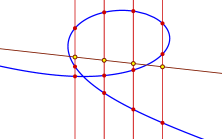
A multiprojective variety is subvariety of a product of projective spaces. Since there are different types of general linear sections in a product of projective spaces, a witness set for a multiprojective variety is necessarily a collection of such sections, called a witness collection. We see this in Figure 3, where vertical and horizontal lines are the two types of hyperplanes in the product ${\mathbb{P}}^{1}\times{\mathbb{P}}^{1}$.

Refer to caption$-2$ $1$ $y$ $1$ $2$ $x$ ${\ell^{(2)}}$ $\ell$ ${\ell^{(1)}}$ $C$ $C$
Refer to caption$-2$ $1$ $z=\frac{1}{y}$ $1$ $2$ $3$ $x$ ${\ell^{(2)}}$ $\ell$ $\ell$ ${\ell^{(1)}}$ $C$
Figure 3. The curve $C$ in ${\mathbb{P}}^{1}\times{\mathbb{P}}^{1}$ is defined by $xy^{2}=1$ and $x=z^{2}=(1/y)^{2}$ in two distinct affine charts ${\mathbb{C}}\times{\mathbb{C}}$. Its witness collection is $((W_{1},\ell^{(1)}),(W_{2},\ell^{(2)}))$, where $W_{i}=C\cap\ell^{(i)}$.

Witness sets for multihomogeneous varieties were introduced in [4]. Figure 3 shows that the trace obtained by varying $\ell^{(2)}$ is nonlinear in either affine chart. One may instead apply the trace test to a witness set in the ambient projective space of the Segre embedding. By Remark 10, this may involve very large witness sets. We propose an alternative method to verify irreducible components, using a dimension reduction that sidesteps this potential bottleneck followed by the ordinary trace test in an affine patch on the product of projective spaces. In Figure 3 this is represented by the linear section of the plane cubic $xy^{2}=1$ by the line $\ell$. Both $xy^{2}=1$ and $x=z^{2}=(\frac{1}{y})^{2}$ bihomogenize to the same cubic, but line $\ell$ in the first affine chart becomes a quadric in the second. Moreover, a general line in the second chart intersects the curve at two points. Taking a generic chart preserves the total degree, so we first choose a chart, and then take a general linear section in that chart. This will have the same number of points as the the total number of points in the witness collection.

In §1 we present a simple derivation of the usual trace test in affine space. While containing the same essential ideas as in [10], our derivation is shorter, and we believe significantly clearer. In §2 we introduce witness collections, collections of multihomogeneous witness sets representing multiprojective varieties. In §3 we present trace test for multihomogeneous varieties that exploits a reduction in dimension. Proofs are placed in §4 to streamline the exposition.

1. Trace in an affine space

We derive the trace test for curves in affine space, which verifies the completeness of a witness set. We also show how to reduce to a curve when the variety has greater dimension. Let ${\color[rgb]{0,0,1}V}\subset{\mathbb{C}}^{n}$ be an irreducible algebraic variety of dimension $m>0$. We restrict to $m>0$, for if $m=0$, then $V$ is a single point. Let $(x,y)$ be coordinates for ${\mathbb{C}}^{n}$ with $x\in{\mathbb{C}}^{n-m}$ and $y\in{\mathbb{C}}^{m}$. Polynomials defining $V$ generate a prime ideal $I$ in the polynomial ring ${\mathbb{C}}[x,y]$. We assume that $V$ is in general position with respect to these coordinates. In particular, the projection $\pi$ of $V$ to ${\mathbb{C}}^{m}$ is a branched cover with a fiber of ${\color[rgb]{0,0,1}d}=\deg V$ points outside the ramification locus ${\color[rgb]{0,0,1}\Delta}\subset{\mathbb{C}}^{m}$.

Example 1.

If we project the folium of Descartes to the $y$-axis, all fibers consist of three points, except those above zeroes of the discriminant $-27y^{3}(y^{3}-4)$. These zeroes form the ramification locus $\Delta=\{0,2^{2/3},(-\frac{1}{2}\pm\frac{\sqrt{-3}}{2})2^{2/3}\}$.

Refer to caption00$2^{2/3}$ $y$
Figure 4. Projecting the folium to the $y$-axis.

Figure 4 shows the real points, where the fiber consists of one or three points, with this number changing at the real points of $\Delta$.

Let ${\color[rgb]{0,0,1}\ell}\subset{\mathbb{C}}^{m}$ be a general line parameterized by $t\in{\mathbb{C}}$, so that ${\color[rgb]{0,0,1}L}:={\mathbb{C}}^{n-m}\times\ell$ is a general affine subspace of dimension $n{-}m{+}1$ with coordinates $(x,t)$. The intersection ${\color[rgb]{0,0,1}C}:=V\cap L$ is an irreducible curve of degree $d$ by Bertini’s Theorem (see Theorem 12) and the projection $\pi\,\colon C\to\ell$ is a degree $d$ cover over $\ell\smallsetminus\Delta$.

Proposition 2.

Let $C\subset{\mathbb{P}}^{n}$, $n\geq 2$, be a curve. Let $\alpha\,\colon{\mathbb{P}}^{n}\dashedrightarrow{\mathbb{P}}^{2}$ be a generic projection. Then $C$ is irreducible if and only if $\alpha(C)$ is irreducible.

Note that one can state Proposition 2 for a generic linear map of affine spaces ${\mathbb{C}}^{n}\to{\mathbb{C}}^{2}$, since taking affine charts preserves (ir)reducibility.

Since $V$ and $L$ are in general position, Proposition 2 implies that the projection of $C$ to the $(x_{i},t)$-coordinate plane is an irreducible curve given by a single polynomial $f(x_{i},t)$ of degree $d$ with all monomials up to degree $d$ having nonzero coefficients.

Normalize $f$ so that the coefficient of $x_{i}^{d}$ is $1$, and extend scalars from ${\mathbb{C}}$ to ${\mathbb{C}}(t)$. Then $f\in{\mathbb{C}}(t)[x_{i}]$ is a monic irreducible polynomial in $x_{i}$. The negative sum of its roots is the coefficient of $x_{i}^{d-1}$ in $f$, which is an affine function of $t$. Equivalently,

$$\operatorname{tr}_{K/{\mathbb{C}}(t)}(x_{i})\ =\ c_{0}t+c_{1}\,,\quad(\mbox{for some }c_{0},c_{1}\in{\mathbb{C}})\,,$$

where $K$ is a finite extension of ${\mathbb{C}}(t)$ containing the roots of $f$. A function of $t$ of the form $c_{0}t+c_{1}$ where $c_{0},c_{1}$ are constants is an affine function. We deduce the following.

Proposition 3.

The sum in ${\mathbb{C}}^{n-m}$ of the points in a fiber of $C$ over $t\in\ell\smallsetminus\Delta$ is an affine function of $t$.

The converse to this holds.

Proposition 4.

No proper subset of the points in a fiber of $C$ over $t\in\ell\smallsetminus\Delta$ has sum that is an affine function of $t$.

Example 5.

Consider this for the folium of Descartes. As the folium is a plane curve, a general projection $\alpha$ of Proposition 2 is a general change of coordinates. In the coordinates $\xi=x+1$ and $t=2y-x$, the folium has equation

$$9\xi^{3}+(3t-39)\xi^{2}+(3t^{2}-18t+51)\xi+t^{3}-3t^{2}+15t-21\ =\ 0\,.$$

The trace is $-\frac{t}{3}+\frac{13}{3}$. Figure 5 shows Figure 1 under this change of coordinates.

Refer to caption
Figure 5. Folium of Descartes in new coordinates

The lines become vertical, and the average of the trace is the line $\xi=-\frac{t}{9}+\frac{13}{9}$.

Remark 6.

We generalize the situation of Proposition 4. A pencil of linear spaces is a family $M_{t}$ for $t\in{\mathbb{C}}$ of linear spaces that depends affinely on the parameter $t$. Each $M_{t}$ is the span of a linear space $L$ and a point $t$ on a line $\ell$ that is disjoint from $L$.

Suppose that $V\subset{\mathbb{P}}^{n}$ is a subvariety of dimension $m$ and that $M_{t}$ for $t\in{\mathbb{C}}$ is a general pencil of linear subspaces of codimension $m$ with $V\cap M_{0}$ transverse. Let $\Delta\subset{\mathbb{C}}$ be the finite set of points $t$ such that the intersection $V\cap M_{t}$ is not transverse. Given any path $\gamma\,\colon[0,1]\to{\mathbb{C}}\smallsetminus\Delta$ with $\gamma(0)=0$ and any $v\in V\cap M_{0}$, we may analytically continue $v$ along $\gamma$ to obtain a path $v(\gamma(s))$ for $s\in[0,1]$ with $v(\gamma(s))\in V\cap M_{\gamma(s)}$.

The sum of the points in a subset $W$ of $V\cap M_{0}$ is an affine function of $t$ if for a nonconstant path $\gamma\,\colon[0,1]\to{\mathbb{C}}\smallsetminus\Delta$ with $\gamma(0)=0$, the sum of the points $w(\gamma(s))$ is an affine function of $\gamma(s)$. This is independent of choice of path and of a general pencil.

Remark 7.

This leads to the trace test. Let $V\subset{\mathbb{P}}^{n}$ (or ${\mathbb{C}}^{n}$) be a possibly reducible variety of dimension $m$ and $M$ a general linear space of codimension $m$ so that $W=V\cap M$ is a witness set for $V$. Suppose we have a subset $\emptyset\neq W^{\prime}\subset W$ whose points lie in a single component $V^{\prime}$ of $V$ so that $W^{\prime}\subset V^{\prime}\cap M$. Such a set $W^{\prime}$ is a partial witness set for $V^{\prime}$. To test if $W^{\prime}=V^{\prime}\cap M$, let $M_{t}$ for $t\in{\mathbb{C}}$ be a general pencil of codimension $m$ planes in ${\mathbb{P}}^{n}$ with $M=M_{0}$ and test if the sum of the points of $W^{\prime}$ is an affine function of $t$. By Proposition 4, $W^{\prime}=V^{\prime}\cap M$ if and only if it passes this trace test.

Remark 8.

Let $U$ be a variety and $\phi\,\colon U\dashedrightarrow{\mathbb{P}}^{n}$ be a rational map with image $V=\overline{\phi(U)}$. As obtaining defining equations for $V$ may not be practical, working with a witness set $V\cap M$ may not be feasible. Instead one may work with the preimage $\phi^{-1}(V\cap M)$ producing a proxy for the witness set $V\cap M$. A partial proxy witness set is a finite subset of $\phi^{-1}(V\cap M)$. It is complete if its image is a complete witness set.

We can, in particular, employ the trace test for the image working with proxy witness sets for $V\cap M_{t}$ in Remark 7.

Hauenstein and Sommese use this general observation in [5] to provide a detailed description of how proxy witness sets can be computed and used to get witness sets of images of subvarieties under a linear map ${\mathbb{P}}^{m}\to{\mathbb{P}}^{n}$.

2. Witness collections for multiprojective varieties

Suppose that $V\subset{\mathbb{C}}^{n_{1}}\times{\mathbb{C}}^{n_{2}}$ is an irreducible variety of dimension $m>0$. Letting $z^{(i)}$ be coordinates for ${\mathbb{C}}^{n_{i}}$ for $i=1,2$, the variety $V$ is defined by polynomials $F(z^{(1)},z^{(2)})$ which generate a prime ideal. Separately homogenizing these polynomials in each set $z^{(i)}$ of variables gives bihomogeneous polynomials that define the closure $\overline{V}$ of $V$ in the product ${\mathbb{P}}^{n_{1}}\times{\mathbb{P}}^{n_{2}}$ of projective spaces. Let us also write $V$ for this closure.

Then $V$ has a multidegree [3, Ch. 19]. This is a set of nonnegative integers $d_{m_{1},m_{2}}$ where $m_{1}+m_{2}=m$ with $0\leq m_{i}\leq n_{i}$ for $i=1,2$ that has the following geometric meaning. Given general linear subspaces $M_{i}\subset{\mathbb{P}}^{n_{i}}$ of codimension $m_{i}$ for $i=1,2$ with $m_{1}+m_{2}=m$, the number of points in the intersection $V\cap({M_{(1)}}\times{M_{(2)}})$ is $d_{m_{1},m_{2}}$. Multidegrees are log-concave in that for every $1\leq m_{1}\leq m{-}1$, we have

(1) $$d_{m_{1},m_{2}}^{2}\ \geq\ d_{m_{1}-1,m_{2}+1}\cdot d_{m_{1}+1,m_{2}-1}\,.$$

These inequalities of Khovanskii and Tessier are explained in [7, Ex. 1.6.4].

Following [4], a multihomogeneous witness set of dimension $(m_{1},m_{2})$ with $m_{1}+m_{2}=\dim V$ for an irreducible variety $V$ is a set ${\color[rgb]{0,0,1}W_{m_{1},m_{2}}}:=V\cap({M_{(1)}}\times{M_{(2)}})$, where for $i=1,2$, ${M_{(i)}}\subset{\mathbb{P}}^{n_{i}}$ is a general linear subspace of codimension $m_{i}$. More formally, the witness set is a triple consisting of the points $W_{m_{1},m_{2}}$, equations for a variety that has $V$ as a component, and equations for ${M_{(1)}}$ and for ${M_{(2)}}$. A witness collection is the list of witness sets $W_{m_{1},m_{2}}$ for all $m_{1}+m_{2}=m$.

Remark 9.

If $m_{2}=\dim\pi_{2}(V)$, then the multihomogeneous witness set $V\cap({M_{(1)}}\times{M_{(2)}})$ is a (proxy) witness set for the image $\pi_{2}(V)$ of $V$ in the sense of [5] and Remark 8.

Suppose that $V$ is reducible and $W_{m_{1},m_{2}}=V\cap({M_{(1)}}\times{M_{(2)}})$ is a multihomogeneous witness set for $V$. This is a disjoint union of multihomogeneous witness sets for the irreducible components of $V$ that have non zero $(m_{1},m_{2})$-multidegree. We similarly have a witness collection for $V$. We consider the problem of decomposing a witness collection into witness collections for the components of $V$. For every irreducible component $V^{\prime}$ of $V$ it is possible to obtain a partial witness collection $W^{\prime}_{m_{1},m_{2}}$ for $m_{1}+m_{2}=m$ and then—much like in the affine/projective setting—use the monodromy action and the membership test to build up a (complete) witness collection. We seek a practical trace test to verify that a partial witness collection is, in fact, complete. That is, if we have equality $W^{\prime}_{m_{1},m_{2}}=V^{\prime}\cap\left({M_{(1)}}\times{M_{(2)}}\right)$ for each partial witness set $W^{\prime}_{m_{1},m_{2}}$ for $V^{\prime}$.

By Example 20 of [4], the trace of a multihomogeneous witness set as the linear subspaces ${M_{(1)}}$ and ${M_{(2)}}$ each vary in pencils is not multilinear. The trace test for subvarieties of products of projective spaces in [4] uses the Segre embedding $\sigma\,\colon{\mathbb{P}}^{n_{1}}\times{\mathbb{P}}^{n_{2}}\to{\mathbb{P}}^{(n_{1}+1)(n_{2}+1)-1}$ to construct the proxy witness sets as in Remark 8 (with $\phi=\sigma$). Since $\sigma$ gives an isomorphism from $V$ to $\sigma(V)$, proxy witness sets are preimages of witness sets (in contrast to [5] where extra work is needed, since the preimage of a witness point may not be 0-dimensional).

Remark 10.

Multihomogeneous witness sets for $V$ are typically significantly smaller than witness sets for $\sigma(V)$. Let $V\subset{\mathbb{P}}^{n_{1}}\times{\mathbb{P}}^{n_{2}}$ be a subvariety with multidegrees $d_{m_{1},m_{2}}$. By Exercise 19.2 in [3] the degree of its image under the Segre embedding is

$$\deg(V)\ =\ \sum_{m_{1}+m_{2}=m}d_{m_{1},m_{2}}\frac{m!}{m_{1}!m_{2}!}\,.$$

This is significantly larger that the union of the multihomogeneous witness sets for $V$. Thus a witness set for the image of $V$ under the Segre embedding (a Segre witness set in [4]) involves significantly more points than any of its multihomogeneous witness sets.

Example 11.

The graph $V\subset{\mathbb{P}}^{m}\times{\mathbb{P}}^{m}$ of a general linear map has multidegrees $(1,\dotsc,1)$ with sum $m{+}1$, but its image under the Segre embedding has degree $2^{m}$. If $V$ is the closure of the graph of the the standard Cremona transformation $[x_{0},\dotsc,x_{m}]\mapsto[1/x_{0},\dotsc,1/x_{m}]$, then its multidegrees are $d_{i,m-i}=\binom{m}{i}$ with sum $2^{m}$ and its degree under the Segre embedding is $\binom{2m}{m}=\sum_{i}\binom{m}{i}^{2}$, which is considerably larger.

This suggests that one should seek algorithms that work directly with multihomogeneous witness sets $W_{m_{1},m_{2}}$ for $m_{1}+m_{2}=m$ and—as the graph of Cremona suggests—also involve as few of these as possible.

Algorithm 18 does exactly that while avoiding the Segre embedding.

3. Dimension reduction and multihomogeneous trace test

We give a useful version of Bertini’s theorem that follows from [6, Thm. 6.3 (4)].

Theorem 12 (Bertini’s Theorem).

Let $V$ be a variety and $\phi\,\colon V\dashedrightarrow{\mathbb{P}}^{n}$ be a rational map such that $\dim\phi(V)\geq 2$. Then $V$ is irreducible if and only if $V\cap\phi^{-1}(H)$ is irreducible for a generic hypersurface $H\subset{\mathbb{P}}^{n}$.

In §1 we sliced a projective variety $V\subset{\mathbb{P}}^{n}$, $\dim V\geq 2$, with a general linear subspace. This reduced the dimensions of the ambient space and of the variety, but did not alter its degree or irreducible decomposition. A similar dimension reduction procedure is more involved for subvarieties of a product of projective spaces.

Proposition 13.

Let $V\subset{\mathbb{P}}^{n_{1}}\times{\mathbb{P}}^{n_{2}}$ be an irreducible variety and suppose that $d_{m_{1},m_{2}}(V)\neq 0$ is a nonzero multidegree with $1\leq m_{1},m_{2}$. For $i=1,2$, let ${M_{(i)}^{\prime}}$ be a general linear subspace of ${\mathbb{P}}^{n_{i}}$ of codimension $m_{i}{-}1$. Then ${\color[rgb]{0,0,1}V^{\prime}}:=V\cap({M_{(1)}^{\prime}}\times{M_{(2)}^{\prime}})$ is irreducible, has dimension two, and multidegrees

$$d_{0,2}(V^{\prime})\ =\ d_{m_{1}-1,m_{2}+1}\,,\ \ d_{1,1}(V^{\prime})\ =\ d_{m_{1},m_{2}}\,,\ \quad\mbox{\rm and}\quad d_{2,0}(V^{\prime})\ =\ d_{m_{1}+1,m_{2}-1}\,.$$

We have several overlapping cases.

  1. (1)

    If $d_{0,2}(V^{\prime})=d_{2,0}(V^{\prime})=0$, then $\pi_{1}(V^{\prime})$ and $\pi_{2}(V^{\prime})$ are both curves, $V^{\prime}$ is their product, and $V$ is the product of its projections $\pi_{1}(V)\subset{\mathbb{P}}^{n_{1}}$ and $\pi_{2}(V)\subset{\mathbb{P}}^{n_{2}}$.

  2. (2a)

    If $d_{0,2}(V^{\prime})=0$ then $\pi_{1}(V^{\prime})$ is an irreducible curve and $V^{\prime}$ is fibered over $\pi_{1}(V^{\prime})$ by curves. Also, $\pi_{1}(V)$ is irreducible of dimension $m_{1}$ and the map $V\to\pi_{1}(V)$ is a fiber bundle. If $d_{2,0}(V^{\prime})=0$, then the same holds mutatis mutandis.

  3. (2b)

    One of $d_{2,0}(V^{\prime})$ or $d_{0,2}(V^{\prime})$ is non-zero. Suppose that $d_{2,0}(V^{\prime})\neq 0$. Then $\pi_{1}(V^{\prime})$ is two-dimensional, and for a general hyperplane $H\subset{\mathbb{P}}^{n_{1}}$, $W\cap(H\times{\mathbb{P}}^{n_{2}})$ is an irreducible curve $C$ with $d_{1,0}(C)=d_{2,0}(V^{\prime})$ and $d_{0,1}(C)=d_{1,1}(V^{\prime})$.

Case (1) is distinguished from cases (2a) and (2b) as follows. Consider the linear maps induced by projections $\pi_{i}$, $i=1,2$, on the tangent space of $V^{\prime}$ at a general point. We are in case (1) if and only if both maps on tangent spaces are degenerate.

Case (1) reduces to the analysis of projections $\pi_{i}(V^{\prime})$, otherwise it is possible to use Bertini’s theorem to slice once more (preserving irreducibility and multidegrees) to reduce a two-dimensional subvariety $V^{\prime}$ to a curve $C$.

Example 14.

Consider the three-dimensional variety $V$ in ${\mathbb{P}}^{4}\times{\mathbb{P}}^{4}$ defined by $f:=\sum_{i=1}^{4}(x_{0}+x_{i})^{3}=0$ and the maximal minors of the $5\times 2$ matrix $[y_{i},\partial f/\partial x_{i}]$. The multidegree of $V$ is $(d_{3,0},d_{2,1},d_{1,2},d_{0,3})=(3,6,12,0)$. Since $d_{2,1}(V)\neq 0$, we intersect $V$ with ${M_{(1)}^{\prime}}\times{M_{(2)}^{\prime}}$ where ${M_{(1)}^{\prime}}$ is a hyperplane in ${\mathbb{P}}^{4}$ and ${M_{(2)}^{\prime}}={\mathbb{P}}^{4}$; the multidegree of $V^{\prime}$ is $(d_{2,0},d_{1,1},d_{0,2})=(3,6,12)$. On the other hand, $d_{1,2}(V)$ is also non-zero. Intersecting $V$ with ${M_{(1)}^{\prime}}\times{M_{(2)}^{\prime}}$ where now ${M_{(1)}^{\prime}}={\mathbb{P}}^{4}$ and ${M_{(2)}^{\prime}}$ is a hyperplane in ${\mathbb{P}}^{4}$, the multidegree of $V^{\prime}$ is $(d_{2,0},d_{1,1},d_{0,2})=(6,12,0)$. Each may be sliced once more to reduce to a curve in either ${\mathbb{P}}^{4}\times{\mathbb{P}}^{2}$, ${\mathbb{P}}^{3}\times{\mathbb{P}}^{3}$, or ${\mathbb{P}}^{2}\times{\mathbb{P}}^{4}$.

The following multihomogeneous counterpart of Proposition 2 is not a part of our multihomogeneous trace test. We include it to provide better intuition to the reader.

Proposition 15.

Let $C\subset{\mathbb{P}}^{n_{1}}\times{\mathbb{P}}^{n_{2}}$ be a curve. Let $\alpha_{i}\,\colon{\mathbb{P}}^{n_{i}}\dashedrightarrow{\mathbb{P}}^{1}$ be a generic linear projection for $i=1,2$. Then $C$ is irreducible if and only if $(\alpha_{1}\times\alpha_{2})(C)\subset{\mathbb{P}}^{1}\times{\mathbb{P}}^{1}$ is irreducible.

Having reduced to a curve $C\subset{\mathbb{P}}^{1}\times{\mathbb{P}}^{1}$, we could use a trace test via the Segre embedding ${\mathbb{P}}^{1}\times{\mathbb{P}}^{1}\to{\mathbb{P}}^{3}$ as in Remark 10. It is more direct to use the trace test in ${\mathbb{C}}^{2}$.

Example 16.

Let us consider the trace test for a curve $C$ in ${\mathbb{P}}^{1}\times{\mathbb{P}}^{1}$. Let $x:=(x_{0},x_{1})$ and $y:=(y_{0},y_{1})$ be homogeneous coordinates on the two copies of ${\mathbb{P}}^{1}$. Let $C$ be a curve given by the bihomogeneous polynomial $f(x,y):=x_{0}y_{0}^{2}-x_{1}y_{1}^{2}$ of bidegree $(1,2)$

Linear forms ${\ell^{(1)}}:=x_{1}-\frac{7}{2}x_{0}$ and ${\ell^{(2)}}:=y_{1}+y_{0}$ cut out witness sets $W_{1,0}$ and $W_{0,1}$ for $C$. Choose the (sufficiently general) linear forms

$${h^{(1)}}\ :=\ x_{0}\,,\quad{h^{(2)}}\ :=\ y_{0}\,,\quad{k^{(1)}}\ :=\ \tfrac{3}{2}x_{1}-x_{0}\,,\quad\text{ and }\quad{k^{(2)}}\ :=\ -\tfrac{4}{3}y_{1}-\tfrac{10}{3}y_{0}\,,$$

and consider the bilinear form

$$g(x,y)\ :=\ {h^{(1)}}{k^{(2)}}+{k^{(1)}}{h^{(2)}}+{h^{(1)}}{h^{(2)}}\,.$$

Following the points of $W_{1,0}\cup W_{0,1}$ along the homotopy

(2) $${\color[rgb]{0,0,1}h(t)}\ :=\ (1-t){\ell^{(1)}}{\ell^{(2)}}\ +\ tg$$

from $t=0$ to $t=1$ gives the three $(=1+2)$ points of $C\cap{\mathbb{V}\!\left(g\right)}$.

Then $(x_{1},y_{1})$ provides coordinates in the affine chart where ${h^{(1)}}=1$ and ${h^{(2)}}=1$, with multihomogeneous witness sets $W_{1,0}=\{(1,1)\}$ and $W_{0,1}=\{(7/2,-\sqrt{2/7}),(7/2,\sqrt{2/7})\}$. The homotopy (2) from $t=0$ to $t=1$ takes the three witness points $W_{1,0}\cup W_{0,1}$ for $C\cap{\mathbb{V}\!\left({\ell^{(1)}}{\ell^{(2)}}\right)}$ to the three witness points for $C\cap{\mathbb{V}\!\left(g\right)}$. In this chart, ${\mathbb{V}\!\left(g\right)}$ is a line in ${\mathbb{C}}^{1}\times{\mathbb{C}}^{1}={\mathbb{C}}^{2}$, so that $C\cap{\mathbb{V}\!\left(g\right)}$ is a witness set for the curve $C$ in ${\mathbb{C}}^{2}$.

Refer to caption$-2$ $1$ $y_{1}$ $1$ $2$ $x_{1}$ ${\ell^{(2)}}$ $h(\tfrac{1}{2})$ $g$ ${\ell^{(1)}}$ $C$ $C$
Refer to caption$-2$ $1$ $y_{1}$ $1$ $2$ $x_{1}$ $g$ $\tau=0$ $\tau=-1$ $\tau=-2$
Figure 6. On the left: the red lines, green curve, and magenta curve correspond, respectively, to (2) at $t=0,\,\frac{1}{2},\,1$. On the right: the parallel slices ${\mathbb{V}\!\left(g+\tau\right)}$ are in green, and the average of the witness points ($\frac{1}{3}$ of the trace) lies on the brown line. The blue curve is $C$.

Using the witness points $C\cap{\mathbb{V}\!\left(g\right)}$, we perform the trace test for $C$ in this affine chart, using the family of lines, ${\mathbb{V}\!\left(g+\tau\right)}$ as $\tau$ varies. The values of the trace at three points,

$$\begin{array}[]{r|c|c|c}\tau&0&-1&-2\\ \hline\cr\text{avg }x_{1}&1.48148&1.92592&2.37037\\ \text{avg }y_{1}&-.83333&-1.08333&-1.33333\end{array}$$

let us find the trace, $(\frac{40}{27}-\frac{4}{9}\tau,-\frac{5}{6}+\frac{1}{4}\tau)$, by interpolation.

Remark 17.

It is not essential to reduce to a curve in ${\mathbb{P}}^{1}\times{\mathbb{P}}^{1}$. The construction and argument of Example 16 holds, mutatis mutandis, for an irreducible curve ${\mathbb{P}}^{n_{1}}\times{\mathbb{P}}^{n_{2}}$ with the trace test performed in an affine patch ${\mathbb{C}}^{n_{1}+n_{2}}\simeq{\mathbb{C}}^{n_{1}}\times{\mathbb{C}}^{n_{2}}$.

We give a high-level description of an algorithm for the trace test for a collection of partial multihomogeneous witness sets. Details and improvements of a numerical irreducible decomposition algorithm that uses this trace test shall be given elsewhere. For an overview of numerical irreducible decomposition see Section 6 of [4].

Let us fix

dimension:

an integer $m$, the dimension of a witnessed component;

affine charts:

for $i=1,2$, linear forms $h^{(i)}$ defining affine charts $h^{(i)}=1$ in ${\mathbb{P}}^{n_{i}}$;

slices:

for $i=1,2$, for $j=1,\ldots,m$, linear forms $\ell^{(i)}_{j}$ defining hyperplanes in ${\mathbb{P}}^{n_{i}}$;

Write $L_{m_{1},m_{2}}$ for the system $\{h^{(1)}-1,\ell^{(1)}_{1},\ldots,\ell^{(1)}_{m_{1}},h^{(2)}-1,\ell^{(2)}_{1},\ldots,\ell^{(2)}_{m_{2}}\}$. Observe that the system $L_{m_{1},m_{2}}$ defines a product ${M_{(1)}}\times{M_{(2)}}$ in an affine chart of ${\mathbb{P}}^{n_{1}}\times{\mathbb{P}}^{n_{2}}$.

Algorithm 18 (Multihomogeneous Trace Test).

Input:

equations:

a multihomogeneous polynomial system $F$;

a partial witness collection:

partial witness sets $W_{m_{1},m_{2}}$ where $m_{1}=0,\ldots,m$ and $m_{2}=m-m_{1}$ representing an irreducible component $V\subset{\mathbb{V}\!\left(F\right)}$, i.e., $W_{m_{1},m_{2}}\subset V\cap{\mathbb{V}\!\left(L_{m_{1},m_{2}}\right)}$.

Output: a boolean value = the witness collection is complete.

1:  if $W_{m_{1},m_{2}}=\emptyset$ for all $m_{1}=0,\ldots,m$ but one then
2:     if both projections of ${\mathbb{V}\!\left(F\right)}$ to the factors ${\mathbb{P}}^{n_{i}}$ are degenerate at an available witness point then
3:        return  (both trace tests for the projections to ${\mathbb{P}}^{n_{i}}$ for $i=1,2$ pass) and (the unique nonempty set of witness points equals the product of its projections)
4:     else
5:        return  false
6:  else
7:     for $m_{1}=0,\ldots,m-1$ do
8:        if the trace test in ${\mathbb{C}}^{n_{1}+n_{2}}$ described in Example 16 and Remark 17 (after tracking $W_{m_{1},m_{2}}$ and $W_{m_{1}+1,m_{2}-1}$ along the deformation from $\ell^{(1)}_{m_{1}+1}\ell^{(2)}_{m_{2}}$ to a general affine linear function on ${\mathbb{C}}^{n_{1}+n_{2}}$) does not pass then
9:           return  false
10:     return  true

We presented results for subvarieties of a product of two projective spaces for the sake of clarity. These arguments generalize to a product of arbitrarily many factors with a few subtleties.

4. Proofs

We present a proof of Proposition 15 immediately following the proof of Proposition 2. While the first is standard, it helps to better understand the second. A map on a possibly reducible variety is birational if it is an isomorphism on a dense open set.

Every surjective linear map ${\mathbb{P}}^{n}\dashedrightarrow{\mathbb{P}}^{n-1}$, $n>1$, is the projection from a point $p\in{\mathbb{P}}^{n}\simeq\operatorname{Proj}({\mathbb{C}}^{n+1})$. Namely, it is the projectivization $\alpha_{p}\,\colon{\mathbb{P}}^{n}\dashedrightarrow{\mathbb{P}}^{n-1}$ of the quotient map ${\mathbb{C}}^{n+1}\to{\mathbb{C}}^{n+1}/{\mathbb{C}}p\simeq{\mathbb{C}}^{n}$. This rational map is not defined at ${\mathbb{C}}p$.

Proof of Proposition 2.

We argue that a projection from a generic point is a birational map from a curve $C\subset{\mathbb{P}}^{n}$ to its image in ${\mathbb{P}}^{n-1}$ for $n\geq 3$. Birational maps preserve (ir)reducibility.

Consider the incidence variety of triples $(p,c,c^{\prime})\subset{\mathbb{P}}^{n}\times C\times C$, where $p,c,c^{\prime}$ are collinear. Projecting to $C\times C$ shows that this incidence variety is three-dimensional because the image is two-dimensional and generic fiber is one-dimensional. Moreover, the projection to ${\mathbb{P}}^{n}$ is dense in the secant variety of $C$.

When $n=3$, observe that this secant variety is either (1) not dense, so projecting from a point not in its closure is a birational map from $C$ onto a plane curve, or (2) dense. In case (2), a general point $p\in{\mathbb{P}}^{3}$ has finitely many preimages $(p,c,c^{\prime})\in{\mathbb{P}}^{n}\times C\times C$, so the projection $\alpha_{p}\,\colon{\mathbb{P}}^{3}\dashedrightarrow{\mathbb{P}}^{2}$ gives a birational map from $C$ to a plane curve $C^{\prime}$ with finitely many points of self-intersection.

Note that for $n>3$ only case (1) is possible.

Thus, we are always able to reduce the ambient dimension by one until $n=2$. ∎

Proof of Proposition 15.

Assume that $n=n_{1}\geq n_{2}$. Any inclusion ${\mathbb{P}}^{n_{2}}\hookrightarrow{\mathbb{P}}^{n_{1}}={\mathbb{P}}^{n}$ gives an isomorphism from $C$ to a curve in ${\mathbb{P}}^{n}\times{\mathbb{P}}^{n}$. We may replace $\alpha_{2}$ with a generic linear map ${\mathbb{P}}^{n}\dashedrightarrow{\mathbb{P}}^{1}$ that it factors through.

For $(p,q)\in{\mathbb{P}}^{n}\times{\mathbb{P}}^{n}$ consider the product of projection-from-a-point maps

$$\alpha_{p}\times\alpha_{q}\ \colon\ {\mathbb{P}}^{n}\times{\mathbb{P}}^{n}\dashedrightarrow{\mathbb{P}}^{n-1}\times{\mathbb{P}}^{n-1}\,.$$

Let $\Gamma$ be the incidence variety of triples $(s,c,c^{\prime})\in({\mathbb{P}}^{n}\times{\mathbb{P}}^{n})\times C\times C$, where $s=(s_{1},s_{2})$, $c=(c_{1},c_{2})$, and $c^{\prime}=(c^{\prime}_{1},c^{\prime}_{2})$ such that $s_{i},c_{i},c_{i}^{\prime}$, are collinear for $i=1,2$.

The projection of $\Gamma$ to $C\times C$ has fibers ${\mathbb{P}}^{1}\times{\mathbb{P}}^{1}$, so it is four-dimensional. The projection to ${\mathbb{P}}^{n}\times{\mathbb{P}}^{n}$ is dense in a generalized secant variety of dimension four.

When $n=2$, either this secant variety is (1) dense, or it is (2) not dense, so that ${\alpha_{p}\times\alpha_{q}}$ for a point $(p,q)$ not in its closure is a birational map from $C$ to its image. In case (1), a general point $(p,q)\in{\mathbb{P}}^{n}\times{\mathbb{P}}^{n}$ has finitely many preimages. This implies that the map ${\alpha_{p}\times\alpha_{q}}$ is one-to-one on $C$ with the exception of finitely many points, whose images are self-intersections of the curve $(\alpha_{p}\times\alpha_{q})(C)$.

For $n>2$, case (2) is the only possibility.

Thus we are always able to reduce $n$ by one until $n=1$. ∎

Proof of Proposition 4.

Let $W$ be a subset of the fiber $C_{t}$ of $C$ over $t\in\ell\smallsetminus\Delta$ whose sum $s(t)$ is an affine linear function of $t$. Note that local linearity in a neighborhood of some $t$ implies global linearity: in particular, an analytic continuation along any loop $\gamma\,\colon[0,1]\to\ell\smallsetminus\Delta$ with $\gamma(0)=\gamma(1)=t$ does not change the value of $s(t)$.

Following points of $C_{t}$ along the loop above $\gamma$ gives a permutation of $C_{t}$. By our assumption of general position and [1, Lemma on page 111], every permutation of $C_{t}$ is obtained by some loop $\gamma$.

Suppose that $W$ is a proper subset of $C_{t}$. Then there is a point $u\in W$ and a point $v\in C_{t}\smallsetminus W$, hence $u\neq v$. Let $\gamma$ be a loop in $\ell\smallsetminus\Delta$ based at $t$ whose permutation interchanges $u$ and $v$ and fixes the other points of $C_{t}$. In particular, $u(\gamma(1))=v$. Since $s(t)=\sum_{w\in W}w(t)$ has the same value at the beginning and the end of the loop, we have

$$\sum_{w\in W}w(\gamma(0))\ =\ \sum_{w\in W}w(\gamma(1))\,.$$

Taking the difference gives $0=u(\gamma(1))-u(\gamma(0))$ so that $u=v$, a contradiction. ∎

Proof of Proposition 13.

Note that projections $\pi_{i}\,\colon{\mathbb{P}}^{n_{1}}\times{\mathbb{P}}^{n_{2}}\to{\mathbb{P}}^{n_{i}}$, for $i=1,2$, satisfy the assumptions on the map $\phi$ in Theorem 12. Applying the theorem $m_{i}-1$ times for $\pi_{i}$, for $i=1,2$, gives the proof of the first part of the conclusion.

The rest of the conclusion follows from the case analysis: in the case $\dim\pi_{1}(V^{\prime})\geq 2$, one more application of Theorem 12 for the map $\pi_{1}$ proves the statement. ∎

References

  • [1] E. Arbarello, M. Cornalba, P.A. Griffiths, and J. Harris, Geometry of algebraic curves. Vol. I, Grundlehren der Mathematischen Wissenschaften, vol. 267, Springer-Verlag, New York, 1985.
  • [2] D. A. Brake, J. D. Hauenstein, and A. C. Liddell, Decomposing solution sets of polynomial systems using derivatives, In: Greuel G.M., Koch T., Paule P., Sommese A. (eds) Mathematical Software – ICMS 2016. ICMS 2016. Lecture Notes in Computer Science, vol 9725. pp. 127–135, Springer International Publishing, Cham, 2016.
  • [3] Joe Harris, Algebraic geometry, Graduate Texts in Mathematics, vol. 133, Springer-Verlag, New York, 1992.
  • [4] J.D. Hauenstein and J.I. Rodriguez, Multiprojective witness sets and a trace test, 2015, arXiv:1507.07069.
  • [5] J.D. Hauenstein and A.J. Sommese, Witness sets of projections, Appl. Math. Comput. 217 (2010), no. 7, 3349–3354.
  • [6] Jean-Pierre Jouanolou, Théorèmes de Bertini et applications, Progress in Mathematics, vol. 42, Birkhäuser Boston, Inc., Boston, MA, 1983.
  • [7] Robert Lazarsfeld, Positivity in algebraic geometry. I, Ergebnisse der Mathematik und ihrer Grenzgebiete. 3. Folge, vol. 48, Springer-Verlag, Berlin, 2004.
  • [8] A.J. Sommese and J. Verschelde, Numerical homotopies to compute generic points on positive dimensional algebraic sets, J. Complexity 16 (2000), no. 3, 572–602.
  • [9] A.J. Sommese, J. Verschelde, and C.W. Wampler, Numerical decomposition of the solution sets of polynomial systems into irreducible components, SIAM J. Numer. Anal. 38 (2001), no. 6, 2022–2046.
  • [10] by same author, Symmetric functions applied to decomposing solution sets of polynomial systems, SIAM J. Numer. Anal. 40 (2002), no. 6, 2026–2046 (2003).
  • [11] A.J. Sommese and C.W. Wampler, The numerical solution of systems of polynomials, World Scientific Publishing Co. Pte. Ltd., Hackensack, NJ, 2005.