Maximum Likelihood Localization of Radiation Sources with Unknown Source Intensity

Henryย E.ย Baidoo-Williams H. E. Baidoo-Williams was with the US Army Research Laboratory, Aberdeen Proving Ground, MD and University at Buffalo, SUNY, NY, 14150, USA e-mail: (henrybai AT buffalo DOT edu).
Abstract

In this paper, we consider a novel and robust maximum likelihood approach to localizing radiation sources with unknown statistics of the source signal strength. The result utilizes the smallest number of sensors required theoretically to localize the source. It is shown, that should the source lie in the open convex hull of the sensors, precisely N+1๐‘1N+1 are required in โ„N,Nโˆˆ{1,โ‹ฏ,3}superscriptโ„๐‘๐‘1โ‹ฏ3\mathbb{R}^{N},~{}N\in\{1,\cdots,3\}. It is further shown that the region of interest, the open convex hull of the sensors, is entirely devoid of false stationary points. An augmented gradient ascent algorithm with random projections should an estimate escape the convex hull is presented.

Index Terms:
Localization, radiation sources, non-concave, maximum likelihood, convex hull.

I Introduction

Previous work on localization of radioactive sources have shown that using exactly N+1๐‘1N+1 sensors in โ„Nsuperscriptโ„๐‘\mathbb{R}^{N} suffices to localize if the source is inside the open convex hull of the measurement sensors [1],[2],[3],[4],[5],[6]. This result however makes a key assumption โ€“ that statistics of the source is available. In practice, however, it is highly unlikely for the signal source strength to be known a priori. Subsequent research on unknown source signal strength however have presented results that lead to multiple local maxima, leading to the algorithms performance depending on initial estimates [4]. The multiple local maxima problem is resolved in [4] by requiring the initial estimate being in the basin of attraction of the global maximum. In contrast, in this paper, a novel maximum likelihood approach which removes that requirement of the initial estimate being in the basin of attraction is presented. The result also shows that the region of interest has a unique maximum.

The impact of our result needs little motivation. We however provide a little motivation here. Consider a hostile actor with a radioactive material, through a port of entry. It is reasonable to assume unknown a priori information about the radiation source. Further, by shear economy of scale, it is desirable to use the minimum number of sensors possible across all ports of entries and all monuments of intrinsic value. In [4], 19 such sensors are required in 2โˆ’D2๐ท2-D as compared to 3 in this work. In this regard, we extend the works in [1],[2] and [4] to โ€œunknown source intensityโ€ using the โ€œsmallest numberโ€ of sensors possible and show that using a novel non-concave maximum likelihood based profit function, the region of interest is without a false stationary point and has a unique global maximizer.

The key contributions of this paper are as follows:

  1. 1.

    A novel approach to a profit function which ensures a unique maximizer is presented.

  2. 2.

    The smallest possible number of sensors are used for localization with uniqueness of solution guaranteed.

  3. 3.

    The maximum likelihood based algorithm is independent of initialization; the requirement of initialization in the basin of attraction is removed entirely.

  4. 4.

    A robust gradient ascent algorithm which achieves global uniform asymptotic convergence in probability is presented.

The presentation of the rest of the paper will be organized as follows: In section II, the problem statement is formalized. In section III, a novel profit function is developed along with its gradient ascent algorithm. In section IV, the main results and its implications are presented. Robust simulations results are presented in section V. Section VI concludes the paper.

II Problem Statement

Consider a stationary radiation source located at ๐’šโˆ—โˆˆโ„Nsuperscript๐’šsuperscriptโ„๐‘{\boldsymbol{y}^{*}}\in\mathbb{R}^{N}, Nโˆˆ{1,โ‹ฏ,3}๐‘1โ‹ฏ3N\in\{1,\cdots,3\}, and n๐‘›n measurement sensors located at ๐’™iโˆˆโ„Nsubscript๐’™๐‘–superscriptโ„๐‘{\boldsymbol{x}_{i}}\in\mathbb{R}^{N}, Nโˆˆ{1,โ‹ฏ,3},iโˆˆ{1,โ‹ฏ,n}formulae-sequence๐‘1โ‹ฏ3๐‘–1โ‹ฏ๐‘›N\in\{1,\cdots,3\},i\in\{1,\cdots,n\}. Define the distance from a measurement sensor i๐‘–i to a radiation source {๐’š,๐’šโˆ—}๐’šsuperscript๐’š\{{\boldsymbol{y}},{\boldsymbol{y}^{*}}\} as

di=โ€–๐’™iโˆ’๐’šโ€–,diโˆ—=โ€–๐’™iโˆ’๐’šโˆ—โ€–formulae-sequencesubscript๐‘‘๐‘–normsubscript๐’™๐‘–๐’šsuperscriptsubscript๐‘‘๐‘–normsubscript๐’™๐‘–superscript๐’šd_{i}=\|{\boldsymbol{x}_{i}}-{\boldsymbol{y}}\|,~{}d_{i}^{*}=\|{\boldsymbol{x}_{i}}-{\boldsymbol{y}^{*}}\| (1)

Here, โˆฅโ‹…โˆฅ\|\cdot\| denotes the 2-norm, boldfaced variables denote vectors, ๐’šโˆ—superscript๐’š{\boldsymbol{y}^{*}} is the true source and ๐’š๐’š{\boldsymbol{y}} is the estimate. The sensors measure the total gamma-ray counts received thus:

si=ฮปi+wi.subscript๐‘ ๐‘–subscript๐œ†๐‘–subscript๐‘ค๐‘–s_{i}=\lambda_{i}+w_{i}. (2)

In (2), ฮปiโˆผPโ€‹oโ€‹iโ€‹sโ€‹sโ€‹oโ€‹nโ€‹(ฮปiโˆ—=Aiโˆ—โ€‹eโˆ’ฮฑiโ€‹diโˆ—diโˆ—2)similar-tosubscript๐œ†๐‘–๐‘ƒ๐‘œ๐‘–๐‘ ๐‘ ๐‘œ๐‘›superscriptsubscript๐œ†๐‘–superscriptsubscript๐ด๐‘–superscript๐‘’subscript๐›ผ๐‘–superscriptsubscript๐‘‘๐‘–superscriptsubscript๐‘‘๐‘–absent2\lambda_{i}\sim Poisson\left(\lambda_{i}^{*}=\frac{A_{i}^{*}e^{-{\alpha}_{i}d_{i}^{*}}}{d_{i}^{*2}}\right). Aiโˆ—superscriptsubscript๐ด๐‘–A_{i}^{*} is the unknown signal source intensity and its value is dependent on a number of variables; type of isotope, geometric shape, total volume of the source isotope as well as the characteristics and quality of the measurement sensors [3]. ฮฑisubscript๐›ผ๐‘–{\alpha}_{i} is the attenuation coefficient and is a function of the density of the shielding material, if any is utilized, and the propagation channel characteristics. wisubscript๐‘ค๐‘–w_{i}, which is the background noise, is also Poisson distributed.

Suppose the following assumptions hold:

Assumption 1.

The source location, ๐ฒโˆ—superscript๐ฒ{\boldsymbol{y}^{*}}, is distinct from the sensor locations xi,iโˆˆ{1,โ‹ฏ,n}subscript๐‘ฅ๐‘–๐‘–1โ‹ฏ๐‘›x_{i},i\in\{1,\cdots,n\}.

Assumption 2.

The source intensities Aiโˆ—superscriptsubscript๐ด๐‘–A_{i}^{*}, iโˆˆ{1,โ‹ฏ,n}๐‘–1โ‹ฏ๐‘›i\in\{1,\cdots,n\} is homogenous across all radiation sensors and denoted Aโˆ—superscript๐ดA^{*}.

Assumption 3.

The shielding coefficients ฮฑisubscript๐›ผ๐‘–{\alpha}_{i}, iโˆˆ{1,โ‹ฏ,n}๐‘–1โ‹ฏ๐‘›i\in\{1,\cdots,n\}, are homogenous across all radiation sensors and denoted ฮฑ๐›ผ{\alpha}.

Under assumptions 2 and 3, ฮปiโˆ—superscriptsubscript๐œ†๐‘–\lambda_{i}^{*} reduces to:

ฮปiโˆ—=Aโˆ—โ€‹eโˆ’ฮฑโ€‹diโˆ—diโˆ—2superscriptsubscript๐œ†๐‘–superscript๐ดsuperscript๐‘’๐›ผsuperscriptsubscript๐‘‘๐‘–superscriptsubscript๐‘‘๐‘–absent2\lambda_{i}^{*}=\frac{A^{*}e^{-{\alpha}d_{i}^{*}}}{d_{i}^{*2}} (3)
Assumption 4.

For diโˆ—>0superscriptsubscript๐‘‘๐‘–0d_{i}^{*}>0, iโˆˆ{1,โ‹ฏ,n}๐‘–1โ‹ฏ๐‘›i\in\{1,\cdots,n\}, ฮปiโˆ—superscriptsubscript๐œ†๐‘–\lambda_{i}^{*} is strictly decreasing and analytic. Further for every ฯ1,ฯ2>0subscript๐œŒ1subscript๐œŒ20\rho_{1},\rho_{2}>0, there exists Mโ€‹(ฯ1,ฯ2)๐‘€subscript๐œŒ1subscript๐œŒ2M\left(\rho_{1},\rho_{2}\right) such that the ฮปiโˆ—superscriptsubscript๐œ†๐‘–\lambda_{i}^{*} and their first two derivatives are all bounded in magnitude by Mโ€‹(ฯ1,ฯ2)๐‘€subscript๐œŒ1subscript๐œŒ2M\left(\rho_{1},\rho_{2}\right) whenever ฯ1โ‰คdiโˆ—โ‰คฯ2subscript๐œŒ1superscriptsubscript๐‘‘๐‘–subscript๐œŒ2\rho_{1}\leq d_{i}^{*}\leq\rho_{2}.

It is realized that given ฮฑ>0๐›ผ0{\alpha}>0,

zi=Aโ€‹eโˆ’ฮฑโ€‹didi2subscript๐‘ง๐‘–๐ดsuperscript๐‘’๐›ผsubscript๐‘‘๐‘–superscriptsubscript๐‘‘๐‘–2z_{i}=A\frac{e^{-{\alpha}d_{i}}}{d_{i}^{2}} (4)

obeys Assumption 4. This is made clearer by noting that the gradient of (4) is:

zห™i=โˆ’ziโ€‹1diโ€‹(ฮฑ+2di)subscriptห™๐‘ง๐‘–subscript๐‘ง๐‘–1subscript๐‘‘๐‘–๐›ผ2subscript๐‘‘๐‘–\dot{z}_{i}=-z_{i}\frac{1}{d_{i}}\left({\alpha}+\frac{2}{d_{i}}\right) (5)

which is strictly decreasing for ฮฑโ‰ฅ0๐›ผ0{\alpha}\geq 0. The derivative is with respect to disubscript๐‘‘๐‘–d_{i}. Therefore ฮปiโˆ—superscriptsubscript๐œ†๐‘–\lambda_{i}^{*} is strictly decreasing given ฮฑโ‰ฅ0,iโˆˆ{1,โ‹ฏ,n}formulae-sequence๐›ผ0๐‘–1โ‹ฏ๐‘›{\alpha}\geq 0,i\in\{1,\cdots,n\}.

Assumption 5.

The number of sensors n๐‘›n, precisely equals N+1๐‘1N+1 and the sensors located at ๐ฑiโˆˆโ„Nsubscript๐ฑ๐‘–superscriptโ„๐‘{\boldsymbol{x}_{i}}\in\mathbb{R}^{N} do not lie on an (Nโˆ’1)๐‘1(N-1)-dimensional hyperplane.

From here on, the notation, cโ€‹oโ€‹{๐’™1,โ‹ฏ,๐’™N+1}๐‘๐‘œsubscript๐’™1โ‹ฏsubscript๐’™๐‘1co\{{\boldsymbol{x}_{1}},\cdots,{\boldsymbol{x}_{N+1}}\} will denote the open convex hull of location of the measurement sensors, ๐’™i,iโˆˆ{1,โ‹ฏ,N+1}subscript๐’™๐‘–๐‘–1โ‹ฏ๐‘1{\boldsymbol{x}_{i}},i\in\{1,\cdots,N+1\}.

Assumption 6.

The source location ๐ฒโˆ—โˆˆโ„Nsuperscript๐ฒsuperscriptโ„๐‘{\boldsymbol{y}^{*}}\in\mathbb{R}^{N} is in cโ€‹oโ€‹{๐ฑ1,โ‹ฏ,๐ฑN+1}๐‘๐‘œsubscript๐ฑ1โ‹ฏsubscript๐ฑ๐‘1co\{{\boldsymbol{x}_{1}},\cdots,{\boldsymbol{x}_{N+1}}\}.

Assumption 7.

Under noise free case si=zisubscript๐‘ ๐‘–subscript๐‘ง๐‘–s_{i}=z_{i}.

Remark 1.

Assumption 7 is added because in our analysis we show that under noise free case, the profit function is globally exponentially convergent using gradient ascent algorithm. Further, nonlinear literature show that global exponential convergence under noise free case ensures that in the presence of noise there is a graceful performance in estimation accuracy degradation [7].

Problem 1.

Under Assumptions 1 โ€“ 7 , given the sensor readings si,โˆˆ{1,โ‹ฏ,N+1}s_{i},\in\{1,\cdots,N+1\}, estimate the maximum likelihood of ๐ฒโˆ—superscript๐ฒ{\boldsymbol{y}^{*}}. Further, is the maximum likelihood estimate of ๐ฒโˆ—superscript๐ฒ{\boldsymbol{y}^{*}} unique?

III The profit function and its gradient ascent maximization

Consider an observation model which in the noise free case obeys:

zi=Aโ€‹eโˆ’ฮฑโ€‹didi2,iโˆˆ{1,โ‹ฏ,N+1},N>0formulae-sequencesubscript๐‘ง๐‘–๐ดsuperscript๐‘’๐›ผsubscript๐‘‘๐‘–superscriptsubscript๐‘‘๐‘–2formulae-sequence๐‘–1โ‹ฏ๐‘1๐‘0z_{i}=A\frac{e^{-{\alpha}d_{i}}}{d_{i}^{2}},i\in\{1,\cdots,N+1\},~{}N>0 (6)

The joint density function of the received signal strengths, sisubscript๐‘ ๐‘–s_{i}, iโˆˆ{1,โ‹ฏ,N+1}๐‘–1โ‹ฏ๐‘1i\in\{1,\cdots,N+1\} is derived as follows[5],[6]:

fs1,โ‹ฏ,sN+1โ€‹(s1,โ‹ฏ,sN+1)=โˆi=1N+1ฮปisiโ€‹eโˆ’ฮปisi!logโกfs1,โ‹ฏ,sN+1โ€‹(s1,โ‹ฏ,sN+1)=โˆ‘i=1N+1siโ€‹logโกฮปiโˆ’ฮปiโˆ’logโกsi!subscript๐‘“subscript๐‘ 1โ‹ฏsubscript๐‘ ๐‘1subscript๐‘ 1โ‹ฏsubscript๐‘ ๐‘1superscriptsubscriptproduct๐‘–1๐‘1superscriptsubscript๐œ†๐‘–subscript๐‘ ๐‘–superscript๐‘’subscript๐œ†๐‘–subscript๐‘ ๐‘–subscript๐‘“subscript๐‘ 1โ‹ฏsubscript๐‘ ๐‘1subscript๐‘ 1โ‹ฏsubscript๐‘ ๐‘1superscriptsubscript๐‘–1๐‘1subscript๐‘ ๐‘–subscript๐œ†๐‘–subscript๐œ†๐‘–subscript๐‘ ๐‘–\begin{split}&f_{s_{1},\cdots,s_{N+1}}(s_{1},\cdots,s_{N+1})=\prod\limits_{i=1}^{N+1}\frac{\lambda_{i}^{s_{i}}e^{-\lambda_{i}}}{s_{i}!}\\ &\log{f_{s_{1},\cdots,s_{N+1}}(s_{1},\cdots,s_{N+1})}=\\ &\sum\limits_{i=1}^{N+1}s_{i}\log\lambda_{i}-\lambda_{i}-\log s_{i}!\\ \end{split}

Without loss of generality, the log-likelihood function can be modified by removing the constant term to:

Lโ€‹(A,๐’š)=โˆ‘i=1N+1siโ€‹logโกฮปiโˆ’ฮปi๐ฟ๐ด๐’šsuperscriptsubscript๐‘–1๐‘1subscript๐‘ ๐‘–subscript๐œ†๐‘–subscript๐œ†๐‘–L(A,{\boldsymbol{y}})=\sum\limits_{i=1}^{N+1}s_{i}\log\lambda_{i}-\lambda_{i} (7)

From (7), the maximum likelihood estimate of {A,๐’š}๐ด๐’š\{A,{\boldsymbol{y}}\}, denoted {A^,๐’š^}^๐ด^๐’š\{\hat{A},\hat{{\boldsymbol{y}}}\} can be derived as:

A^^๐ด\displaystyle\hat{A} =โˆ‘i=1N+1siโˆ‘i=1N+1eโˆ’ฮฑโ€‹d^id^i2absentsuperscriptsubscript๐‘–1๐‘1subscript๐‘ ๐‘–superscriptsubscript๐‘–1๐‘1superscript๐‘’๐›ผsubscript^๐‘‘๐‘–superscriptsubscript^๐‘‘๐‘–2\displaystyle=\frac{\sum\limits_{i=1}^{N+1}s_{i}}{\sum\limits_{i=1}^{N+1}\frac{e^{-{\alpha}\hat{d}_{i}}}{\hat{d}_{i}^{2}}} (8)

and

00\displaystyle 0 =โˆ‘i=1N+1(siโ€‹d^i2eโˆ’ฮฑโ€‹d^iโˆ’A^)โ€‹(ฮฑ+2d^i)โ€‹eโˆ’ฮฑโ€‹d^id^i3โ€‹(๐’™iโˆ’๐’š^)absentsuperscriptsubscript๐‘–1๐‘1subscript๐‘ ๐‘–superscriptsubscript^๐‘‘๐‘–2superscript๐‘’๐›ผsubscript^๐‘‘๐‘–^๐ด๐›ผ2subscript^๐‘‘๐‘–superscript๐‘’๐›ผsubscript^๐‘‘๐‘–superscriptsubscript^๐‘‘๐‘–3subscript๐’™๐‘–^๐’š\displaystyle=\left.\sum\limits_{i=1}^{N+1}\left(\frac{s_{i}\hat{d}_{i}^{2}}{e^{-{\alpha}\hat{d}_{i}}}-\hat{A}\right)\left({\alpha}+\frac{2}{\hat{d}_{i}}\right)\frac{e^{-{\alpha}\hat{d}_{i}}}{\hat{d}_{i}^{3}}\left({\boldsymbol{x}}_{i}-{\hat{\boldsymbol{y}}}\right)\right. (9)

Now consider the profit function:

Jโ€‹(๐’š)=โˆ‘i=1N+1siโ€‹logโกziโˆ’zi๐ฝ๐’šsuperscriptsubscript๐‘–1๐‘1subscript๐‘ ๐‘–subscript๐‘ง๐‘–subscript๐‘ง๐‘–J({\boldsymbol{y}})=\sum\limits_{i=1}^{N+1}s_{i}\log{z_{i}}-z_{i} (10)

We note that the profit function is the same as the log-likelihood function with the constant term omitted. Now, if the ๐’™iโˆˆโ„Nsubscript๐’™๐‘–superscriptโ„๐‘{\boldsymbol{x}_{i}}\in\mathbb{R}^{N} do not lie on an (Nโˆ’1)๐‘1(N-1)-dimensional hyperplane, then clearly the global maxima of (10) is a finite set including ๐’š=๐’šโˆ—๐’šsuperscript๐’š{\boldsymbol{y}}={\boldsymbol{y}^{*}} with the consequence that gradient ascent maximization of (10) is a candidate localization algorithm. Suppose ๐’šโ€‹[k]๐’šdelimited-[]๐‘˜{\boldsymbol{y}}[k] is the current estimate of ๐’šโˆ—superscript๐’š{\boldsymbol{y}^{*}}, and sufficiently small ฮผ>0๐œ‡0\mu>0, such an algorithm will proceed as:

๐’šโ€‹[k+1]=๐’šโ€‹[k]+ฮผโ€‹โˆ‚Jโ€‹(๐’š)โˆ‚๐’š|๐’š=๐’šโ€‹[k]โ€‹โˆ€kโ‰ฅk0.๐’šdelimited-[]๐‘˜1๐’šdelimited-[]๐‘˜evaluated-at๐œ‡๐ฝ๐’š๐’š๐’š๐’šdelimited-[]๐‘˜for-all๐‘˜subscript๐‘˜0{\boldsymbol{y}}[k+1]={\boldsymbol{y}}[k]+\mu\left.\frac{\partial J({\boldsymbol{y}})}{\partial{\boldsymbol{y}}}\right|_{{\boldsymbol{y}}={\boldsymbol{y}}[k]}\forall k\geq k_{0}. (11)

Whether we can estimate ๐’š=๐’šโˆ—๐’šsuperscript๐’š{\boldsymbol{y}}={\boldsymbol{y}^{*}} uniquely is the subject of discussion in section IV.

IV The main result

This section presents the main results in this paper starting with the following lemma.

Lemma 1.

Suppose {๐ฒ,๐ฒโˆ—}โˆˆโ„N๐ฒsuperscript๐ฒsuperscriptโ„๐‘\{{\boldsymbol{y}},{\boldsymbol{y}^{*}}\}\in\mathbb{R}^{N} obey: ๐ฒโ‰ ๐ฒโˆ—๐ฒsuperscript๐ฒ{\boldsymbol{y}}\neq{\boldsymbol{y}^{*}}
then S={๐›ˆโˆˆโ„N|โˆฅ๐›ˆโˆ’๐ฒโˆฅโ‰ค๐›ˆโˆ’๐ฒโˆ—โˆฅ}S=\left\{{\boldsymbol{\eta}}\in\mathbb{R}^{N}\left|\|{\boldsymbol{\eta}}-{\boldsymbol{y}}\|\leq{\boldsymbol{\eta}}-{\boldsymbol{y}^{*}}\|\right.\right\} defines an open half plane in โ„Nsuperscriptโ„๐‘\mathbb{R}^{N} with a separating hyperplane

โ„‹={๐œผโˆˆโ„N|โ€–๐œผโˆ’๐’šโ€–=โ€–๐œผโˆ’๐’šโˆ—โ€–}.โ„‹conditional-set๐œผsuperscriptโ„๐‘norm๐œผ๐’šnorm๐œผsuperscript๐’š\mathcal{H}=\left\{{\boldsymbol{\eta}}\in\mathbb{R}^{N}\left|\|{\boldsymbol{\eta}}-{\boldsymbol{y}}\|=\|{\boldsymbol{\eta}}-{\boldsymbol{y}^{*}}\|\right.\right\}.
Proof.

Without loss of generality, suppose ๐’šโˆ—=0superscript๐’š0{\boldsymbol{y}^{*}}=0. This can be attained through translation and rotation because distance measurements are invariant under translation and rotation. We abuse notation and maintain the variables ๐’š๐’š{\boldsymbol{y}} and ๐’šโˆ—superscript๐’š{\boldsymbol{y}^{*}} to preserve clarity. โ‡”โ‡”\Leftrightarrow

(๐œผโˆ’๐’š)Tโ€‹(๐œผโˆ’๐’š)โ‰คฮทTโ€‹ฮท2โ€‹๐œผTโ€‹๐’šโˆ’๐’šTโ€‹๐’šโ‰ฅ0superscript๐œผ๐’š๐‘‡๐œผ๐’šsuperscript๐œ‚๐‘‡๐œ‚2superscript๐œผ๐‘‡๐’šsuperscript๐’š๐‘‡๐’š0\displaystyle\begin{split}({\boldsymbol{\eta}}-{\boldsymbol{y}})^{T}({\boldsymbol{\eta}}-{\boldsymbol{y}})\leq\eta^{T}\eta\\ 2{\boldsymbol{\eta}}^{T}{\boldsymbol{y}}-{\boldsymbol{y}}^{T}{\boldsymbol{y}}\geq 0\end{split} (12)

(12) is an open half plane in โ„Nsuperscriptโ„๐‘\mathbb{R}^{N} with a separating hyperplane of (๐œผโˆ’12โ€‹๐’š)Tโ€‹๐’š=0superscript๐œผ12๐’š๐‘‡๐’š0({\boldsymbol{\eta}}-\frac{1}{2}{\boldsymbol{y}})^{T}{\boldsymbol{y}}=0 in โ„Nโˆ’1superscriptโ„๐‘1\mathbb{R}^{N-1}. โˆŽ

Theorem 1.

Suppose {๐ฒ,๐ฒโˆ—}โˆˆโ„N๐ฒsuperscript๐ฒsuperscriptโ„๐‘\{{\boldsymbol{y}},{\boldsymbol{y}^{*}}\}\in\mathbb{R}^{N} obeys:

(a) ๐ฒโ‰ ๐ฒโˆ—๐ฒsuperscript๐ฒ{\boldsymbol{y}}\neq{\boldsymbol{y}^{*}}

(b) S={๐›ˆโˆˆโ„N|โ€–๐›ˆโˆ’๐ฒโ€–โ‰คโ€–๐›ˆโˆ’๐ฒโˆ—โ€–}๐‘†conditional-set๐›ˆsuperscriptโ„๐‘norm๐›ˆ๐ฒnorm๐›ˆsuperscript๐ฒS=\left\{{\boldsymbol{\eta}}\in\mathbb{R}^{N}\left|\|{\boldsymbol{\eta}}-{\boldsymbol{y}}\|\leq\|{\boldsymbol{\eta}}-{\boldsymbol{y}^{*}}\|\right.\right\} and

(c) ๐ฒโˆˆS๐ฒ๐‘†{\boldsymbol{y}}\in S.

Then ๐ฒโˆ—โˆ‰Ssuperscript๐ฒ๐‘†{\boldsymbol{y}^{*}}\notin S.

Proof.

See [1] for proof. โˆŽ

Theorem 2.

Under Assumptions 5 and 6, suppose {๐ฒ,๐ฒโˆ—}โˆˆโ„N,iโˆˆ{1,โ‹ฏ,N+1}formulae-sequence๐ฒsuperscript๐ฒsuperscriptโ„๐‘๐‘–1โ‹ฏ๐‘1\{{\boldsymbol{y}},{\boldsymbol{y}^{*}}\}\in\mathbb{R}^{N},i\in\{1,\cdots,N+1\} obeys:

(a) ๐ฒโˆ—โˆˆcโ€‹oโ€‹{๐ฑ1,โ‹ฏ,๐ฑN+1}superscript๐ฒ๐‘๐‘œsubscript๐ฑ1โ‹ฏsubscript๐ฑ๐‘1{\boldsymbol{y}^{*}}\in co\{{\boldsymbol{x}_{1}},\cdots,{\boldsymbol{x}_{N+1}}\}

(b) {๐ฒโˆ—}โ‰ {๐ฒ}superscript๐ฒ๐ฒ\{\boldsymbol{y}^{*}\}\neq\{\boldsymbol{y}\}

Then there exists an {i,j}๐‘–๐‘—\{i,j\} pair such that โ€–๐ฑiโˆ’๐ฒโ€–<โ€–๐ฑiโˆ’๐ฒโˆ—โ€–normsubscript๐ฑ๐‘–๐ฒnormsubscript๐ฑ๐‘–superscript๐ฒ\|{\boldsymbol{x}_{i}}-{\boldsymbol{y}}\|<\|{\boldsymbol{x}_{i}}-{\boldsymbol{y}^{*}}\| and โ€–๐ฑjโˆ’๐ฒโ€–<โ€–๐ฑjโˆ’๐ฒโˆ—โ€–normsubscript๐ฑ๐‘—๐ฒnormsubscript๐ฑ๐‘—superscript๐ฒ\|{\boldsymbol{x}_{j}}-{\boldsymbol{y}}\|<\|{\boldsymbol{x}_{j}}-{\boldsymbol{y}^{*}}\|.

Proof.

See [1] for proof. โˆŽ

Theorem 3.

Consider (10) under assumptions 4, 5 and 6. Consider ๐ฒโˆˆcโ€‹oโ€‹{๐ฑ1,โ‹ฏ,๐ฑN+1}๐ฒ๐‘๐‘œsubscript๐ฑ1โ‹ฏsubscript๐ฑ๐‘1{\boldsymbol{y}}\in co\{{\boldsymbol{x}_{1}},\cdots,{\boldsymbol{x}_{N+1}}\}. Then there holds:

โˆ‚Jโ€‹(๐’š)โˆ‚๐’š=0โ‡”Jโ€‹(๐’š)=argmax๐’šโ€‹(Jโ€‹(๐’š))โ‡”๐ฝ๐’š๐’š0๐ฝ๐’š๐’šargmax๐ฝ๐’š\frac{\partial J({\boldsymbol{y}})}{\partial{\boldsymbol{y}}}=0\Leftrightarrow J({\boldsymbol{y}})=\underset{{\boldsymbol{y}}}{\operatorname{argmax}}\left(J({\boldsymbol{y}})\right)

Further, ๐ฒโˆ—superscript๐ฒ{\boldsymbol{y}}^{*} is unique.

Proof.

Since ๐’šโˆˆcโ€‹oโ€‹{๐’™1,โ‹ฏ,๐’™N+1}๐’š๐‘๐‘œsubscript๐’™1โ‹ฏsubscript๐’™๐‘1{\boldsymbol{y}}\in co\{{\boldsymbol{x}_{1}},\cdots,{\boldsymbol{x}_{N+1}}\}, there exist ฮฒi>0subscript๐›ฝ๐‘–0\beta_{i}>0, โˆ€iโˆˆ{1,โ‹ฏ,N+1}for-all๐‘–1โ‹ฏ๐‘1\forall i\in\{1,\cdots,N+1\}, such that

โˆ‘i=1N+1ฮฒi=1,โˆ‘i=1N+1ฮฒiโ€‹๐’™i=๐’š.formulae-sequencesuperscriptsubscript๐‘–1๐‘1subscript๐›ฝ๐‘–1superscriptsubscript๐‘–1๐‘1subscript๐›ฝ๐‘–subscript๐’™๐‘–๐’š\sum_{i=1}^{N+1}\beta_{i}=1,~{}\sum_{i=1}^{N+1}\beta_{i}{\boldsymbol{x}_{i}}={\boldsymbol{y}}. (13)

From (13) we obtain:

โˆ‘i=1N+1ฮฒiโ€‹๐’™i=(โˆ‘i=1N+1ฮฒi)โ€‹๐’šโ‡”โˆ‘i=1N+1ฮฒiโ€‹(๐’™iโˆ’๐’š)=0.โ‡”superscriptsubscript๐‘–1๐‘1subscript๐›ฝ๐‘–subscript๐’™๐‘–superscriptsubscript๐‘–1๐‘1subscript๐›ฝ๐‘–๐’šsuperscriptsubscript๐‘–1๐‘1subscript๐›ฝ๐‘–subscript๐’™๐‘–๐’š0\sum_{i=1}^{N+1}\beta_{i}{\boldsymbol{x}_{i}}=\left(\sum_{i=1}^{N+1}\beta_{i}\right){\boldsymbol{y}}\Leftrightarrow\sum_{i=1}^{N+1}\beta_{i}({\boldsymbol{x}_{i}}-{\boldsymbol{y}})=0.

In other words ๐œท=[ฮฒ1,โ‹ฏ,ฮฒN+1]โŠค๐œทsuperscriptsubscript๐›ฝ1โ‹ฏsubscript๐›ฝ๐‘1top{\boldsymbol{\beta}}=[\beta_{1},\cdots,\beta_{N+1}]^{\top} is in the right nullspace of the matrix: ๐“งโ€‹(๐’š)=[๐’™1โˆ’๐’šโ‹ฏ๐’™N+1โˆ’๐’š].๐“ง๐’šdelimited-[]matrixsubscript๐’™1๐’šโ‹ฏsubscript๐’™๐‘1๐’š{\boldsymbol{\cal X}}({\boldsymbol{y}})=\left[\begin{matrix}{\boldsymbol{x}_{1}}-{\boldsymbol{y}}&\cdots&{\boldsymbol{x}_{N+1}}-{\boldsymbol{y}}\end{matrix}\right]. As the ๐’™isubscript๐’™๐‘–{\boldsymbol{x}_{i}}โ€™s do not lie on an (Nโˆ’1)๐‘1(N-1)-dimensional hyperplane ๐“งโ€‹(๐’š)๐“ง๐’š{\boldsymbol{\cal X}}({\boldsymbol{y}}) has rank N๐‘N for all ๐’šโˆˆโ„N๐’šsuperscriptโ„๐‘{\boldsymbol{y}}\in\mathbb{R}^{N}. Thus its nullspace has dimension 1, and as ฮฒi>0subscript๐›ฝ๐‘–0\beta_{i}>0, all its non-zero null vectors have elements that are either all positive, or are all negative. Now suppose

โˆ‚Jโ€‹(๐’š)โˆ‚๐’š=0.๐ฝ๐’š๐’š0\frac{\partial J({\boldsymbol{y}})}{\partial{\boldsymbol{y}}}=0. (14)

Notice that (9) can be re-written so that the gradient of the profit function becomes:

โˆ‚Jโ€‹(๐’š)โˆ‚๐’š=โˆ‘i=1N+1(sieโˆ’ฮฑโ€‹didi2โˆ’A)โ€‹(ฮฑ+2di)โ€‹eโˆ’ฮฑโ€‹didi3โ€‹(๐’™iโˆ’๐’š)๐ฝ๐’š๐’šsuperscriptsubscript๐‘–1๐‘1subscript๐‘ ๐‘–superscript๐‘’๐›ผsubscript๐‘‘๐‘–superscriptsubscript๐‘‘๐‘–2๐ด๐›ผ2subscript๐‘‘๐‘–superscript๐‘’๐›ผsubscript๐‘‘๐‘–superscriptsubscript๐‘‘๐‘–3subscript๐’™๐‘–๐’š\frac{\partial J({\boldsymbol{y}})}{\partial{\boldsymbol{y}}}=\left.\sum\limits_{i=1}^{N+1}\left(\frac{s_{i}}{\frac{e^{-{\alpha}d_{i}}}{d_{i}^{2}}}-A\right)\left({\alpha}+\frac{2}{d_{i}}\right)\frac{e^{-{\alpha}d_{i}}}{d_{i}^{3}}\left({\boldsymbol{x}}_{i}-{\boldsymbol{y}}\right)\right. (15)

Define:

ฮพi=(sieโˆ’ฮฑโ€‹didi2โˆ’A)โ€‹(ฮฑ+2di)โ€‹eโˆ’ฮฑโ€‹didi3subscript๐œ‰๐‘–subscript๐‘ ๐‘–superscript๐‘’๐›ผsubscript๐‘‘๐‘–superscriptsubscript๐‘‘๐‘–2๐ด๐›ผ2subscript๐‘‘๐‘–superscript๐‘’๐›ผsubscript๐‘‘๐‘–superscriptsubscript๐‘‘๐‘–3\xi_{i}=\left(\frac{s_{i}}{\frac{e^{-{\alpha}d_{i}}}{d_{i}^{2}}}-A\right)\left({\alpha}+\frac{2}{d_{i}}\right)\frac{e^{-{\alpha}d_{i}}}{d_{i}^{3}} (16)

and notice that we can rewrite (15) to obtain

โˆ‚Jโ€‹(๐’š)โˆ‚๐’š=โˆ‘i=1N+1ฮพiโ€‹(๐’™iโˆ’๐’š)๐ฝ๐’š๐’šsuperscriptsubscript๐‘–1๐‘1subscript๐œ‰๐‘–subscript๐’™๐‘–๐’š\begin{split}\frac{\partial J({\boldsymbol{y}})}{\partial{\boldsymbol{y}}}=\sum_{i=1}^{N+1}\xi_{i}({\boldsymbol{x}_{i}}-{\boldsymbol{y}})\end{split} (17)

From (17) , ๐ƒ=[ฮพ1,โ‹ฏ,ฮพN+1]โŠค๐ƒsuperscriptsubscript๐œ‰1โ‹ฏsubscript๐œ‰๐‘1top{\boldsymbol{\xi}}=[\xi_{1},\cdots,\xi_{N+1}]^{\top} is in the null space of ๐“งโ€‹(๐’š)๐“ง๐’š{\boldsymbol{\cal X}}({\boldsymbol{y}}) if โˆ‚Jโ€‹(๐’š)โˆ‚๐’š=0๐ฝ๐’š๐’š0\frac{\partial J({\boldsymbol{y}})}{\partial{\boldsymbol{y}}}=0. Now suppose ๐ƒโ‰ ๐ŸŽ๐ƒ0{\boldsymbol{\xi}}\neq{\boldsymbol{0}}. Then every ฮพisubscript๐œ‰๐‘–\xi_{i} is either positive or every one of them is negative. Suppose ฮพi>0,iโˆˆ{1,โ‹ฏ,N+1}formulae-sequencesubscript๐œ‰๐‘–0๐‘–1โ‹ฏ๐‘1\xi_{i}>0,i\in\{1,\cdots,N+1\}. This implies that

sieโˆ’ฮฑโ€‹didi2โˆ’A>0โ€‹โˆ€iโˆˆ{1,โ‹ฏ,N+1}subscript๐‘ ๐‘–superscript๐‘’๐›ผsubscript๐‘‘๐‘–superscriptsubscript๐‘‘๐‘–2๐ด0for-all๐‘–1โ‹ฏ๐‘1\displaystyle\begin{split}\frac{s_{i}}{\frac{e^{-{\alpha}d_{i}}}{d_{i}^{2}}}-A&>0~{}\forall i\in\{1,\cdots,N+1\}\end{split} (18)

Now suppose there are two solutions, ๐’šโˆ—superscript๐’š{\boldsymbol{y}^{*}} and ๐’š๐’š{\boldsymbol{y}}, then (18) can be written as:

Aโˆ—(eโˆ’ฮฑโ€‹diโˆ—diโˆ—2โ€‹di2eโˆ’ฮฑโ€‹diโˆ’1)>0eโˆ’ฮฑโ€‹diโˆ—diโˆ—2>eโˆ’ฮฑโ€‹didi2โ€‹โˆ€iโˆˆ{1,โ‹ฏ,N+1}superscript๐ดsuperscript๐‘’๐›ผsuperscriptsubscript๐‘‘๐‘–superscriptsubscript๐‘‘๐‘–absent2superscriptsubscript๐‘‘๐‘–2superscript๐‘’๐›ผsubscript๐‘‘๐‘–10superscript๐‘’๐›ผsuperscriptsubscript๐‘‘๐‘–superscriptsubscript๐‘‘๐‘–absent2superscript๐‘’๐›ผsubscript๐‘‘๐‘–superscriptsubscript๐‘‘๐‘–2for-all๐‘–1โ‹ฏ๐‘1\displaystyle\begin{split}A^{*}&\left(\frac{e^{-{\alpha}d_{i}^{*}}}{d_{i}^{*2}}\frac{d_{i}^{2}}{e^{-{\alpha}d_{i}}}-1\right)>0\\ \frac{e^{-{\alpha}d_{i}^{*}}}{d_{i}^{*2}}&>\frac{e^{-{\alpha}d_{i}}}{d_{i}^{2}}~{}\forall i\in\{1,\cdots,N+1\}\end{split} (19)

(19) therefore reduces to:

eโˆ’ฮฑโ€‹โ€–๐’™iโˆ’๐’šโ€–โ€–๐’™iโˆ’๐’šโ€–<eโˆ’ฮฑโ€‹โ€–๐’™iโˆ’๐’šโˆ—โ€–โ€–๐’™iโˆ’๐’šโˆ—โ€–โ€‹โˆ€iโˆˆ{1,โ‹ฏ,N+1}superscript๐‘’๐›ผnormsubscript๐’™๐‘–๐’šnormsubscript๐’™๐‘–๐’šsuperscript๐‘’๐›ผnormsubscript๐’™๐‘–superscript๐’šnormsubscript๐’™๐‘–superscript๐’šfor-all๐‘–1โ‹ฏ๐‘1\frac{e^{-{\alpha}\|{\boldsymbol{x}_{i}}-{\boldsymbol{y}}\|}}{\|{\boldsymbol{x}_{i}}-{\boldsymbol{y}}\|}<\frac{e^{-{\alpha}\|{\boldsymbol{x}_{i}}-{\boldsymbol{y}^{*}}\|}}{\|{\boldsymbol{x}_{i}}-{\boldsymbol{y}^{*}}\|}~{}\forall i~{}\in\{1,\cdots,N+1\} (20)

The strictly decreasing nature of eโˆ’ฮฑโ€‹โ€–๐’™iโˆ’๐’šโ€–โ€–๐’™iโˆ’๐’šโ€–โ€‹โˆ€isuperscript๐‘’๐›ผnormsubscript๐’™๐‘–๐’šnormsubscript๐’™๐‘–๐’šfor-all๐‘–\frac{e^{-{\alpha}\|{\boldsymbol{x}_{i}}-{\boldsymbol{y}}\|}}{\|{\boldsymbol{x}_{i}}-{\boldsymbol{y}}\|}\forall i implies:

โ€–๐’™iโˆ’๐’šโ€–>โ€–๐’™iโˆ’๐’šโˆ—โ€–โ€‹โˆ€iโˆˆ{1,โ‹ฏ,N+1}normsubscript๐’™๐‘–๐’šnormsubscript๐’™๐‘–superscript๐’šfor-all๐‘–1โ‹ฏ๐‘1\|{\boldsymbol{x}_{i}}-{\boldsymbol{y}}\|>\|{\boldsymbol{x}_{i}}-{\boldsymbol{y}^{*}}\|~{}\forall i~{}\in\{1,\cdots,N+1\} (21)

Now since both {๐’š,๐’šโˆ—}โˆˆcโ€‹oโ€‹{๐’™1,โ‹ฏ,๐’™N+1}๐’šsuperscript๐’š๐‘๐‘œsubscript๐’™1โ‹ฏsubscript๐’™๐‘1\{{\boldsymbol{y}},{\boldsymbol{y}^{*}}\}\in co\{{\boldsymbol{x}_{1}},\cdots,{\boldsymbol{x}_{N+1}}\}, the saparating hyperplane theorem precludes (21). Hence ฮทiโ‰ฏ0โ€‹โˆ€iโˆˆ{1,โ‹ฏ,N+1}not-greater-thansubscript๐œ‚๐‘–0for-all๐‘–1โ‹ฏ๐‘1\eta_{i}\not>0\forall i~{}\in\{1,\cdots,N+1\}. A similar argument can be made to show that ฮทiโ‰ฎ0โ€‹โˆ€iโˆˆ{1,โ‹ฏ,N+1}not-less-thansubscript๐œ‚๐‘–0for-all๐‘–1โ‹ฏ๐‘1\eta_{i}\not<0\forall i~{}\in\{1,\cdots,N+1\}. This means ฮทi=0โ€‹โˆ€iโˆˆ{1,โ‹ฏ,N+1}subscript๐œ‚๐‘–0for-all๐‘–1โ‹ฏ๐‘1\eta_{i}=0\forall i~{}\in\{1,\cdots,N+1\}. Further, suppose that ฮทi=0โ€‹โˆ€iโˆˆ{1,โ‹ฏ,N+1}subscript๐œ‚๐‘–0for-all๐‘–1โ‹ฏ๐‘1\eta_{i}=0~{}\forall i~{}\in\{1,\cdots,N+1\}, a similar analysis will lead to

โ€–๐’™iโˆ’๐’šโ€–=โ€–๐’™iโˆ’๐’šโˆ—โ€–โ€‹โˆ€iโˆˆ{1,โ‹ฏ,N+1}normsubscript๐’™๐‘–๐’šnormsubscript๐’™๐‘–superscript๐’šfor-all๐‘–1โ‹ฏ๐‘1\|{\boldsymbol{x}_{i}}-{\boldsymbol{y}}\|=\|{\boldsymbol{x}_{i}}-{\boldsymbol{y}^{*}}\|~{}\forall i~{}\in\{1,\cdots,N+1\}

leading to the uniqueness of the solution. Hence

โˆ‚Jโ€‹(๐’š)โˆ‚๐’š=0โ‡”Jโ€‹(๐’š)=argmax๐’šโ€‹(Jโ€‹(๐’š))โ‡”๐ฝ๐’š๐’š0๐ฝ๐’š๐’šargmax๐ฝ๐’š\frac{\partial J({\boldsymbol{y}})}{\partial{\boldsymbol{y}}}=0\Leftrightarrow J({\boldsymbol{y}})=\underset{{\boldsymbol{y}}}{\operatorname{argmax}}\left(J({\boldsymbol{y}})\right)

This concludes the proof. โˆŽ

Remark 2.

The result is counter intuitive; that we can still localize uniquely with exactly N+1๐‘1N+1 having an additional unknown variable A๐ดA. We can illustrate this result to be true in the 1-D case for the conventional RSS model where path loss coefficient ฮฑ=0๐›ผ0\alpha=0 in (2). In this case, two sensor measurements is sufficient to localize the source location even though there is an additional unknown parameter A๐ดA. Consider Figure 1.

Refer to caption
Figure 1: Illustration of a source in cโ€‹oโ€‹{x1,x2}๐‘๐‘œsubscript๐‘ฅ1subscript๐‘ฅ2co\{x_{1},x_{2}\}

With ฮฑ=0๐›ผ0\alpha=0 and arbitrary A๐ดA, the measurements at the two sensors are s1=2.25โ€‹Asubscript๐‘ 12.25๐ดs_{1}=2.25A and s2=9โ€‹Asubscript๐‘ 29๐ดs_{2}=9A which will result in the maximum likelihood equations:

(1โˆ’y)2=0.25โ€‹y2,0<y<1formulae-sequencesuperscript1๐‘ฆ20.25superscript๐‘ฆ20๐‘ฆ1\displaystyle(1-y)^{2}=0.25y^{2},~{}0<y<1 (22)

From (22), yโˆˆ{23,2}๐‘ฆ232y\in\{\frac{2}{3},2\} and the restriction on y๐‘ฆy ensures only 2323\frac{2}{3} is the unique admissible maximum likelihood solution.

Consequently, our results show that if the source is cโ€‹oโ€‹{๐’™1,โ‹ฏ,๐’™N+1}๐‘๐‘œsubscript๐’™1โ‹ฏsubscript๐’™๐‘1co\{{\boldsymbol{x}_{1}},\cdots,{\boldsymbol{x}_{N+1}}\}, there is only 1 optimal solution and cโ€‹oโ€‹{๐’™1,โ‹ฏ,๐’™N+1}๐‘๐‘œsubscript๐’™1โ‹ฏsubscript๐’™๐‘1co\{{\boldsymbol{x}_{1}},\cdots,{\boldsymbol{x}_{N+1}}\} is without a false maxima. Localization is therefore guaranteed provided the location estimate never leaves cโ€‹oโ€‹{๐’™1,โ‹ฏ,๐’™N+1}๐‘๐‘œsubscript๐’™1โ‹ฏsubscript๐’™๐‘1co\{{\boldsymbol{x}_{1}},\cdots,{\boldsymbol{x}_{N+1}}\}.

It is however conceivable that the solution at an epoch of iteration of the algorithm may leave cโ€‹oโ€‹{๐’™1,โ‹ฏ,๐’™N+1}๐‘๐‘œsubscript๐’™1โ‹ฏsubscript๐’™๐‘1co\{{\boldsymbol{x}_{1}},\cdots,{\boldsymbol{x}_{N+1}}\}. We follow the approach in [1] to tackle the instances when the estimate leaves cโ€‹oโ€‹{๐’™1,โ‹ฏ,๐’™N+1}๐‘๐‘œsubscript๐’™1โ‹ฏsubscript๐’™๐‘1co\{{\boldsymbol{x}_{1}},\cdots,{\boldsymbol{x}_{N+1}}\}. The argument in [1] that such a projection based algorithm will converge in probability as long as the source is inside cโ€‹oโ€‹{๐’™1,โ‹ฏ,๐’™N+1}๐‘๐‘œsubscript๐’™1โ‹ฏsubscript๐’™๐‘1co\{{\boldsymbol{x}_{1}},\cdots,{\boldsymbol{x}_{N+1}}\} follows. In practice simulations presented in V, the estimates rarely leave cโ€‹oโ€‹{๐’™1,โ‹ฏ,๐’™N+1}๐‘๐‘œsubscript๐’™1โ‹ฏsubscript๐’™๐‘1co\{{\boldsymbol{x}_{1}},\cdots,{\boldsymbol{x}_{N+1}}\}.

V Simulations

Two simulation scenarios for โ„N,Nโˆˆ{2,3}superscriptโ„๐‘๐‘23\mathbb{R}^{N},~{}N\in\{2,3\} are considered. The received signal at sensor i๐‘–i is: siโˆผPoissonโ€‹(Adi2โ€‹eโˆ’ฮฑโ€‹di+wi)similar-tosubscript๐‘ ๐‘–Poisson๐ดsuperscriptsubscript๐‘‘๐‘–2superscript๐‘’๐›ผsubscript๐‘‘๐‘–subscript๐‘ค๐‘–s_{i}\sim\mbox{Poisson}\left(\frac{A}{d_{i}^{2}}e^{-\alpha d_{i}}+w_{i}\right) and wisubscript๐‘ค๐‘–w_{i} is the background noise at sensor i๐‘–i. The Sโ€‹Nโ€‹R๐‘†๐‘๐‘…SNR is computed as:

Sโ€‹Nโ€‹R=10โ€‹log10โก(Aโˆ‘i=1N+1wiโ€‹โˆ‘i=1N+1eโˆ’ฮฑโ€‹didi2).๐‘†๐‘๐‘…10subscript10๐ดsuperscriptsubscript๐‘–1๐‘1subscript๐‘ค๐‘–superscriptsubscript๐‘–1๐‘1superscript๐‘’๐›ผsubscript๐‘‘๐‘–superscriptsubscript๐‘‘๐‘–2SNR=10\log_{10}\left(\frac{A}{\sum_{i=1}^{N+1}w_{i}}{\sum_{i=1}^{N+1}\frac{e^{-\alpha d_{i}}}{d_{i}^{2}}}\right).

In all cases ฮฑ=0.0068๐›ผ0.0068{\alpha}=0.0068, A=5ร—107๐ด5superscript107A=5\times 10^{7}, ฮผ=1018๐œ‡superscript1018\mu=10^{18}. The root mean squared error (RMSE) is averaged over 10000 random initial start points all within cโ€‹oโ€‹{๐’™1,โ‹ฏ,๐’™N+1}๐‘๐‘œsubscript๐’™1โ‹ฏsubscript๐’™๐‘1co\{{\boldsymbol{x}_{1}},\cdots,{\boldsymbol{x}_{N+1}}\}. The algorithm runs for no more than 500 iterations. Also, for each iteration of each run, the sisubscript๐‘ ๐‘–s_{i}โ€™s are generated independently. A projection augmented gradient ascent maximization of (10) under (4) is performed. The fact that the actual sisubscript๐‘ ๐‘–s_{i}โ€™s differ from the value used in generating the gradient, confirms the robustness of the algorithm to uncertainties in the sisubscript๐‘ ๐‘–s_{i} with unknown A๐ดA.

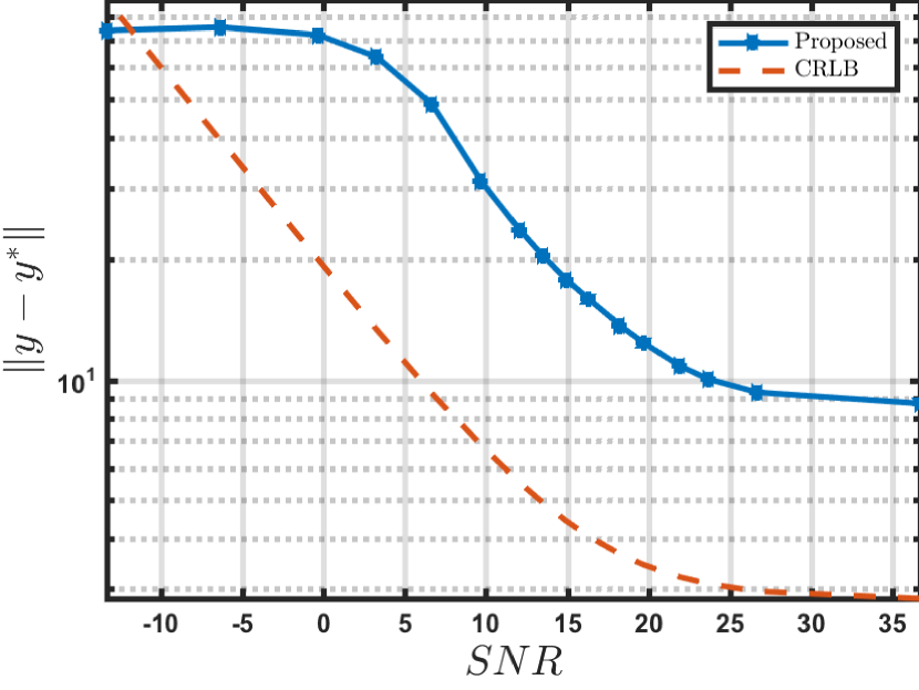
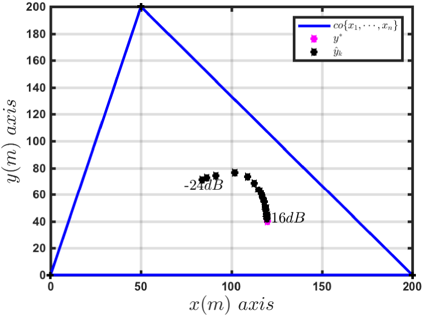
Fig. 2(a) shows the performance when N=2๐‘2N=2. The sensors are located at (0,0), (200,0) and (50,200), the source is at (120,40), cโ€‹oโ€‹{๐’™1,โ‹ฏ,๐’™N+1}๐‘๐‘œsubscript๐’™1โ‹ฏsubscript๐’™๐‘1co\{{\boldsymbol{x}_{1}},\cdots,{\boldsymbol{x}_{N+1}}\}. Fig. 2(b) presents the map of the average location estimate provided by our algorithm for various SNR values, as well as the actual source location.

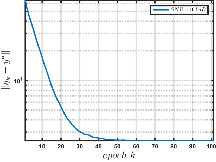
Fig. 3(a) is for gauging the convergence speed. For an SNR of 16.5dB, Fig. 3(a) plots the RMSE as a function of the iteration index k๐‘˜k. The RMSE at each value of k๐‘˜k is obtained by averaging over the 10000 random runs described above. The fast rate of convergence is self-evident.
Refer to caption
(a) RMSE against SNR.
Refer to caption
(b) Average source location
Figure 2: Simulations for N=2๐‘2N=2
Refer to caption
(a) RMSE vs eโ€‹pโ€‹oโ€‹cโ€‹hโ€‹k๐‘’๐‘๐‘œ๐‘โ„Ž๐‘˜epoch~{}k
Refer to caption
(b) RMSE vrs SNR, N=3๐‘3N=3
Figure 3: Average converging rate and โ„3superscriptโ„3\mathbb{R}^{3} simulations.

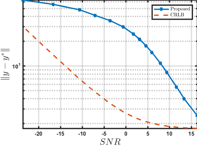
The 3-dimensional counterpart of Fig. 2(a) is depicted in Fig. 3(b). The sensors are at (0,0,0), (200,0,0), (0,200,0) and (0,0,100) and the source is at (10,20,10). The performance is depicted in figure 3(b).

It should be noted that in these simulations, except in low SNR regimes, the estimates do not leave cโ€‹oโ€‹{๐’™1,โ‹ฏ,๐’™N+1}๐‘๐‘œsubscript๐’™1โ‹ฏsubscript๐’™๐‘1co\{{\boldsymbol{x}_{1}},\cdots,{\boldsymbol{x}_{N+1}}\}. Even with low SNRs they leave the cโ€‹oโ€‹{๐’™1,โ‹ฏ,๐’™N+1}๐‘๐‘œsubscript๐’™1โ‹ฏsubscript๐’™๐‘1co\{{\boldsymbol{x}_{1}},\cdots,{\boldsymbol{x}_{N+1}}\} only about 10โˆ’3superscript10310^{-3}% of times. Further, the expectation of the signal at the sensors in the absence of noise are very small. For N=2๐‘2N=2 the received signals in the absence of noise are [1276,3192,490]Tsuperscript12763192490๐‘‡[1276,3192,490]^{T} whiles those for N=3๐‘3N=3 are [7054,372,449,3095]Tsuperscript70543724493095๐‘‡[7054,372,449,3095]^{T}. The simulations show the robustness of the algorithm.

VI Conclusion

A projection based gradient ascent localization of radioactive sources has been presented. It has been shown that if the source lies in the cโ€‹oโ€‹{๐’™1,โ‹ฏ,๐’™N+1}๐‘๐‘œsubscript๐’™1โ‹ฏsubscript๐’™๐‘1co\{{\boldsymbol{x}_{1}},\cdots,{\boldsymbol{x}_{N+1}}\}, then the maximum likelihood estimates has no false stationary points. The algorithm is proved to achieve global uniform asymptotic convergence in probability with simulations demonstrating robustness of algorithm.

References

  • [1] H.ย E. Baidoo-Williams, S.ย Dasgupta, R.ย Mudumbai, and E.ย Bai, โ€œOn the gradient descent localization of radioactive sources,โ€ IEEE Signal Processing Letters, vol.ย 20, no.ย 11, pp. 1046โ€“1049, 2013.
  • [2] H.ย E. Baidoo-Williams, โ€œNovel techniques for estimation and tracking of radioactive sources,โ€ Ph.D. dissertation, THE UNIVERSITY OF IOWA, 2014.
  • [3] P.ย Kump, E.-W. Bai, K.-S. Chan, and W.ย Eichinger, โ€œDetection of shielded radionuclides from weak and poorly resolved spectra using group positive rival,โ€ Radiation Measurements, vol.ย 48, pp. 18โ€“28, 2013.
  • [4] E.-w. Bai, A.ย Heifetz, P.ย Raptis, S.ย Dasgupta, and R.ย Mudumbai, โ€œMaximum likelihood localization of radioactive sources against a highly fluctuating background,โ€ IEEE Transactions on Nuclear Science, vol.ย 62, no.ย 6, pp. 3274โ€“3282, 2015.
  • [5] A.ย Gunatilaka, B.ย Ristic, and R.ย Gailis, โ€œOn localisation of a radiological point source,โ€ in Information, Decision and Control, 2007. IDCโ€™07.ย ย ย IEEE, 2007, pp. 236โ€“241.
  • [6] R.ย Vilim and R.ย Klann, โ€œRadtrac: A system for detecting, localizing, and tracking radioactive sources in real time,โ€ Nuclear technology, vol. 168, no.ย 1, pp. 61โ€“73, 2009.
  • [7] H.ย Khalil, โ€œInput-output stability,โ€ in Nonlinear Systems.ย ย ย Prentice Hall: Prentice Hall, 2002, ch.ย 5, pp. 195โ€“226.
  • [8] B.ย Fidan, S.ย Dasgupta, B.ย D. Anderson etย al., โ€œGuaranteeing practical convergence in algorithms for sensor and source localization,โ€ IEEE Transactions on Signal Processing, vol.ย 56, no.ย 9, pp. 4458โ€“4469, 2008.
  • [9] D.ย Blatt and A.ย O. Hero, โ€œEnergy-based sensor network source localization via projection onto convex sets,โ€ IEEE Transactions on Signal Processing, vol.ย 54, no.ย 9, pp. 3614โ€“3619, 2006.
  • [10] B.ย Anderson, R.ย R. Bitmead, C.ย R. Johnsonย Jr, P.ย V. Kokotovic, R.ย L. Kosut, I.ย M. Mareels, L.ย Praly, and B.ย D. Riedle, Stability of adaptive systems: Passivity and averaging analysis.ย ย ย MIT press, 1986.
  • [11] E.ย Yee, A.ย Gunatilaka, and B.ย Ristic, โ€œComparison of two approaches for detection and estimation of radioactive sources,โ€ ISRN Applied Mathematics, vol. 2011, 2011.
  • [12] B.ย Deb, โ€œIterative estimation of location and trajectory of radioactive sources with a networked system of detectors,โ€ IEEE Transactions on Nuclear Science, vol.ย 60, no.ย 2, pp. 1315โ€“1326, April 2013.
  • [13] N.ย S. Rao, M.ย Shankar, J.-C. Chin, D.ย K. Yau, C.ย Y. Ma, Y.ย Yang, J.ย C. Hou, X.ย Xu, and S.ย Sahni, โ€œLocalization under random measurements with application to radiation sources,โ€ in Information Fusion, 2008 11th International Conference on.ย ย ย IEEE, 2008, pp. 1โ€“8.
  • [14] J.ย W. Howse, L.ย O. Ticknor, and K.ย R. Muske, โ€œLeast squares estimation techniques for position tracking of radioactive sources,โ€ Automatica, vol.ย 37, no.ย 11, pp. 1727โ€“1737, 2001.
  • [15] A.ย Gunatilaka, B.ย Ristic, and R.ย Gailis, โ€œOn localisation of a radiological point source,โ€ in Information, Decision and Control, 2007. IDCโ€™07.ย ย ย IEEE, 2007, pp. 236โ€“241.
  • [16] M.ย R. Morelande and B.ย Ristic, โ€œRadiological source detection and localisation using bayesian techniques,โ€ IEEE Transactions on Signal Processing, vol.ย 57, no.ย 11, pp. 4220โ€“4231, 2009.
  • [17] A.ย H. Liu, J.ย J. Bunn, and K.ย M. Chandy, โ€œSensor networks for the detection and tracking of radiation and other threats in cities,โ€ in Information Processing in Sensor Networks (IPSN), 2011 10th International Conference on, April 2011, pp. 1โ€“12.