Phase estimation of phase shifts in two arms for an SU(1,1) interferometer with coherent and squeezed vacuum states

Abstract

We theoretically study the quantum Fisher information (QFI) of the SU(1,1) interferometer with phase shifts in two arms by coherent $\otimes$ squeezed vacuum state input, and give the comparison with the result of phase shift only in one arm. Different from the traditional Mach-Zehnder interferometer, the QFI of single-arm case for an SU(1,1) interferometer can be slightly higher or lower than that of two-arm case, which depends on the intensities of the two arms of the interferometer. For coherent $\otimes$ squeezed vacuum state input with a fixed mean photon number, the optimal sensitivity is achieved with a squeezed vacuum input in one mode and the vacuum input in the other.

I Introduction

Quantum enhanced metrology which has received a lot of attention in recent years is the use of quantum measurement techniques to obtain higher statistical precision than purely classical approaches Helstrom76 ; Holevo82 ; Caves81 ; Braunstein94 ; Braunstein96 ; Lee02 ; Giovannetti06 ; Zwierz10 ; Giovannetti04 ; Giovannetti11 ; Ou ; Abbott ; Hosten16 ; Xiang ; Zhang ; Wei . Mach-Zehnder interferometer (MZI) and its variants were used as a generic model to realize high precise estimation of phase. In order to achieve the ultimate lower bounds Zwierz ; Luca2015 , much work has been devoted to find the methods to improve the sensitivity of phase estimation, such as (1) using the nonclassical input states (quantum resources)-squeezed states Caves81 ; Xiao ; Grangier and NOON statesDowling08 ; NOON ; (2) using the new detection methods-homodyne detectionLi14 ; Hu and parity detection Anisimov ; Gerry2010 ; Chiruvelli ; Li2016 ; (3) using the nonlinear processes-amplitude amplification Yurke86 and phase magnification Hosten16 . Here we focus on the nonlinear amplitude amplification process to improve the sensitivity. In 1986, Yurke et al. Yurke86 introduced a new type of interferometer where two nonlinear beam splitters (NBSs) take the place of two linear beam splitters (BSs) in the traditional MZI. It is also called the SU(1,1) interferometer because it is described by the SU(1,1) group, as opposed to the traditional SU(2) MZI for BS. The detailed quantum statistics of the two-mode SU(1,1) interferometer was studied by Leonhardt Leonhardt . The SU(1,1) phase states were also studied theoretically in quantum measurements for phase-shift estimation Vourdas ; Sanders . Furthermore, the SU(1,1)-type interferometers have been reported by different groups using different systems in theory and experiment, such as all optical armsHudelist ; Lett ; Plick ; Marino , all atomic armsLinnemann16 ; Gabbrielli ; Gross , atom-light hybrid armsChenPRL15 ; Chen16 ; Yama ; Haine ; Szigeti ; Haine16 , light-circuit quantum electrodynamics system hybrid arms Barzanjeh , and all mechanical modes armsCheung . These SU(1,1)-type interferometers provide different methods for basic measurement.

At present, many researchers are focusing on how to measure the phase sensitivities, where several detection schemes have been presentedLi14 ; Li2016 ; Marino . In general, it is difficult to optimize all the detection schemes to obtain the optimal estimation protocol. However, the quantum Fisher information (QFI) Braunstein94 ; Braunstein96 characterizes the maximum amount of information that can be extracted from quantum experiments about an unknown parameter (e.g., phase shift $\phi$) using the best (and ideal) measurement device. Therefore, the lower bounds in quantum metrology can be obtained by using the method of the QFI. In recent years, many efforts were made to obtain the QFI of different measure systems Toth ; PezzBook ; Demkowicz ; Wang ; Jarzyna ; Monras ; Pinel ; Liu13 ; Gao ; Jiang ; Yan15 ; Safranek ; Sparaciari15 ; Ren16 ; Sparaciari ; Strobel ; Lu ; Hauke ; Liu17 . For the SU(1,1) interferometers with phase shift only in one arm, the QFI with coherent states input was studied by Sparaciari et al. Sparaciari15 ; Sparaciari , and the QFI with coherent $\otimes$ squeezed vacuum state input was presented by some of us Li2016 . Nevertheless in some measure schemes, the phase shifts in two arms are required to measure. For example, the phase sensitivity of phase shifts in two arms for the SU(1,1) interferometer with coherent states input was experimentally studied by Linnemann et al. Linnemann16 . Jarzyna et al. studied the QFIs of phase shifts in the two-arm case for a MZI, and presented the relation with the result of phase shift in the single-arm case Jarzyna . Since phase shift in the single arm is not simply equivalent to that phase shifts in two arms where one phase shift of them is $0$, the QFIs of phase shifts in two arms for an SU(1,1) interferometer are needed to research. In this paper, we study the QFI of SU(1,1) interferometer of phase shifts in two arms with two coherent states input and coherent $\otimes$ squeezed vacuum state input, and give the comparison with the result of phase shift only in one arm. These results should provide useful help to some phase measurement processes.

The remaining part of this paper is organized in the following way. In Section 2 we firstly give a brief review of the SU(1,1) interferometer, then derive the QFI of phase shifts in two arms for an SU(1,1) interferometer. In Section 3 the phase sensitivities of SU(1,1) interferometer obtained from the quantum Cramér-Rao bound (QCRB) Helstrom76 ; Holevo82 are discussed, and the results of phase shifts in different arms are compared. The conclusions are summarized in Section 4.

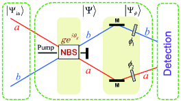
Figure 1: Schematic diagram of the parameter estimation process based on the SU(1,1) interferometer. $g$ and $\theta_{g}$ describe the strength and phase in the first NBS process, respectively. $a$ and $b$ denote two light modes in the interferometer. In the Schrödinger picture the initial state $|\Psi_{\mathrm{in}}\rangle$ injecting into a NBS results in the output $|\Psi\rangle$, and the state is transformed as $|\Psi_{\phi}\rangle$ after phase shifts. NBS: nonlinear beam splitter; $\phi_{1}$, $\phi_{2}$: phase shifts; $\mathrm{M}$: mirrors.

II The QFI of phase shifts in two arms for an SU(1,1) interferometer

Because the QFI $\mathcal{F}$ is the intrinsic information in the quantum state and is not related to actual measurement procedure as shown in Fig. 1. It establishes the best precision that can be attained with a given quantum probe Braunstein94 ; Braunstein96 . In this section, we study the QFIs of SU(1,1) interferometer of phase shifts in two arms, and compare them with the results of phase shift only in one arm.

II.1 NBS and phase shifts

In an SU(1,1) interferometer, the NBSs take the place of the BSs in the traditional MZI shown in Fig. 1. Firstly, we theoretically describe the NBS briefly, which can be completed by the optical parameter amplifier (OPA) or four-wave mixing (FWM) process. The annihilation operators of the two modes $a$, $b$ and the pump field are $\hat{a}$, $\hat{b}$, and $\hat{c}$, respectively. The interaction Hamiltonian for NBS is of the form

$$\hat{H}=i\hbar\eta^{\ast}\hat{a}\hat{c}^{\dagger}\hat{b}\hat{c}^{\dagger}-i\hbar\eta\hat{a}^{\dagger}\hat{c}\hat{b}^{\dagger}\hat{c}.$$ (1)

Because the pump field is very strong and the intensity of the pump field is not significantly changed in the mixing process. Then the initial and final states of the pump field are the same as the coherent state $|\alpha_{\mathrm{pump}}\rangle$. Under the undepleted pump approximation, the Hamiltonian is written as

$$\hat{H}=i\hbar\eta^{\ast}\alpha_{\mathrm{pump}}^{\ast 2}\hat{a}\hat{b}-i\hbar\eta\alpha_{\mathrm{pump}}^{2}\hat{a}^{\dagger}\hat{b}^{\dagger}.$$ (2)

The corresponding time-evolution operator is $\hat{U}(t)=e^{-i\hat{H}t/\hbar}=\exp(-\xi\hat{a}^{\dagger}\hat{b}^{\dagger}+\xi^{\ast}\hat{a}\hat{b})$, where $\xi=\eta\alpha_{\mathrm{pump}}^{2}t=ge^{i\theta_{g}}$ is the two-mode squeezing parameter. In the Schrödinger picture the initial state $|\Psi_{\mathrm{in}}\rangle$ injecting into a NBS results in the output $|\Psi\rangle=\hat{U}(t)|\Psi_{\mathrm{in}}\rangle$, where the transformation of the annihilation operators is

$$\left(\begin{array}[]{c}\hat{a}^{\prime}\\ \hat{b}^{{}^{\dagger}\prime}\end{array}\right)=\left(\begin{array}[]{cc}\cosh g&-e^{i\theta_{g}}\sinh g\\ -e^{-i\theta_{g}}\sinh g&\cosh g\end{array}\right)\left(\begin{array}[]{c}\hat{a}\\ \hat{b}^{{}^{\dagger}}\end{array}\right).$$ (3)

Secondly, we describe the phase shifts process. Different from the BS, the NBS involves three light fields where the pump field is classical and with a classical reference phase. The uncertainty of classical pump field $1/\sqrt{|\alpha_{\mathrm{pump}}|^{2}}$ is very small and the phase uncertainties are from the modes $a$ and $b$. After the first NBS, as shown in Fig. 1, the two beams sustain phase shifts, i.e., the mode $a$ and mode $b$ undergo the phase shifts of $\phi_{1}$ and $\phi_{2}$, respectively. Then we may write

$$\exp\left(i\phi_{1}\hat{a}^{\dagger}\hat{a}\right)\exp\left(i\phi_{2}\hat{b}^{\dagger}\hat{b}\right)$$ (4)

$$= \exp\left[i\frac{\phi_{1}+\phi_{2}}{2}(\hat{a}^{\dagger}\hat{a}+\hat{b}^{\dagger}\hat{b})\right]\exp\left[i\frac{\phi_{1}-\phi_{2}}{2}(\hat{a}^{\dagger}\hat{a}-\hat{b}^{\dagger}\hat{b})\right]$$

$$= \exp\left[i\frac{\phi}{\hbar}\hat{K}_{z}-i\frac{\phi}{2}\right]\exp\left[i\frac{(\phi_{1}-\phi_{2})}{\hbar}\hat{J}_{z}\right],$$

where $\phi=\phi_{1}+\phi_{2}$, $\hat{K}_{z}=\hbar(\hat{a}^{\dagger}\hat{a}+\hat{b}^{\dagger}\hat{b}+1)/2$, and $\hat{J}_{z}=\hbar(\hat{a}^{\dagger}\hat{a}-\hat{b}^{\dagger}\hat{b})/2$. In the Schrödinger picture the transformation of the incoming state vector $\left|\Psi\right\rangle$ is given as following

$$|\Psi_{\phi}\rangle=e^{-i\phi/2}e^{i(\phi_{1}-\phi_{2})/\hbar\hat{J}_{z}}e^{-i\phi/\hbar\hat{K}_{z}}\left|\Psi\right\rangle.$$ (5)

$\hat{J}_{z}$ is an invariant for the four-wave mixing process. The operator $e^{i(\phi_{1}-\phi_{2})/\hbar\hat{J}_{z}}$ gives rise to phase factors which does not contribute to the expectation values of number operators.

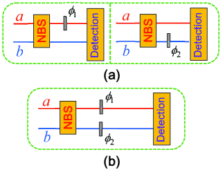
Figure 2: Different phase delay ways of the interferometer: (a) Phase shift in the single arm is divided into single upper arm and single lower arm due to the intensities of the two arms are not equal. (b) Phase shifts in the two arms.

II.2 QFI

The QFI is the intrinsic information in the quantum state and it is not related to actual measurement procedure, and is at least as great as the classical Fisher information for the optimal observable. The QFI $\mathcal{F}$ is defined as Braunstein94 ; Braunstein96

$$\mathcal{F}=\mathrm{Tr}[\rho(\phi)L_{\phi}^{2}],$$ (6)

where the Hermitian operator $L_{\phi}$, called symmetric logarithmic derivative, is defined as the solution of the equation $\partial_{\phi}\rho(\phi)=[\rho(\phi)L_{\phi}+L_{\phi}\rho(\phi)]/2$. In terms of the complete basis $\{|k\rangle\}$ such that $\rho(\phi)=\sum_{k}p_{k}|k\rangle\langle k|$ with $p_{k}\geq 0$ and $\sum_{k}p_{k}=1$, the QFI can be written as Braunstein94 ; Braunstein96 ; Toth ; PezzBook ; Demkowicz

$$\mathcal{F}=\sum_{k,k^{\prime}}\frac{2}{p_{k}+p_{k^{\prime}}}\left|\langle k|\partial_{\phi}\rho(\phi)|k^{\prime}\rangle\right|^{2}.$$ (7)

Under the condition of lossless, for a pure state the QFI is reduced to Jarzyna ; PezzBook

$$\mathcal{F}=4\left(\langle\Psi_{\phi}^{\prime}|\Psi_{\phi}^{\prime}\rangle-\left|\langle\Psi_{\phi}^{\prime}|\Psi_{\phi}\rangle\right|^{2}\right),$$ (8)

where $|\Psi_{\phi}^{\prime}\rangle=\partial|\Psi_{\phi}\rangle/\partial\phi$. In general, the QFI bounds depend on the ways that the interferometer phase delay is modeled: (I) phase shift only in the single arm, and (II) phase shifts distributed in two arms, which is shown in Fig. 2(a) and (b), respectively. Hereafter, we use the single-arm case (S) and two-arm case (T) to denote them.

Now, we give the QFIs with different input states under the condition of phase shifts in two arms. From Eq. (5), $|\Psi_{\phi}\rangle$ is the state vector just before the detection process of the SU(1,1) interferometer and $|\Psi_{\phi}^{\prime}\rangle=-i(1/2+\hat{K}_{z}/\hbar)\left|\Psi_{\phi}\right\rangle$. Then from Eq. (8) the QFI can be worked out:

$$\mathcal{F}=\frac{4}{\hbar^{2}}\Delta^{2}\hat{K}_{z},$$ (9)

where $\Delta^{2}\hat{K}_{z}=\langle\Psi|\hat{K}_{z}^{2}|\Psi\rangle-\langle\Psi|\hat{K}_{z}|\Psi\rangle^{2}$. Using the transforms of Eqs. (3) and (5) and with two coherent states $|\alpha\rangle\otimes|\beta\rangle$ ($j=\left|j\right|e^{i\theta_{j}}$, $N_{j}=\left|j\right|^{2}$, $j=\alpha$, $\beta$) input case, for the SU(1,1) interferometer we have

$$\mathcal{F}_{\mathrm{coh\&coh}}^{\mathrm{T}} = (N_{\alpha}+N_{\beta})\cosh(4g)+\sinh^{2}(2g)$$

$$+2\sinh(4g)\sqrt{N_{\alpha}N_{\beta}}\cos(\theta_{\alpha}+\theta_{\beta}-\theta_{g}-\pi).$$

When $\theta_{\alpha}+\theta_{\beta}-\theta_{g}=\pi$, the maximal QFI $\mathcal{F}_{\mathrm{coh\&coh}}^{\mathrm{T}}$ is reduced to

$$\mathcal{F}_{\mathrm{coh\&coh}}^{\mathrm{T}}=(N_{\alpha}+N_{\beta})\cosh(4g)+\sinh^{2}(2g)+2\sinh(4g)\sqrt{N_{\alpha}N_{\beta}}.$$ (11)

When $N_{\alpha}=N_{\beta}=0$ (vacuum input) and $N_{\alpha}\neq 0$, $N_{\beta}=0$ (one coherent state input), from Eq. (11) the corresponding QFIs are given by $\mathcal{F}_{\mathrm{vac}}^{\mathrm{T}}=\sinh^{2}(2g)$ and $\mathcal{F}_{\mathrm{coh\&vac}}^{\mathrm{T}}=N_{\alpha}\cosh 4g+\sinh^{2}(2g)$, respectively.

Next, we consider a coherent light combined with a squeezed vacuum light as the input $|\psi_{in}\rangle=|\alpha\rangle_{a}\otimes|0,\varsigma\rangle_{b}$ ($\alpha=\left|\alpha\right|e^{i\theta_{\alpha}}$, $N_{\alpha}=\left|\alpha\right|^{2}$, and $|0,\varsigma\rangle_{b}=\hat{S}_{b}(r)|0\rangle_{b}$ is the single-mode squeezed vacuum state in the $b$-mode where $\hat{S}_{b}(r)=\exp[(\varsigma^{\ast}\hat{b}^{2}-\varsigma\hat{b}^{{\dagger}2})/2]$ with $\varsigma=r\exp(i\theta_{\varsigma})$ is the single-mode squeezing parameter), and the QFI can be worked out:

$$\mathcal{F}_{\mathrm{coh\&squ}}^{\mathrm{T}} = \cosh^{2}(2g)\left[\frac{1}{2}\sinh^{2}(2r)+N_{\alpha}\right]$$ (13)

$$+\sinh^{2}(2g)[N_{\alpha}(\cosh 2r-\sinh 2r\cos\Phi)+\cosh^{2}r],$$

where $\Phi=\theta_{\varsigma}+2\theta_{\alpha}-2\theta_{g}$. When $\Phi=\pi$, the maximal QFI $\mathcal{F}_{\mathrm{coh\&squ}}^{\mathrm{T}}$ is given by

$$\mathcal{F}_{\mathrm{coh\&squ}}^{\mathrm{T}} = \cosh^{2}(2g)\left[\frac{1}{2}\sinh^{2}(2r)+N_{\alpha}\right]$$ (14)

$$+\sinh^{2}(2g)[N_{\alpha}e^{2r}+\cosh^{2}r].$$

When $r=0$, $\mathcal{F}_{\mathrm{coh\&squ}}^{\mathrm{T}}$ is also reduced to $\mathcal{F}_{\mathrm{coh\&vac}}^{\mathrm{T}}$, which agrees with the above result. This input state was also used to improve the phase-shift measurement sensitivity in the SU(1,1) interferometer but only with the method of the error propagation in Ref.  Li14 .

So far, we have given the QFI of SU(1,1) interferometer where the phase shifts in the two arms, and they as well as the QFIs with phase shift in the one arm case are summarized in the Table I. From this Table, the QFIs of phase shift in upper arm and in lower arm are also slightly different because the intensities in two arms of the interferometer are unbalanced. The QFI of single-arm case for an SU(1,1) interferometer can be slightly higher or lower than that of double arms case, which depends on the intensities of the two arms of the interferometer. Different from the SU(1,1) interferometer, the QFIs of the phase shifts in single upper arm and in single lower arm are the same due to the intensity balance of the two arms for the MZI Jarzyna .

III QCRB

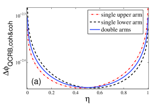
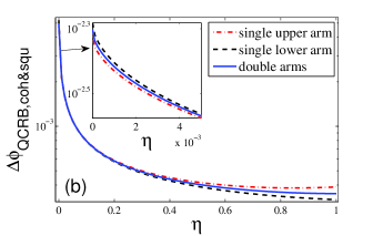
Figure 3: The QCRB versus the $\eta$ for (a) two coherent states input; (b) coherent $\otimes$ squeezed state input. The inset in figure (b) shows a zoom of the graph for small values of $\eta$. Parameters: $N_{\mathrm{in}}=200$, and $g=1.5$.

Whatever the measurement chosen, the QCRB can give the lower bound for the phase measurement Braunstein94 ; Braunstein96 ; Toth ; PezzBook ; Demkowicz

$$\Delta\phi_{\mathrm{QCRB}}=\frac{1}{\sqrt{\mathcal{F}}}.$$ (15)

To describe the effect on the QCRB from the unbalanced input state, we introduce a parameter $\eta$ which is defined by Hu

$$\eta=\frac{\mathrm{mean~{}photon~{}number~{}of~{}}b\mathrm{~{}mode}}{\mathrm{total~{}mean~{}photon~{}number~{}of~{}input}}.$$ (16)

For the two coherent states input, $\eta$ is equal to $N_{\beta}/N_{\mathrm{in}}$ ($N_{\mathrm{in}}=N_{\alpha}+N_{\beta}$), and the optimal phase sensitivities $\Delta\phi_{\mathrm{QCRB}}$ as a function of $\eta$ are shown in Fig. 3(a). When $\eta$ is small, the $\Delta\phi_{\mathrm{QCRB}}$ from the single upper arm case is the best. But when $\eta$ is large, the $\Delta\phi_{\mathrm{QCRB}}$ from the single lower arm case is the best, and the $\Delta\phi_{\mathrm{QCRB}}$ from the two-arm case is always an intermediate value. For a given fixed $N_{\mathrm{in}}$, and the two coherent states input case, the optimal value $\eta$ is $0.5$. That is for the two coherent states input the optimal input state is $|\sqrt{N_{\mathrm{in}}/2}e^{i\theta_{\alpha}}\rangle\otimes|-\sqrt{N_{\mathrm{in}}/2}e^{-i\theta_{\alpha}}e^{i\theta_{g}}\rangle$, and the corresponding optimal QFI is $\mathcal{F}_{\mathrm{coh\&coh}}^{\mathrm{T,opt}}=N_{\mathrm{in}}e^{4g}+\sinh^{2}(2g)$. The optimal QFI $\mathcal{F}_{\mathrm{coh\&coh}}^{\mathrm{T,opt}}$ as a function of the total input mean photon number $N_{\mathrm{in}}$ is shown in Fig. 4 (the blue dot-dashed line).

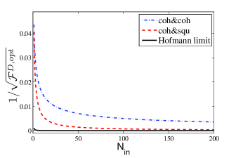
Figure 4: The optimal QFIs versus the total input mean photon number $N_{\mathrm{in}}$. The dot-dashed line and the dashed line are the two coherent states input and coherent $\otimes$ squeezed state input, respectively. The solid line is the Hofmann limit with coherent $\otimes$ squeezed state input. $g=1.5$.

For coherent $\otimes$ squeezed vacuum state input, $\eta$ is equal to $\sinh^{2}r/N_{\mathrm{in}}$ ($N_{\mathrm{in}}=N_{\alpha}+\sinh^{2}r$), where the parameter $\eta$ can be used to label the squeezing fraction of the mean photon number. When $\eta=0$ or $\eta=1$, the input state is only a coherent state $|\alpha\rangle_{a}$ or only a squeezed vacuum state $|0,\zeta\rangle_{b}$. When $0<\eta<1$, the input state is a coherent $\otimes$ squeezed vacuum state. For coherent $\otimes$ squeezed vacuum state input case, only the squeezed vacuum light as input and without the coherent state, the phase sensitivity is the highest shown in Fig. 3(b). That is the optimal input state is $|0\rangle\otimes|0,\zeta\rangle$, and the corresponding optimal QFI is $\mathcal{F}_{\mathrm{coh\&squ}}^{\mathrm{T,opt}}=(1+N_{\mathrm{in}})[2N_{\mathrm{in}}\cosh^{2}(2g)+\sinh^{2}(2g)]$, which is different from the commonly used optimal input state with $\left|\alpha\right|^{2}\simeq\sinh^{2}(r)\simeq N_{\mathrm{in}}/2$ in MZI Pezz08 ; Lang13 ; Liu13 . The reason is the number fluctuations and Pasquale et al. Pasquale have given the same result for generic two-mode interferometric setup recently. The optimal QFI $\mathcal{F}_{\mathrm{coh\&squ}}^{\mathrm{T,opt}}$ as a function of $N_{\mathrm{in}}$ is shown in Fig. 4 (the red dashed line). For a fixed mean photon number (with number fluctuations), Hofmann suggested the form of Heisenberg limit is $1/\langle\hat{N}^{2}\rangle^{1/2}$, which indicates averaging over the squared photon numbers hofmann . In our proposal $\langle\hat{N}\rangle$ is defined as $\langle\Psi|(\hat{n}_{a}+\hat{n}_{b})|\Psi\rangle$. In Fig. 4 the black solid line is the Hofman limit for coherent $\otimes$ squeezed vacuum state input under the optimal condition.

For the lossy interferometers, the pure states evolve into the mixed states and the QFI will be reduced. However, the QFI of pure state puts an upper bound on that of mixed state. Here, we focus on the maximal QFI of the SU(1,1) interferometer, then we ignore the losses in the interferometer.

IV Conclusion

In conclusion, the analytical expressions of QFI for an SU(1,1) interferometer with two coherent states and coherent $\otimes$ squeezed vacuum state inputs have been derived. For single-arm case, the QCRBs of phase shift in upper arm and in lower arm are slightly different because the intensities in two interferometric arms are asymmetric. The phase sensitivities of phase shifts between the single-arm case and two-arm case are also compared. The QCRB of single-arm case can be slightly higher or lower than that of two-arm case, which depends on the intensities of the two arms of the interferometer. For coherent state $\otimes$ squeezed vacuum state input with a definite input number of photons, the optimal condition to obtain the highest phase sensitivity is a squeezed vacuum in one mode and the vacuum state in the other mode.

Table 1: The maximal QFIs of the SU(1,1) interferometer for different phase delay ways with different input states

	single arm $\mathcal{F}^{\mathrm{S}}$		phase shifts in
input states	phase shift in upper arm	phase shift in lower arm	two arms $\mathcal{F}^{\mathrm{T}}$
two coherent states	$(N_{\alpha}+N_{\beta})\cosh 4g+\sinh^{2}(2g)$	$(N_{\alpha}+N_{\beta})\cosh 4g+\sinh^{2}(2g)$	$(N_{\alpha}+N_{\beta})\cosh 4g$
$|\alpha\rangle_{a}\otimes|\beta\rangle_{b}$	$+2\sqrt{N_{\alpha}N_{\beta}}\sinh 4g+N_{\alpha}+N_{\beta}$	$+2\sqrt{N_{\alpha}N_{\beta}}\sinh 4g+N_{\alpha}+N_{\beta}$	$\ +\sinh^{2}(2g)$
	$+2(N_{\alpha}-N_{\beta})\cosh 2g$a	$-2(N_{\alpha}-N_{\beta})\cosh 2g$	$+2\sqrt{N_{\alpha}N_{\beta}}\sinh 4g$
coherent $\otimes$ squee	$\cosh^{2}(2g)[\sinh^{2}(2r)/2+N_{\alpha}]$	$\cosh^{2}(2g)[\sinh^{2}(2r)/2+N_{\alpha}]$	$\cosh^{2}(2g)[N_{\alpha}$
-zed vacuum states	$+\sinh^{2}(2g)[N_{\alpha}e^{2r}+\cosh^{2}r]$	$+\sinh^{2}(2g)[N_{\alpha}e^{2r}+\cosh^{2}r]$	$+\sinh^{2}(2r)/2]$
$|\alpha\rangle_{a}\otimes|\varsigma,0\rangle_{b}$	$+N_{\alpha}(1+2\cosh 2g)$	$+N_{\alpha}(1-2\cosh 2g)$	$+\sinh^{2}(2g)[N_{\alpha}e^{2r}$
$\left(\varsigma=r\exp(i\theta_{\varsigma})\right)$	$-\frac{1}{4}(\cosh 4r-1)(2\cosh 2g-1)^{\mathrm{b}}$	$+\frac{1}{4}(\cosh 4r-1)(2\cosh 2g+1)^{\mathrm{b}}$	$+\cosh^{2}r]$
aRef.  Sparaciari .
bRef.  Li2016 .

References

- (1) Helstrom C W 1976 Quantum Detection andEstimation Theory (Academic, New York)
- (2) Holevo A S, 1982 Probabilistic and Statistical Aspect of Quantum Theory (North-Holland, Amsterdam).
- (3) Caves C M 1981 Phys. Rev. D 23, 1693
- (4) Braunstein S L and Caves C M 1994 Phys. Rev. Lett. 72, 3439
- (5) Braunstein S L, Caves C M, and Milburn G J 1996 Ann. Phys. 247, 135
- (6) Lee H, Kok P, and Dowling J P 2002 J. Mod. Opt. 49, 2325
- (7) Giovannetti V , Lloyd S , and Maccone L 2006 Phys. Rev. Lett. 96, 010401
- (8) Zwierz M, Pérez-Delgado C A, and Kok P 2010 Phys. Rev. Lett. 105, 180402
- (9) Giovannetti V, Lloyd S, and Maccone L 2004 Science 306, 1330
- (10) Giovannetti V, Lloyd S, and Maccone L 2011 Nature photonics 5, 222
- (11) Ou Z Y 2012 Phys.Rev. A 85, 023815
- (12) Abbott B P et al. (LIGO Scientific Collaboration and Virgo Collaboration) 2016 Phys. Rev. Lett. 116, 061102
- (13) Hosten O, Krishnakumar R, Engelsen N J, Kasevich M A 2016 Science 352, 1552
- (14) Xiang G Y and Guo G C 2013 Chin. Phys. B 22, 110601
- (15) Zhang L J and Xiao M 2013 Chin. Phys. B 22, 110310
- (16) Wei C P, Hu X Y, Yu Y F, and Zhang Z M 2016 Chin. Phys. B 25, 040601
- (17) Zwierz M, Pérez-Delgado C A, and Kok P 2012 Phys. Rev. A 85, 042112
- (18) Pezzè L, Hyllus P, and Smerzi A 2015 Phys. Rev. A 91, 032103.
- (19) Xiao M, Wu L A, and Kimble H J 1987 Phys. Rev. Lett. 59, 278
- (20) Grangier P, Slusher R E, Yurke B, and LaPorta A 1987 Phys. Rev. Lett. 59, 2153
- (21) Dowling J P 2008 Contemporary Physics 49, 125
- (22) Boto A N, Kok P, Abrams D S, Braunstein S L, Williams C P, and Dowling J P 2000 Phys. Rev. Lett. 85, 2733
- (23) Li D, Yuan C H, Ou Z Y, and Zhang W 2014 New J. Phys. 16, 073020
- (24) Hu X Y, Wei C P, Yu Y F, and Zhang Z M 2016 Front. Phys. 11 114203
- (25) Anisimov P M, Raterman G M, Chiruvelli A, Plick W N , Huver S D, Lee H, and Dowling J P 2010 Phys. Rev. Lett. 104, 103602
- (26) Gerry C C and Mimih J 2010 Contemporary Physics 51, 497
- (27) Chiruvelli A and Lee H 2011 Journal of Modern Opt. 58, 945
- (28) Li D, Gard Bryan T, Gao Y, Yuan C-H, Zhang W, Lee H, and Dowling J P 2016 Phys. Rev. A 94, 063840
- (29) Yurke B, McCall S L, and Klauder J R Phys. Rev. A 33, 4033
- (30) Leonhardt U 1994 Phys. Rev. A 49, 1231
- (31) Vourdas A 1990 Phys. Rev. A 41, 1653
- (32) Sanders B C, Milburn G J, and Zhang Z 1997 J. Mod. Opt. 44, 1309
- (33) Hudelist F, Kong J, Liu C, Jing J, Ou Z Y, and Zhang W 2014 Nat. Commun. 5, 3049
- (34) Anderson B E, Gupta P, Schmittberger B L, Horrom T, Hermann-Avigliano C, Jones K M, and Lett Paul D arXiv: 1610.06891v1 [quant-ph]
- (35) Plick W N, Dowling J P, and Agarwal G. S 2010 New J. Phys. 12, 083014
- (36) Marino A M, Corzo Trejo N V, and Lett P D 2012 Phys. Rev. A 86, 023844
- (37) Linnemann D, Strobel H, Muessel W, Schulz J, Lewis-Swan R J, Kheruntsyan K V, and Oberthaler M K 2016 Phys. Rev. Lett. 117, 013001
- (38) Gabbrielli M, Pezzè L, and Smerzi A 2015 Phys. Rev. Lett. 115, 163002
- (39) Gross C, Zibold T, Nicklas E, Estève J, and Oberthaler M K 2010 Nature 464, 1165
- (40) Chen B, Qiu C, Chen S, Guo J, Chen L Q, Ou Z Y, and Zhang W 2015 Phys. Rev. Lett. 115, 043602
- (41) Chen Z D, Yuan C-H, Ma H M, Li D, Chen L Q, Ou Z Y, and Zhang W 2016 Opt. Express 24, 17766
- (42) Jacobson J, Björk G, and Yamamoto Y 1995 Appl. Phys. B 60, 187
- (43) Haine S A 2014 Phys. Rev. Lett. 112,120405
- (44) Szigeti S S, Tonekaboni B, Lau W Y S, Hood S N, and Haine S A 2014 Phys. Rev. A 90, 063630
- (45) Haine S A, and Lau W Y S 2016 Phys. Rev. A 93, 023607
- (46) Barzanjeh Sh, DiVincenzo D P, and Terhal B M 2014 Phys. Rev. B 90, 134515 .
- (47) Cheung H F H, Patil Y S, Chang L, Chakram S and Vengalattore M arXiv:1601.02324v1 [quant-ph]
- (48) Toth G and Apellaniz I 2014 J. Phys. A 47, 424006
- (49) Pezzè L and Smerzi A 2014 in Proceedings of the International School of Physics “Enrico Fermi ”, Course CLXXXVIII “Atom Interferometry”edited by G. Tino and M. Kasevich (Società Italiana di Fisica and IOS: Bologna), p. 691
- (50) Demkowicz-Dobrzanski R., Jarzyna M., Kolodynski J 2015 Progress in Optics 60, 345
- (51) Wang X-B, Hiroshima T, Tomita A, Hayashi M 2007 Physics Reports 448, 1
- (52) Jarzyna M and Demkowicz-Dorbrzanski R 2012 Phys. Rev. A 85, 011801(R)
- (53) Monras A 2013 arXiv:1303.3682v1 [quant-ph]
- (54) Pinel O, Jian P, Treps N, Fabre C, and Braun D 2013 Phys. Rev. A 88, 040102(R)
- (55) Liu Jing, Jing Xiaoxing, and Wang Xiaoguang 2013 Phys.Rev. A 88, 042316
- (56) Gao Y and Lee H 2014 Eur. Phys. J. D 68, 347
- (57) Jiang Z 2014 Phys. Rev. A 89, 032128
- (58) Li Yan-Ling, Xiao Xing, and Yao Yao 2015 Phys. Rev. A 91, 052105
- (59) Safranek D, Lee A R, and Fuentes I 2015 New J. Phys. 17, 073016
- (60) Sparaciari C, Olivares S, and Paris M G A 2015 J. Opt. Soc. Am. B 32, 1354
- (61) Ren Yu-Kun, Tang La-Mei, and Zeng Hao-Sheng 2016 Quantum Inf. Process15, 5011
- (62) Sparaciari C, Olivares S, and Paris M G A 2016 Phys. Rev. A 93, 023810
- (63) Strobel H, Muessel W, Linnemann D, Zibold T Hume D B, Pezze L, Smerzi A, and Oberthaler M K, 2014 Science 345, 424
- (64) Lu X M, Yu S, and Oh C H 2015 Nat. Commun. 6, 7282
- (65) Hauke P, Heyl M, Tagliacozzo L, and Zoller P 2016 Nat. Phys. 12, 778
- (66) Liu P, Wang P, Yang W, Jin G R, and Sun C P 2017 Phys. Rev. A 95, 023824
- (67) Pezzè L and Smerzi A 2008 Phys. Rev. Lett. 100, 073601
- (68) Lang M D and Caves C M 2013 Phys. Rev. Lett. 111, 173601
- (69) Pasquale A D, Facchi P, Florio G, Giovannetti V, Matsuoka K, and Yuasa K 2015 Phys. Rev. A 92, 042115
- (70) Hofmann H F 2015 Phys. Rev. A 79, 033822