An interacting quark-diquark model. Strange and nonstrange baryon spectroscopy and other observables

Abstract

We describe the relativistic interacting quark-diquark model formalism and its application to the calculation of strange and nonstrange baryon spectra. The results are compared to the existing experimental data. We also discuss the application of the model to the calculation of other baryon observables, like baryon magnetic moments, open-flavor strong decays and baryon masses with self-energy corrections.

I Introduction

The diquark concept has been used in a large number of studies, ranging from one-gluon exchange to lattice QCD calculations. For example, see Refs. Jakob:1997 ; Jaffe:2003 ; Wilczek:2004im ; Jaffe:2004ph ; Santopinto:2004hw ; Selem:2006nd .

Recently, an interacting quark-diquark model has been introduced by Santopinto in Ref. Santopinto:2004hw . This is a nonrelativistic potential model, where baryons are described as two-body quark-diquark bound states and the relative motion between the quark and diquark constituents in terms of a relative coordinate $\vec{r}$. The Hamiltonian contains a Coulomb-like plus linear confining interaction and an exchange one, depending on the spins and isospins of the quark and the diquark. In this article, we will discuss the main features of the interacting quark-diquark model, as relativistically reformulated in Refs. Ferretti:2011zz ; qD2014b ; qD2014a ; charmed-baryons within the point form formalism Klink:1998zz .

Finally, we will summarize our results for the strange and nonstrange baryon spectra Santopinto:2004hw ; Ferretti:2011zz ; qD2014b ; qD2014a and baryon magnetic moments in the quark-diquark model qD2014a . We will also briefly discuss the formalism to calculate other baryon observables in the quark-diquark model, including open-flavor strong decays and baryon masses with self-energy corrections.

II An interacting quark-diquark model

In quark-diquark models, baryons are assumed to be composed of a constituent quark and a constituent diquark GellMann:1964nj ; Ida:1966ev ; lich . Up to an energy of 2 GeV, the diquark can be described as two correlated quarks with no internal spatial excitations Santopinto:2004hw ; Ferretti:2011zz . Then, its color-spin-flavor wave function must be antisymmetric. Moreover, as we consider only light baryons, made up of $u$, $d$, $s$ quarks, the internal group is restricted to SU_sf(6). If we denote spin by its value, flavor and color by the dimension of the representation, the quark has spin $s_{2}=\frac{1}{2}$, flavor $F_{2}={\bf{3}}$, and color $C_{2}={\bf{3}}$. The diquark must transform as ${\bf{\overline{3}}}$ under SU_c(3), hadrons being color singlets. Then, one only has the symmetric SU_sf(6) representation $\mbox{{\boldmath{$21$}}}_{\rm sf}$(S), containing $s_{1}=0$, $F_{1}={\bf{\overline{3}}}$ (the scalar diquark) and $s_{1}=1$, $F_{1}={\bf{6}}$ (the axial-vector diquark) Wilczek:2004im ; Jaffe:2004ph .

II.1 Model Hamiltonian and calculation of the strange and nonstrange baryon spectra

The Hamiltonian of the model is Ferretti:2011zz

$$\begin{array}[]{rcl}M&=&E_{0}+\sqrt{\vec{q}\hskip 2.27626pt^{2}+m_{1}^{2}}+\sqrt{\vec{q}\hskip 2.27626pt^{2}+m_{2}^{2}}+M_{\rm dir}(r)+M_{\rm ex}(r)\end{array}\mbox{ }.$$ (1)

Here, $E_{0}$ is a constant, $M_{\rm dir}(r)$ and $M_{\rm ex}(r)$ are the direct and exchange quark-diquark interactions, respectively, $m_{1}$ and $m_{2}$ the diquark and quark masses. The direct term,

$$M_{\rm dir}(r)=-\frac{\tau}{r}\left(1-e^{-\mu r}\right)+\beta r~{}~{},$$ (2)

is the sum of a Coulomb-like interaction with a cut off plus a linear confinement term. The exchange interaction is given by Santopinto:2004hw ; Ferretti:2011zz ,

$$\begin{array}[]{rcl}M_{\rm ex}(r)&=&\left(-1\right)^{L+1}\mbox{ }e^{-\sigma r}\left[A_{\rm S}\mbox{ }\vec{s}_{1}\cdot\vec{s}_{2}+A_{\rm I}\mbox{ }\vec{t}_{1}\cdot\vec{t}_{2}+A_{\rm SI}\mbox{ }\vec{s}_{1}\cdot\vec{s}_{2}\mbox{ }\vec{t}_{1}\cdot\vec{t}_{2}\right]\end{array}\mbox{ },$$ (3)

where $\vec{s}$ and $\vec{t}$ are the spin and isospin operators. To calculate the strange baryon spectrum, Eq. (3) has to be generalized in the form of a Gürsey-Radicati interaction qD2014b ; Gursey:1992dc ,

$$\begin{array}[]{rcl}M_{\rm ex}(r)&=&\left(-1\right)^{L+1}\mbox{ }e^{-\sigma r}\left[A_{\rm S}\mbox{ }\vec{s}_{1}\cdot\vec{s}_{2}+A_{\rm F}\mbox{ }\vec{\lambda}_{1}^{\rm f}\cdot\vec{\lambda}_{2}^{\rm f}\mbox{ }+A_{\rm I}\mbox{ }\vec{t}_{1}\cdot\vec{t}_{2}\right]\end{array}\mbox{ },$$ (4)

where $\vec{\lambda}^{\rm f}$ are SU_f(3) Gell-Mann matrices. In the nonstrange sector, we also have a contact interaction Santopinto:2004hw ; Ferretti:2011zz ,

$$\begin{array}[]{rcl}M_{\rm cont}(r)&=&\left(\frac{m_{1}m_{2}}{E_{1}E_{2}}\right)^{1/2+\epsilon}\frac{\eta^{3}D}{\pi^{3/2}}e^{-\eta^{2}r^{2}}\mbox{ }\delta_{L,0}\delta_{s_{1},1}\left(\frac{m_{1}m_{2}}{E_{1}E_{2}}\right)^{1/2+\epsilon}\end{array}\mbox{ },$$ (5)

introduced to reproduce the $\Delta-N$ mass splitting. In Eqs. (2-5), $\tau$, $\mu$, $\beta$, $A_{\rm S}$, $A_{\rm I}$, $A_{\rm SI}$, $A_{\rm F}$, $\eta$ and $D$ are free parameters, fitted to the reproduction of the experimental masses Nakamura:2010zzi . Our results, extracted from Refs. Ferretti:2011zz ; qD2014b , are shown in Figs. 2-4. These results can be compared to those of three quark models IK ; CI ; HC ; GR ; LMP and other quark-diquark model calculations Santopinto:2004hw ; Galata:2012xt ; Gutierrez:2014qpa ; Faustov:2015eba .

Figure 1: Comparison between the calculated masses Ferretti:2011zz (black lines) of the $3^{*}$ and $4^{*}$ $N$ and $\Delta$ resonances (up to 2 GeV) and the experimental masses from PDG Nakamura:2010zzi (blue boxes). APS copyright.

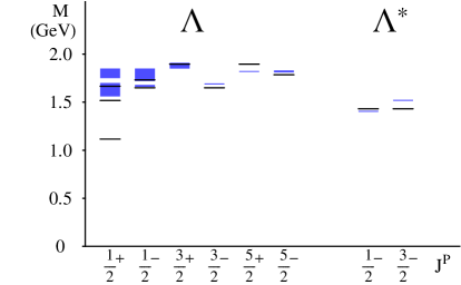
Figure 2: As Fig. 2, but for $\Lambda$ and $\Lambda^{*}$ resonances. Figure taken from Ref. qD2014b ; APS copyright.

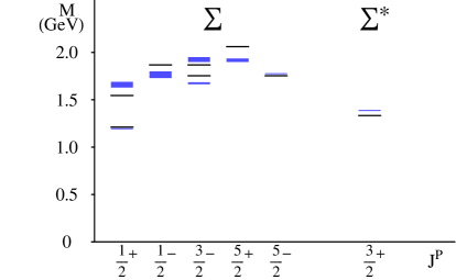
Figure 3: As Fig. 2, but for $\Sigma$ and $\Sigma^{*}$ resonances. Figure taken from Ref. qD2014b ; APS copyright.

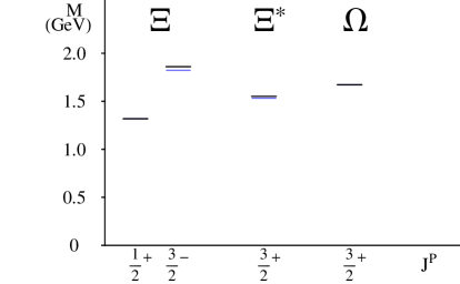
Figure 4: As Fig. 2, but for $\Xi$, $\Xi^{*}$ and $\Omega$ resonances. Figure taken from Ref. qD2014b ; APS copyright.

II.2 Nonstrange baryon spectrum with a spin-isospin transition interaction

In Ref. qD2014a , we improved the ”relativized” model of Ref. Ferretti:2011zz by introducing a spin-isospin transition interaction, which induces a mixing between scalar and axial-vector diquark states. We computed the nonstrange baryon spectrum within point form dynamics and used the resulting wave functions to calculate the magnetic moments of the proton and neutron (see Sec. III.1).

The spin-isospin transition interaction, $M_{\rm tr}(r)$, was chosen as

$$M_{\rm tr}(r)=V_{0}\mbox{ }e^{-\frac{1}{2}\nu^{2}r^{2}}(\vec{s}_{2}\cdot\vec{S})(\vec{t}_{2}\cdot\vec{T})\mbox{ },$$ (6)

where $V_{0}$ and $\nu$ are free parameters and the matrix elements of the spin transition operator, $\vec{S}$, are defined as

$$\left\langle\right.s_{1}^{\prime},m_{s_{1}}^{\prime}\left.\right|S_{\mu}^{[1]}\left|s_{1},m_{s_{1}}\right\rangle\neq 0\mbox{ for }s_{1}^{\prime}\neq s_{1}\mbox{ },$$ (7)

with $\left\langle 1\right\|S_{1}\left\|0\right\rangle=1$ and $\left\langle 0\right\|S_{1}\left\|1\right\rangle=-1$. The matrix elements of the isospin transition operator, $\vec{T}$, are defined analogously.

Figure 5: Comparison between the calculated masses (black lines) of the $3^{*}$ and $4^{*}$ nonstrange baryon resonances (up to 2 GeV) and the experimental masses from PDG Nakamura:2010zzi (boxes). Figure taken from Ref. qD2014a ; Società Italiana di Fisica/Springer-Verlag copyright.

The spin-isospin transition interaction of Eq. (6) mixes quark-scalar diquark and quark-axial-vector diquark states, i.e. states with $s_{1}=0$ ($t_{1}=0$) and $s_{1}=1$ ($t_{1}=1$), whose total spin (isospin) is $S=\frac{1}{2}$ ($T=\frac{1}{2}$). Thus, in this version of the model the nucleon state, as well as states such as the $D_{13}(1520)$, the $S_{11}(1535)$ and the $P_{11}(1440)$, contain both a $s_{1}=0$ and a $s_{1}=1$ component.

The introduction of the interaction of Eq. (6) determines an improvement in the overall quality of the reproduction of the experimental data (considering only $3^{*}$ and $4^{*}$ resonances) qD2014a , with respect to that obtained with the previous version of this model Ferretti:2011zz . In particular, the Roper resonance, $N(1440)$ $P_{11}$, is far better reproduced than before and the same holds for $N(1680)$ $F_{15}$. See Fig. 5.

III Baryon observables in the interacting quark-diquark model

Below, we discuss the formalism to calculate other baryon observables in the interacting quark-diquark model of Ref. qD2014a . We stress the importance of having a model in which $N^{*}$’s wave functions contain both a $q$–scalar diquark and a $q$–axial-vector diquark component, which play a role analogous to that of $\rho$- and $\lambda$-type components in the nucleon wave function. We think that the presence of both components is necessary to obtain a good reproduction of baryon observables in a quark-diquark model, including e.g. baryon magnetic moments and open-flavor strong decays.

III.1 Baryon magnetic moments

The electromagnetic response of the two-state diquark is in principle unknown.

As a starting point, for the magnetic dipole operator $\vec{\mu}$ we consider a non-relativistic expression qD2014a

$$\vec{\mu}=\frac{f}{m}\left(e_{1}\vec{s}_{1}+e_{2}\vec{s}_{2}\right)+\frac{f_{\rm q}}{m_{\rm q}}\mbox{ }e_{\rm q}\vec{s}_{\rm q}\mbox{ }.$$ (8)

In order to use the permutational symmetry of the quarks 1 and 2 of the diquark, we re-write Eq. (8) as qD2014a :

$$\vec{\mu}=\frac{f}{2m}\mbox{ }e_{\rm D}\vec{s}_{\rm D}+\frac{f}{2m}\mbox{ }\Delta e_{\rm D}\Delta\vec{s}_{\rm D}+\frac{f_{\rm q}}{m_{\rm q}}\mbox{ }e_{\rm q}\vec{s}_{\rm q}\mbox{ },$$ (9)

where $e_{\rm D}=e_{1}+e_{2}$ is the charge operator of the diquark in the isospin space, $\vec{s}_{\rm D}=\vec{s}_{1}+\vec{s}_{2}$ represents its spin, $\Delta e_{\rm D}=e_{1}-e_{2}$ is the difference between the charges of quarks 1 and 2 and $\Delta\vec{s}_{\rm D}=\vec{s}_{1}-\vec{s}_{2}$ is the difference between the spin operators of the two quarks. Eq. (9) can be re-written as qD2014a

$$\vec{\mu}=\frac{f_{\rm AV}}{m_{\rm AV}}\mbox{ }e_{\rm D}\vec{s}_{\rm D}+\frac{f_{\Delta}}{\left\langle m\right\rangle}\mbox{ }\Delta e_{\rm D}\Delta\vec{s}_{\rm D}+\frac{f_{\rm q}}{m_{\rm q}}\mbox{ }e_{\rm q}\vec{s}_{\rm q}\mbox{ },$$ (10)

representing the effective magnetic dipole operator of our model. Note that the second term gives the $S-AV$ transitions. The mean values of the effective dipole operator can be easily calculated, so that the numerical values of free parameters ($f_{\rm AV}$ and $f_{\Delta}$) can be fitted to reproduce the proton and neutron magnetic moments, that are $\mu_{\rm p}=2.793$ n.m.u. and $\mu_{\rm n}=-1.913$ n.m.u. Nakamura:2010zzi . Because the number of free parameters is larger than that of the experimental informations, we take $f_{\rm q}=1$; the resulting values for the other parameters are $f_{\rm AV}=0.0462$ and $f_{\Delta}=0.146$ qD2014a .

A more detailed study of the electromagnetic current will be carried out in a subsequent paper, with the aim of calculating the nucleon electromagnetic form factors and the helicity amplitudes of baryon resonances DeSanctis:TBP .

III.2 Open-flavor strong decays and missing resonances

As discussed in Refs. Santopinto:2004hw ; Ferretti:2011zz ; Galata:2012xt , the baryon spectra of quark-diquark and three quark models are quite distinct, the main differences being in the amount and energy of theoretically predicted states. When theoretical results and experimental observations are compared, it is clear that three quark models predict an eccessive number of states. This is the problem of missing resonances which can be, at least partially, solved in quark-diquark models in terms of a smaller number of effective degrees of freedom Santopinto:2004hw ; Ferretti:2011zz ; Galata:2012xt . Nevertheless, experimental informations on a hadron are not only limited to its mass, but also include (open- and hidden-flavor) strong decay widths, weak and e.m. radiative transitions, and so on. Thus, we think it is also worthwhile to compare three quark and quark-diquark model predictions for some of these observables.

Here, we discuss the formalism to compute the open-flavor strong decays of nonstrange baryons in the well-known ${}^{3}P_{0}$ pair-creation model Micu ; LeYaouanc ; Roberts:1992 . In the ${}^{3}P_{0}$ model, a hadron decay takes place in its rest frame and proceeds via the creation of an additional $q\bar{q}$ pair ($q_{1}$ and $q_{2}$) with vacuum quantum numbers, i.e. $J^{\rm PC}=0^{++}$. The decay amplitude $A(qD)\rightarrow B(Dq_{1})C(qq_{2})$ can be expressed as Micu ; LeYaouanc ; Roberts:1992

$$\Gamma_{A\rightarrow BC}=\Phi_{A\rightarrow BC}(q_{0})\sum_{\ell}\left|\left\langle BCq_{0}\,\ell J\right|T^{\dagger}\left|A\right\rangle\right|^{2}\mbox{ },$$ (11)

where $\mathcal{M}_{A\rightarrow BC}(q_{0})=\left\langle BCq_{0}\,\ell J\right|T^{\dagger}\left|A\right\rangle$ is the so-called ${}^{3}P_{0}$ amplitude, $\Phi_{A\rightarrow BC}(q_{0})$ the phase space factor for the decay, $q_{0}$ and $\ell$ the relative momentum and orbital angular momentum of the $BC$ pair. See Fig. 6. We write the phase space factor in the usual relativistic form, $\Phi_{A\rightarrow BC}(q_{0})=2\pi q_{0}\frac{E_{\rm b}(q_{0})E_{\rm c}(q_{0})}{M_{\rm a}}$, where $E_{\rm i}(q_{0})=\sqrt{q_{0}^{2}+M_{\rm i}^{2}}$ (i = $B,C$).

The transition operator of the ${}^{3}P_{0}$ model is given by Micu ; LeYaouanc ; Roberts:1992 :

$$\begin{array}[]{rcl}T^{\dagger}&=&-3\gamma_{0}\,\int d\vec{p}_{\rm q_{1}}\,d\vec{p}_{\rm q_{2}}\,\delta(\vec{p}_{\rm q_{1}}+\vec{p}_{\rm q_{2}})\,C_{12}\,F_{12}\,\Psi_{\rm d}(\vec{p}_{\rm q_{1}},\vec{p}_{\rm q_{2}})\left[\chi_{12}\,\times\,{\cal Y}_{1}(\vec{p}_{\rm q_{1}}-\vec{p}_{\rm q_{2}})\right]^{(0)}_{0}\\ &\times&b_{1}^{\dagger}(\vec{p}_{\rm q_{1}})\,d_{2}^{\dagger}(\vec{p}_{\rm q_{2}})\mbox{ }.\end{array}$$ (12)

Here, $\gamma_{0}$ is the pair-creation strength, $b_{1}^{\dagger}(\vec{p}_{\rm q_{1}})$ and $d_{2}^{\dagger}(\vec{p}_{\rm q_{2}})$ the creation operators for a quark and an antiquark with momenta $\vec{p}_{\rm q_{1}}$ and $\vec{p}_{\rm q_{2}}$, respectively, $\Psi_{\rm d}(\vec{p}_{\rm q_{1}},\vec{p}_{\rm q_{2}})$ the pair-creation vertex or quark form factor. The $q\bar{q}$ pair is characterized by a color singlet wave function $C_{12}$, a flavor singlet wave function $F_{12}$, a spin triplet wave function $\chi_{12}$ with spin $S=1$ and a solid spherical harmonic ${\cal Y}_{1}(\vec{p}_{\rm q_{1}}-\vec{p}_{\rm q_{2}})$, since the quark and antiquark are in a relative $P$ wave.

Figure 6: The ${}^{3}P_{0}$ pair-creation model of hadron vertices is here used within a quark-diquark picture for baryons. $D$ and $q$ are, respectively, the spectator diquark and quark; $q_{1}q_{2}$ is the created $q\bar{q}$ pair, with ${}^{3}P_{0}$ quantum numbers. Springer-Verlag Wien copyright.

III.3 Baryon spectrum with self-energy corrections in the quark-diquark model

The formalism described in the previous section can also be used to compute the baryon $\rightarrow$ baryon + meson vertices relevant to the calculation of baryon self-energies. For a calculation of octet and decuplet baryon self-energies within a three quark model, see Ref. baryon-SE .

We consider the Hamiltonian

$$H=H_{0}+V\mbox{ },$$ (13)

where $H_{0}$ is the ”unperturbed” part, describing the interaction between constituent (valence) quarks [see Eq. (1)], and $V$ the interaction which can couple a baryon state to the baryon-meson continuum. The physical mass of a baryon, $M_{\rm a}$, can be written as

$$M_{\rm a}=E_{\rm a}+\Sigma(E_{\rm a})\mbox{ },$$ (14)

where $E_{\rm a}$ is the bare mass, obtained by solving the eigenvalue problem of $H_{0}$, and

$$\Sigma(E_{\rm a})=\sum_{BC}\int_{0}^{\infty}q^{2}dq\mbox{ }\frac{\left|V_{\rm a,bc}(q)\right|^{2}}{E_{\rm a}-E_{\rm bc}}\mbox{ }$$ (15)

the self-energy correction. In Eq. (15), one has to sum over a complete set of baryon-meson intermediate states, $\left|BC\right\rangle$. These channels, with relative momentum $q$ between $B$ and $C$, have quantum numbers $J_{\rm bc}$ and $\ell$ coupled to the total angular momentum of the initial state $\left|A\right\rangle$. $V_{\rm a,bc}$ stands for the coupling between the intermediate state $\left|BC\right\rangle$ and the unperturbed wave function of the baryon $A$. Several choices for $V$ are possible, including the ${}^{3}P_{0}$ pair-creation model operator $T^{\dagger}$ of Eq. (12), which is ours.

In the following section, we provide an example of a ${}^{3}P_{0}$ model vertex calculation ($\Delta\rightarrow\Delta\pi$) in the quark-diquark model. This particular vertex provides the largest contribution to the $\Delta$ self-energy baryon-SE .

III.4 $\Delta\rightarrow\Delta\pi$ vertex

As an example, we briefly discuss the calculation of the $\Delta\rightarrow\Delta\pi$ vertex. The matrix elements can be calculated according to Refs. qD2014a ; Roberts:1992 ; Ferretti:2013faa ; Strong2015 , with a few differences. In the special case of $L_{\rm b}=L_{\rm c}=0$, the transition amplitude can be written as (Roberts:1992, , Sec. 6)

$$\begin{array}[]{rcl}\mathcal{M}_{A\rightarrow BC}&=&\frac{1}{3}(6\gamma_{0})\mbox{ }(-1)^{L_{\rm a}+S_{\rm a}+J_{\rm a}}\hat{S}_{\rm a}\hat{S}_{\rm b}\hat{S}_{\rm c}\hat{S}_{\rm bc}\hat{\ell}\left\{\begin{array}[]{ccc}S_{\rm D}&S_{\rm q_{1}}&S_{\rm b}\\ S_{\rm q}&S_{\rm q_{2}}&S_{\rm c}\\ S_{\rm a}&1&S_{\rm bc}\end{array}\right\}\left\{\begin{array}[]{ccc}S_{\rm a}&L_{\rm a}&J_{\rm a}\\ \ell&S_{\rm bc}&1\end{array}\right\}\\ &\times&\mathcal{F}_{A\rightarrow BC}\mbox{ }\epsilon_{A\rightarrow BC}(q_{0})\mbox{ },\end{array}$$ (16)

where $\mathcal{F}_{A\rightarrow BC}$ and $\epsilon_{A\rightarrow BC}(q_{0})$ are the flavor and spatial matrix elements, respectively, $\vec{S}_{\rm bc}=\vec{S}_{\rm b}+\vec{S}_{\rm c}$ the spin of the $BC$ pair, $S_{\rm D}$ and $S_{\rm q}$ the spin of the spectator diquark and quark, $S_{\rm q_{1}}$ and $S_{\rm q_{2}}$ the spins of the ${}^{3}P_{0}$ quark and antiquark. We also use the notation $\hat{\ell}=\sqrt{2\ell+1}$. In the $\Delta^{++}\rightarrow\Delta^{++}\pi^{0}$ case, Eq. (16) reduces to

$$\begin{array}[]{rcl}\mathcal{M}_{\Delta^{++}\rightarrow\Delta^{++}\pi^{0}}&=&-\frac{\gamma_{0}}{3\sqrt{5}}\mbox{ }\mathcal{F}_{\Delta^{++}\rightarrow\Delta^{++}\pi^{0}}\mbox{ }\epsilon_{\Delta^{++}\rightarrow\Delta^{++}\pi^{0}}(q_{0})\mbox{ },\end{array}$$ (17)

The flavor matrix element can be written as Ferretti:2013faa

$$\mathcal{F}_{A\rightarrow BC}=\left\langle BC|A\Phi_{0}\right\rangle\mbox{ },$$ (18)

where $\left|\Phi_{0}\right\rangle=\frac{1}{\sqrt{3}}\left(\left|u\bar{u}\right\rangle+\left|s\bar{s}\right\rangle+\left|s\bar{s}\right\rangle\right)$ is the SU(3) flavor singlet, $\left|A\right\rangle$, $\left|B\right\rangle$ and $\left|C\right\rangle$ the flavor wave functions of the corresponding hadrons Wilczek:2004im ; Jaffe:2004ph . In the $\Delta^{++}\rightarrow\Delta^{++}\pi^{0}$ case, Eq. (18) can be written as

$$\begin{array}[]{rcl}\mathcal{F}_{\Delta^{++}\rightarrow\Delta^{++}\pi^{0}}&=&\left\langle\Delta^{++}\pi^{0}|\Delta^{++}\Phi_{0}\right\rangle=\frac{1}{\sqrt{6}}\left[\left\langle\{u,u\}u\right|\otimes\left(\left\langle u\bar{u}\right|-\left\langle d\bar{d}\right|\right)\right]\\ &&\left[\left|\{u,u\}u\right\rangle\otimes\left(\left|u\bar{u}\right\rangle+\left|d\bar{d}\right\rangle+\left|s\bar{s}\right\rangle\right)\right]=\frac{1}{\sqrt{6}}\mbox{ },\end{array}$$ (19)

where $\left|\pi^{0}\right\rangle=\frac{1}{\sqrt{2}}$ $\left(\left|u\bar{u}\right\rangle-\left|d\bar{d}\right\rangle\right)$, $\left|\Delta^{++}\right\rangle=\left|\{u,u\}u\right\rangle$, and the notation $\{q,q\}$ stands for an axial-vector diquark Wilczek:2004im ; Jaffe:2004ph .

The spatial matrix element are the same as those for meson $\rightarrow$ meson + meson transitions Roberts:1992 ; Ferretti:2013faa . We use the coordinate system $\vec{q}_{\rm b}=\frac{1}{M_{\rm b}}\left(m_{\rm D}\vec{p}_{\rm q_{1}}-m_{\rm q_{1}}\vec{p}_{\rm D}\right)$, $\vec{q}_{\rm c}=\frac{1}{M_{\rm c}}\left(m_{\rm q_{2}}\vec{p}_{\rm q}-m_{\rm q}\vec{p}_{\rm q_{2}}\right)$, $\vec{P}_{\rm cm}=\vec{P}_{\rm b}+\vec{P}_{\rm c}$, $\vec{q}=\frac{M_{\rm c}}{M_{\rm bc}}\vec{P}_{\rm b}-\frac{M_{\rm b}}{M_{\rm bc}}\vec{P}_{\rm c}$, where $\vec{P}_{\rm b}=\vec{p}_{\rm D}+\vec{p}_{\rm q_{1}}$, $\vec{P}_{\rm c}=\vec{p}_{\rm q}+\vec{p}_{\rm q_{2}}$, $M_{\rm b}=m_{\rm D}+m_{\rm q_{1}}$, and $M_{\rm c}=m_{\rm q}+m_{\rm q_{2}}$. The spatial matrix elements can be written explicitly as

$$\begin{array}[]{rcl}\epsilon_{A\rightarrow BC}(\vec{p}_{\rm q},\vec{p}_{\rm D},\vec{p}_{\rm q_{1}},\vec{p}_{\rm q_{2}})&=&\int{\rm d}\vec{p}_{\rm q}{\rm d}\vec{p}_{\rm D}{\rm d}\vec{p}_{\rm q_{1}}{\rm d}\vec{p}_{\rm q_{2}}\mbox{ }\mathcal{Y}_{1}(\vec{p}_{\rm q_{1}}-\vec{p}_{\rm q_{2}})\delta(\vec{p}_{\rm q_{1}}+\vec{p}_{\rm q_{2}})\Psi_{\rm b}^{*}(\vec{p}_{\rm D},\vec{p}_{\rm q_{1}})\\ &\times&\Psi_{\rm c}^{*}(\vec{p}_{\rm q},\vec{p}_{\rm q_{2}})\Psi_{\rm d}(\vec{p}_{\rm q_{1}},\vec{p}_{\rm q_{2}})\Psi_{\rm a}(\vec{p}_{\rm q},\vec{p}_{\rm D})\mbox{ },\end{array}$$ (20)

where $\Psi_{\rm a}(\vec{p}_{\rm q},\vec{p}_{\rm D})=\Psi_{\rm a}^{\rm ho}\left(\frac{1}{M_{\rm a}}(m_{\rm D}\vec{p}_{\rm q}-m_{\rm q}\vec{p}_{\rm D})\right)\delta(\vec{P}_{\rm a}-\vec{p}_{\rm q}-\vec{p}_{\rm D})$, $\Psi_{\rm b}(\vec{p}_{\rm D},\vec{p}_{\rm q_{1}})=\Psi_{\rm b}^{\rm ho}\left(\vec{q}_{\rm b}\right)\delta(\vec{P}_{\rm b}-\vec{p}_{\rm D}-\vec{p}_{\rm q_{1}})$ and $\Psi_{\rm c}(\vec{p}_{\rm q},\vec{p}_{\rm q_{2}})=\Psi_{\rm c}^{\rm ho}\left(\vec{q}_{\rm c}\right)\delta(\vec{P}_{\rm c}-\vec{p}_{\rm q}-\vec{p}_{\rm q_{2}})$ are single harmonic oscillator (ho) wave functions with ho parameters $\alpha_{\rm a}=\alpha_{\rm b}=3.14$ GeV^-1 qD2014a and $\alpha_{\rm c}=2.00$ GeV^-1 Ackleh:1996yt ; $\Psi_{\rm d}(\vec{p}_{\rm q_{1}},\vec{p}_{\rm q_{2}})=\mbox{exp}\left[-\frac{\alpha_{\rm d}^{2}}{6}(\vec{p}_{\rm q_{1}}-\vec{p}_{\rm q_{2}})^{2}\right]$ is a Gaussian quark form factor, with $\alpha_{\rm d}=1.70$ GeV^-1 Ferretti:2013faa . In the case of ground-state hadrons, namely with no radial and orbital excitations, Eq. (20) reduces to

$$\begin{array}[]{rcl}\epsilon_{\Delta^{++}\rightarrow\Delta^{++}\pi^{0}}(q_{0})&=&-\mathcal{N}_{\rm a}\mathcal{N}_{\rm b}^{*}\mathcal{N}_{\rm c}^{*}\frac{x+1}{8G^{3}}q_{0}e^{-F^{2}q_{0}^{2}}\mbox{ },\end{array}$$ (21)

where

$$x=-\frac{\frac{m_{\rm D}}{M_{\rm b}}\alpha_{\rm b}^{2}+\frac{m_{\rm q}}{M_{\rm c}}\alpha_{\rm c}^{2}+\frac{4}{3}\alpha_{\rm d}^{2}}{\alpha_{\rm a}^{2}+\alpha_{\rm b}^{2}+\alpha_{\rm c}^{2}+\frac{4}{3}\alpha_{\rm d}^{2}}\mbox{ },$$ (22)

$$G^{2}=\frac{1}{2}\left(\alpha_{\rm a}^{2}+\alpha_{\rm b}^{2}+\alpha_{\rm c}^{2}+\frac{4}{3}\alpha_{\rm d}^{2}\right)\mbox{ },$$ (23)

$$F^{2}=\frac{1}{2}\left[\alpha_{\rm a}^{2}x^{2}+\alpha_{\rm b}^{2}\left(x+\frac{m_{\rm D}}{M_{\rm b}}\right)^{2}+\alpha_{\rm c}^{2}\left(x+\frac{m_{\rm q}}{M_{\rm c}}\right)^{2}+\frac{4}{3}\alpha_{\rm d}^{2}(x+1)^{2}\right]\mbox{ },$$ (24)

and $\mathcal{N}_{\rm i}=2\pi^{-1/4}\alpha_{\rm i}^{3/2}$ (i = a, b, c).

References

- (1) R. Jakob, P. J. Mulders and J. Rodrigues. Modelling quark distribution and fragmentation functions. Nucl. Phys. A 626: 937 (1997).
- (2) R. L. Jaffe and F. Wilczek. Diquarks and exotic spectroscopy. Phys. Rev. Lett. 91:232003 (2003).
- (3) F. Wilczek. Diquarks as inspiration and as objects. arXiv:hep-ph/0409168.
- (4) R. L. Jaffe. Exotica. Phys. Rept. 409:1 (2005).
- (5) E. Santopinto. An Interacting quark-diquark model of baryons. Phys. Rev. C 72:022201 (2005).
- (6) A. Selem and F. Wilczek. Hadron systematics and emergent diquarks. hep-ph/0602128.
- (7) J. Ferretti, A. Vassallo and E. Santopinto. Relativistic quark-diquark model of baryons. Phys. Rev. C 83:065204 (2011).
- (8) E. Santopinto and J. Ferretti, Strange and nonstrange baryon spectra in the relativistic interacting quark-diquark model with a Gürsey and Radicati-inspired exchange interaction. Phys. Rev. C 92:025202 (2015).
- (9) M. De Sanctis, J. Ferretti, E. Santopinto and A. Vassallo. Relativistic quark-diquark model of baryons with a spin-isospin transition interaction: Non-strange baryon spectrum and nucleon magnetic moments. Eur. Phys. J. A 52:121 (2016).
- (10) J. Ferretti, R. Magaña Vsevolodovna, E. Santopinto and P. Saracco. Charmed-baryon spectroscopy in the interacting quark-diquark model. Work in progress.
- (11) W. H. Klink. Relativistic simultaneously coupled multiparticle states. Phys. Rev. C 58:3617 (1998).
- (12) M. Gell-Mann. A Schematic Model of Baryons and Mesons. Phys. Lett. 8:214 (1964).
- (13) M. Ida and R. Kobayashi. Baryon resonances in a quark model. Prog. Theor. Phys. 36:846 (1966).
- (14) D. B. Lichtenberg and L. J. Tassie. Baryon Mass Splitting in a Boson-Fermion Model. Phys. Rev. 155:1601 (1967).
- (15) F. Gursey and L. A. Radicati. Spin and unitary spin independence of strong interactions. Phys. Rev. Lett. 13:173 (1964).
- (16) K. A. Olive et al. [Particle Data Group]. Review of Particle Physics. Chin. Phys. C 38:090001 (2014).
- (17) N. Isgur and G. Karl. P Wave Baryons in the Quark Model. Phys. Rev. D 18:4187 (1978); Positive Parity Excited Baryons in a Quark Model with Hyperfine Interactions. Phys. Rev. D 19:2653 (1979).
- (18) S. Capstick and N. Isgur. Baryons in a Relativized Quark Model with Chromodynamics. Phys. Rev. D 34:2809 (1986).
- (19) M. Ferraris et al.. A Three body force model for the baryon spectrum. Phys. Lett. B 364:231 (1995); M. Aiello et al.. A Three body force model for the electromagnetic excitation of the nucleon. Phys. Lett. B 387:215 (1996); M. M. Giannini and E. Santopinto. The hypercentral Constituent Quark Model and its application to baryon properties. Chin. J. Phys. 53:020301 (2015).
- (20) L. Y. Glozman and D. O. Riska. The Spectrum of the nucleons and the strange hyperons and chiral dynamics. Phys. Rep. 268:263 (1996).
- (21) U. Loring, B. C. Metsch and H. R. Petry. The Light baryon spectrum in a relativistic quark model with instanton induced quark forces: The Nonstrange baryon spectrum and ground states. Eur. Phys. J. A 10:395 (2001).
- (22) G. Galatà and E. Santopinto. Hybrid quark-diquark baryon model. Phys. Rev. C 86:045202 (2012).
- (23) C. Gutierrez and M. De Sanctis. A study of a relativistic quark-diquark model for the nucleon. Eur. Phys. J. A 50:169 (2014).
- (24) R. N. Faustov and V. O. Galkin. Strange baryon spectroscopy in the relativistic quark model. Phys. Rev. D 92:054005 (2015).
- (25) M. De Sanctis, J. Ferretti and E. Santopinto. Unpublished.
- (26) L. Micu. Decay rates of meson resonances in a quark model. Nucl. Phys. B 10:521 (1969).
- (27) A. Le Yaouanc, L. Oliver, O. Pene and J. -C. Raynal. Naive quark pair creation model of strong interaction vertices. Phys. Rev. D 8:2223 (1973); Naive quark pair creation model and baryon decays. Phys. Rev. D 9:1415 (1974).
- (28) W. Roberts and B. Silvestre-Brac. General method of calculation of any hadronic decay in the model. Few-Body Syst. 11:171 (1992).
- (29) H. García-Tecocoatzi, R. Bijker, J. Ferretti and E. Santopinto. arXiv:1603.07526.
- (30) J. Ferretti, G. Galatà and E. Santopinto. Interpretation of the as a charmonium state plus an extra component due to the coupling to the meson-meson continuum. Phys. Rev. C 88:015207 (2013).
- (31) R. Bijker, J. Ferretti, G. Galatà, H. García-Tecocoatzi and E. Santopinto. arXiv:1506.07469.
- (32) E. S. Ackleh, T. Barnes and E. S. Swanson. On the mechanism of open flavor strong decays. Phys. Rev. D 54:6811 (1996).