Double Higgcision:
125 GeV Higgs boson and a potential diphoton Resonance

Abstract

Searches for diphoton resonance have been shown to be very useful in discovering new heavy spin-0 or spin-2 particles. Supposing that a new heavy particle shows up in the diphoton channel and it points to a spin-0 boson, it can be allowed to have a small mixing with the observed 125 GeV Higgs-like boson. We borrow the example of the 750 GeV particles hinted with 3.2 fb^-1 data at the end of 2015 (though it did not appear in the 2016 data) to perform an analysis of “double Higgcision”. In this work, we perform a complete Higgs-signal strength analysis in the Higgs-portal type framework, using all the existing 125 GeV Higgs boson data as well as the diphoton signal strength of the 750 GeV scalar boson. The best fit prefers a very tiny mixing between two scalar bosons, which has to be accommodated in models for the 750 GeV scalar boson.

I Introduction

The first run at $\sqrt{s}=13$ TeV at the LHC has hinted a possibility of observing a new particle at around 750 GeV. Both ATLAS and CMS collaborations have reported a “bump” in the diphoton invariant mass distribution around 750 GeV, indicating a local significance of $3.9\sigma$ by ATLAS atlas and about $3\sigma$ by the CMS cms . Such an excitement has motivated a lot of speculations in many theories. Everyone has very high expectation for the new run coming up in May 2016 at the LHC.

Both ATLAS and CMS updated their findings in the early 2016 during the Moriond Conference. In particular, the CMS also included a set of data without the magnetic field into the analysis, and improved the significance to about $3.2\sigma$. The summary of the diphoton data of the 750 GeV resonance is given in Table 1. Although the hint is preliminary, it has stimulated a lot of phenomenological activities, bringing in a number of models for interpretation. If the particle decays directly into a pair of photons, it can have a spin-0 or spin-2, however, one has to entertain the possibility that the 750 GeV particle undergoes cascade decays into collimated photon objects (aka photon-jets) photon-jet .

During the ICHEP 2016 conference, both ATLAS and CMS reported their searches including the new 2016 data totaling about 12–13 fb^-1 ichep2016 . The ATLAS collaboration reanalyzed the 2015 data of 3.2 fb^-1 and they reported a little bit smaller excess of $3.4\sigma$ at 730 GeV, compared to the previous $3.9\sigma$ excess at 750 GeV. While, in the new 2016 data of 12.2 fb^-1, they have not observed any significant excess at all. In the combined data of 15.4 fb^-1, they observed $2.3\sigma$ excess at 710 GeV for the wide width case with $\Gamma_{X}/m_{X}$=10 %. In the narrow width case, the combined data show several $\sim 2\sigma$ excesses with the largest one at 1.6 TeV with a $2.4\sigma$ local significance. The CMS collaboration has observed no significant excess in proximity of 750 GeV in the new 2016 data of 12.9 fb^-1, either. But, interestingly, it reported the largest excess newly appeared at 620 GeV with $\sim 2.4-2.7\sigma$ local significance. And, like as in the ATLAS case, the combined $\sqrt{s}=13$ TeV data of 16.2/fb show several excesses at the level of $\sim 2\sigma$.

Both experiments did not further find evidence of the 750 GeV resonance. Nevertheless, we do not give up. Hints of new particles can easily show up in the near future data. For example, the CMS data in ICHEP 2016 showed a new $2\sigma$ effect at around 620–650 GeV. The ATLAS, on the other hand, did not see any new diphoton resonance in the new 13 TeV data but still there was $3.4\sigma$ effect around 730 GeV in the 2015 data. Under this situation, there are often possibilities that potentially heavy diphoton resonances can show up in the near future. We borrow the example of the 750 GeV particles hinted with 3.2 fb^-1 data at the end of 2015 (though it did not appear in the 2016 data) to perform an analysis of “double Higgcision” – the precision-coupling analysis involving both Higgs bosons.

In this work, we focus on the interpretation that this 750 GeV particle is a scalar boson that links the SM sector with the hidden sector through the Higgs-portal type interactions, in which an $SU(2)$ isospin-singlet scalar boson mixes with the SM Higgs boson through an angle $\alpha$ Chpoi:2013wga . We assume after mixing the lighter boson is the observed SM-like Higgs boson $H_{1}$ at 125 GeV while the heavier one $H_{2}$ is the one hinted at 750 GeV. Thus, the 750 GeV scalar boson $H_{2}$ opens the window to another hidden world containing perhaps dark matter and other exotic particles.

In our previous global fits to the Higgs-portal type models with all the Higgs boson data from Run I portal before the hint of the 750 GeV boson, we have constrained the parameter space of a few Higgs-portal singlet-scalar models. In those models without non-SM contributions to the $h\gamma\gamma$ and $hgg$ vertices, the mixing angle is constrained to $\cos\alpha>0.86$ at 95% CL. However, in those models with vector-like leptons (quarks) the mixing angle can be relaxed to $\cos\alpha>0.83\;(0.7)$ at 95% CL. The implication was that the 750 GeV scalar boson $H_{2}$ can be produced in $gg$ fusion as if it were a 750 GeV SM Higgs boson but with a suppression factor $\sin^{2}\alpha$ if there are no vector-like quarks running in the $H_{2}gg$ vertex. Additional contributions arise when there are vector-like quarks running in the loop. Similarly, the decays of the scalar boson $H_{2}$ can be enhanced substantially into a pair of photons and gluons in the presence of vector-like fermions.

In an earlier attempt when the 750 GeV particle was first hinted, we performed such an analysis in the Higgs-portal framework that the 750 GeV boson $H_{2}$ interacts with the SM particles via the mixing angle with the 125 GeV Higgs boson and also via vector-like fermions earlier . Because the vector-like quarks carry electric and color charges while the vector-like leptons carry electric charges, the 750 GeV boson can be produced via gluon fusion and can also decay into a pair of photons and gluons. In earlier we used all the 125 GeV Higgs boson signal strength data and also the diphoton cross section of the 750 GeV boson to constrain the couplings of the 125 GeV Higgs boson, the mixing angle, and also on the extra loop contributions to the 750 GeV boson due to the vector-like fermions.

In this work, we extend the earlier analysis into a full-swing analysis, taking into account various combinations of 125 GeV Higgs couplings, the 750 GeV boson couplings to vector-like fermions, and the mixing angle. Improvements are summarized as follows.

1. We include the effects of vector-like fermions in gluon fusion production and

2. We include the non-standard decay modes for the 750 GeV boson.

3. We separately consider the choices of narrow and wide width for the 750 GeV boson. While the ATLAS data prefers a wide width, the CMS data prefers the narrow width.

The organization is as follows. In the next section, we describe briefly the framework of Higgs-portal models with vector-like fermions, including the production and decays of the 125 GeV and 750 GeV bosons. In Sec. III, we describe the Higgs boson and 750 GeV boson data that we use in our analysis, and We present the fits for various combinations of couplings and the mixing angle in Sec. IV. In Sec. V, we discuss the decay rates for the 750 GeV boson into other diboson channels ($WW,ZZ$ and $Z\gamma$) when the vector-like quarks in the loop are weak doublets and/or weak singlets with arbitrary $U(1)_{Y}$ hypercharges. Then we conclude in Sec. VI.

Special note: After we posted this preprint to arXiv, both ATLAS and CMS announced that they did not find evidence of the 750 GeV resonance in the new 2016 data. We, nevertheless, think this double-Higgcision study would still be a good exercise whenever another diphoton resonance shows up in the future data. In the following, we shall borrow the data of the 750 GeV particles recorded with 3.2 fb^-1 luminosity at the end of 2015 to perform an analysis of “double Higgcision” – the precision-coupling analysis involving both Higgs bosons.

II Formalism

Interpreting the $750$ GeV diphoton resonance as a scalar resonance generically involves at least two interaction eigenstates of $h$ and $s$: $h$ denotes the remnant of the SM Higgs doublet $H$ and $s$ the singlet or the remnant of additional Higgs doublets, triplets, etc. Then the two states $h$ and $s$ mix and result in the two mass eigenstates $H_{1,2}$. In the singlet case, for example, the mixing is generated from renormalizable potential terms such as

$$V\supset\mu\,s\,H^{\dagger}H+\frac{\lambda}{2}s^{2}H^{\dagger}H\,.$$

In this work, for concreteness, we concentrate on the singlet case.

II.1 Mixing and couplings

The mass eigenstates are related to the states $h$ and $s$ through an $SO(2)$ rotation as follows:

$$H_{1}=h\,\cos\alpha-s\,\sin\alpha\,;\ \ \ \ H_{2}=h\,\sin\alpha+s\,\cos\alpha\,$$ (1)

with $\cos\alpha$ and $\sin\alpha$ describing the mixing between the interaction eigenstates $h$ and $s$. In the limit of $\sin\alpha\to 0$, $H_{1}\,(H_{2})$ becomes the pure doublet (singlet) state. In this work, we are taking $H_{1}$ for the 125 GeV boson discovered at the 8-TeV LHC run and $H_{2}$ for the 750 GeV state hinted at the early 13-TeV LHC run. We are taking $\cos\alpha>0$ without loss of generality. For the detailed description of this class of models and also Higgs-portal models, we refer to Refs. Chpoi:2013wga ; portal .

In this class of models, the singlet field $s$ does not directly couple to the SM particles, but only through the mixing with the SM Higgs field at renormalizable level. The Yukawa interactions of $h$ and $s$ are described by

$$-{\cal L}_{Y}=h\sum_{f=t,b,\tau}\frac{m_{f}}{v}\bar{f}{f}+s\sum_{F=Q,L}\,g^{S}_{s\bar{F}F}\bar{F}F\,,$$ (2)

with $f$ denoting the 3rd-generation SM fermions and $F$ the extra vector-like fermions (VLFs): vector-like quarks (VLQs) and vector-like leptons (VLLs). Thus, the couplings of the two mass eigenstates $H_{1,2}$ to the SM fermions and VLFs are given by

$$-{\cal L}_{Y} = H_{1}\,\left[\cos\alpha\,\sum_{f=t,b,\tau}\frac{m_{f}}{v}\bar{f}{f}-\sin\alpha\,\sum_{F=Q,L}\,g^{S}_{s\bar{F}F}\bar{F}F\right]$$ (3)

$$+ H_{2}\,\left[\sin\alpha\,\sum_{f=t,b,\tau}\frac{m_{f}}{v}\bar{f}{f}+\cos\alpha\,\sum_{F=Q,L}\,g^{S}_{s\bar{F}F}\bar{F}F\right]\,.$$

Incidentally, the couplings to massive vector bosons $V=W,Z$ are given by

$${\cal L}_{HVV}=gM_{W}\left(W_{\mu}^{+}W^{-\mu}+\frac{1}{2c_{W}^{2}}Z_{\mu}Z^{\mu}\right)\left(\cos\alpha\,H_{1}\ +\ \sin\alpha\,H_{2}\right)\,.$$ (4)

The couplings of $H_{1,2}$ to two gluons, following the conventions and normalizations of Ref. Lee:2003nta , are given by

$$S_{H_{1}}^{g} = \cos\alpha\,S^{g\,({\rm SM})}_{H_{1}}-\sin\alpha\,S^{g\,(Q)}_{H_{1}}$$

$$\equiv \cos\alpha\,\sum_{f=t,b}\,F_{sf}(\tau_{1f})-\sin\alpha\,\sum_{Q}\,g^{S}_{s\bar{Q}Q}\,\frac{v}{m_{Q}}\,F_{sf}(\tau_{1Q})\,,$$

$$S_{H_{2}}^{g} = \sin\alpha\,S^{g\,({\rm SM})}_{H_{2}}+\cos\alpha\,S^{g\,(Q)}_{H_{2}}$$ (5)

$$\equiv \sin\alpha\,\sum_{f=t,b}\,F_{sf}(\tau_{2f})+\cos\alpha\,\sum_{Q}\,g^{S}_{s\bar{Q}Q}\,\frac{v}{m_{Q}}\,F_{sf}(\tau_{2Q})\,,$$

where $\tau_{ix}=M_{H_{i}}^{2}/4m_{x}^{2}$. We note that $S^{g\,({\rm SM})}_{H_{1}}\simeq 0.651+0.050\,i$ for $M_{H_{1}}=125.5$ GeV and $S^{g\,({\rm SM})}_{H_{2}}\simeq 0.291+0.744\,i$ for $M_{H_{2}}=750$ GeV. In the limit $\tau\to 0$, $F_{sf}(0)=2/3$. The mass of extra fermion $F$ may be fixed by the relation $m_{F}=v_{s}\,g^{S}_{s\bar{F}F}+m^{0}_{F}$ where $v_{s}$ denotes the VEV of the singlet $s$ while $m^{0}_{F}$ is generated from a different origin other than $v_{s}$ as in $-{\cal L}_{\rm mass}\supset m^{0}_{F}\bar{F}F$. We note that when $m^{0}_{Q}=0$, each contribution from a VLQ is not suppressed by $1/m_{Q}$ but by the common factor $1/v_{s}$.

Similarly, the couplings of $H_{1,2}$ to two photons are given by

$$S_{H_{1}}^{\gamma} = \cos\alpha\,S^{\gamma\,({\rm SM})}_{H_{1}}-\sin\alpha\,S^{\gamma\,(F)}_{H_{1}}$$

$$\equiv \cos\alpha\left[2\sum_{f=t,b,\tau}\,N_{C}Q_{f}^{2}F_{sf}(\tau_{1f})-F_{1}(\tau_{1W})\right]-\sin\alpha\left[2\sum_{F}\,N_{C}Q_{F}^{2}g^{S}_{s\bar{F}F}\,\frac{v}{m_{F}}\,F_{sf}(\tau_{1F})\right]\,,$$

$$S_{H_{2}}^{\gamma} = \sin\alpha\,S^{\gamma\,({\rm SM})}_{H_{2}}+\cos\alpha\,S^{\gamma\,(F)}_{H_{2}}$$

$$\equiv \sin\alpha\left[2\sum_{f=t,b,\tau}\,N_{C}Q_{f}^{2}F_{sf}(\tau_{2f})-F_{1}(\tau_{2W})\right]+\cos\alpha\left[2\sum_{F}\,N_{C}Q_{F}^{2}g^{S}_{s\bar{F}F}\,\frac{v}{m_{F}}\,F_{sf}(\tau_{2F})\right]\,,$$

where $N_{C}=3$ and $1$ for quarks and leptons, respectively, and $Q_{f,F}$ denote the electric charges of fermions in the unit of $e$. In the limit $\tau\to 0$, $F_{1}(0)=7$. We note that $S^{\gamma\,({\rm SM})}_{H_{1}}\simeq-6.55+0.039\,i$ for $M_{H_{1}}=125.5$ GeV and $S^{\gamma\,({\rm SM})}_{H_{2}}\simeq-0.94-0.043\,i$ for $M_{H_{2}}=750$ GeV.

II.2 Production and Decay

The production cross section of $H_{1,2}$ via the gluon-fusion process is given by

$$\sigma(gg\to H_{1,2})=\frac{|S^{g}_{H_{1,2}}|^{2}}{|S^{g\,({\rm SM})}_{H_{1,2}}|^{2}}\,\sigma_{\rm SM}(gg\to H_{1,2})$$ (7)

with $\sigma_{\rm SM}(gg\to H_{1})$ and $\sigma_{\rm SM}(gg\to H_{2})$ denoting the corresponding SM cross sections for $M_{H_{1}}=125.5$ GeV and $M_{H_{2}}=750$ GeV, respectively. We note that $\sigma_{\rm SM}(gg\to H_{2})\approx 750$ fb at $\sqrt{s}=13$ TeV.

The total decay widths of $H_{1,2}$ can be cast into the form

$$\Gamma_{H_{1}} = \cos^{2}\alpha\Gamma^{\rm SM}_{H_{1}}+\Delta\Gamma_{\rm vis}^{H_{1}\to\gamma\gamma,gg,Z\gamma}+\Gamma^{\rm non-SM}_{H_{1}}\,;$$

$$\Gamma_{H_{2}} = \sin^{2}\alpha\Gamma^{\rm SM}_{H_{2}}+\Delta\Gamma_{\rm vis}^{H_{2}\to\gamma\gamma,gg,Z\gamma}+\Gamma^{\rm non-SM}_{H_{2}}\,,$$ (8)

with $\Gamma^{\rm SM}_{H_{1}}\simeq 4$ MeV and $\Gamma^{\rm SM}_{H_{2}}\simeq 250$ GeV for the SM-like $H_{2}$ with $M_{H_{2}}=750$ GeV . And $\Gamma^{\rm non-SM}_{H_{1,2}}$ denote additional partial decay widths of $H_{1,2}$ into non-SM particles which could be either visible or invisible. If the only non-SM particles into which $H_{1,2}$ can decay are invisible, one may have

$$\Gamma^{\rm non-SM}_{H_{1}}=\Delta\Gamma^{H_{1}}_{\rm inv}\,;\ \ \ \Gamma^{\rm non-SM}_{H_{2}}=\Gamma(H_{2}\to H_{1}H_{1})+\Delta\Gamma^{H_{2}}_{\rm inv}\,.$$ (9)

We note that $\Gamma^{\rm non-SM}_{H_{2}}$ includes the $H_{2}$ decay into $H_{1}H_{1}$ by definition. As we shall show that a sizeable $\Delta\Gamma^{H_{2}}_{\rm inv}$ into invisible particles such as dark matters is required to accommodate a large $\Gamma_{H_{2}}={\cal O}(10)$ GeV.

The quantities $\Delta\Gamma_{\rm vis}^{H_{1,2}\to\gamma\gamma\,,gg}$ are given by

$$\Delta\Gamma^{H_{1}\to\gamma\gamma}_{\rm vis} = \frac{M_{H_{1}}^{3}\alpha^{2}}{256\pi^{3}v^{2}}\left[\left|S_{H_{1}}^{\gamma}\right|^{2}-\cos^{2}\alpha\left|S_{H_{1}}^{\gamma\,({\rm SM})}\right|^{2}\right]\,,$$

$$\Delta\Gamma^{H_{1}\to gg}_{\rm vis} = \left[1+\frac{\alpha_{s}}{\pi}\left(\frac{95}{4}-7\right)\right]\,\frac{M_{H_{1}}^{3}\alpha_{s}^{2}}{32\pi^{3}v^{2}}\left[\left|S_{H_{1}}^{g}\right|^{2}-\cos^{2}\alpha\left|S_{H_{1}}^{g\,({\rm SM})}\right|^{2}\right]\,,$$

$$\Delta\Gamma^{H_{2}\to\gamma\gamma}_{\rm vis} = \frac{M_{H_{2}}^{3}\alpha^{2}}{256\pi^{3}v^{2}}\left[\left|S_{H_{2}}^{\gamma}\right|^{2}-\sin^{2}\alpha\left|S_{H_{2}}^{\gamma\,({\rm SM})}\right|^{2}\right]\,,$$

$$\Delta\Gamma^{H_{2}\to gg}_{\rm vis} = \left[1+\frac{\alpha_{s}}{\pi}\left(\frac{95}{4}-7\right)\right]\,\frac{M_{H_{2}}^{3}\alpha_{s}^{2}}{32\pi^{3}v^{2}}\left[\left|S_{H_{2}}^{g}\right|^{2}-\sin^{2}\alpha\left|S_{H_{2}}^{g\,({\rm SM})}\right|^{2}\right]\,,$$ (10)

with $\alpha_{s}=\alpha_{s}(M_{H_{1\,(2)}})$ for $\Delta\Gamma^{H_{1\,(2)}\to gg}$.

Before closing this section, we comment on the loop-induced decay widths $\Delta\Gamma^{H_{2}\to Z\gamma}_{\rm vis}$. The Higgs couplings are given by

$$S^{Z\gamma}_{H_{1}}=\cos\alpha S^{Z\gamma(\rm SM)}_{H_{1}}-\sin\alpha S^{Z\gamma(\rm F)}_{H_{1}}\,;\ \ \ S^{Z\gamma}_{H_{2}}=\sin\alpha S^{Z\gamma(\rm SM)}_{H_{2}}+\cos\alpha S^{Z\gamma(\rm F)}_{H_{2}}\,,$$ (11)

with $S^{Z\gamma(\rm SM)}_{H_{1}}\simeq-11.042+0.010i$ and $S^{Z\gamma(\rm SM)}_{H_{2}}\simeq-0.0771-1.805i$. The contributions from VLFs are

$$S^{Z\gamma(\rm F)}_{H_{1,2}}=2\sum_{F}N_{C}Q_{F}\frac{2g_{Z\bar{F}F}}{s_{W}c_{W}}\left(g^{S}_{s\bar{F}F}\frac{v}{m_{F}}\right)m^{2}_{F}F^{(0)}_{f}(M^{2}_{H_{1,2}},m^{2}_{F}),$$ (12)

where $Q_{F}$ and the couplings $g_{Z\bar{F}F}$ are defined in the interactions

$$-{\cal L}=Q_{F}\;e\bar{F}\gamma^{\mu}FA_{\mu}+\frac{e}{s_{W}c_{W}}g_{Z\bar{F}F}\bar{F}\gamma^{\mu}FZ_{\mu}\,,$$

and we note $2m^{2}_{F}F^{(0)}_{f}(M^{2}_{H_{1,2}},m^{2}_{F})=F_{sf}(0)=2/3$ in the heavy $m_{F}$ limit, $m_{F}\to\infty$. Finally, the decay widths are given by

$$\Delta\Gamma^{H_{1}\rightarrow Z\gamma}_{\rm vis} = \frac{M^{3}_{H_{1}}\alpha^{2}}{128\pi^{3}v^{2}}\left(1-\frac{M^{2}_{Z}}{M^{2}_{H_{1}}}\right)^{3}\left[|S^{Z\gamma}_{H_{1}}|^{2}-\cos^{2}\alpha|S^{Z\gamma({\rm{SM}})}_{H_{1}}|^{2}\right]\,,$$

$$\Delta\Gamma^{H_{2}\rightarrow Z\gamma}_{\rm vis} = \frac{M^{3}_{H_{2}}\alpha^{2}}{128\pi^{3}v^{2}}\left(1-\frac{M^{2}_{Z}}{M^{2}_{H_{2}}}\right)^{3}\left[|S^{Z\gamma}_{H_{2}}|^{2}-\sin^{2}\alpha|S^{Z\gamma({\rm{SM}})}_{H_{2}}|^{2}\right]\,.$$ (13)

With no available independent information on the $g_{Z\bar{F}F}$ couplings, we neglect $\Delta\Gamma^{H_{1,2}\rightarrow Z\gamma}_{\rm vis}$ by taking $g_{Z\bar{F}F}=0$ when we perform global fits .

III Higgs Data

III.1 $H_{1}$ Data

For $H_{1}$ with $M_{H_{1}}=125.5$ GeV, we use the signal strength data from Refs. Cheung:2013kla ; Cheung:2014noa . The theoretical signal strengths may be written as

$$\widehat{\mu}({\cal P},{\cal D})\simeq\widehat{\mu}({\cal P})\ \widehat{\mu}({\cal D})\;,$$ (14)

where ${\cal P}={\rm ggF},{\rm VBF},VH_{1},ttH$ denote the $H_{1}$ production mechanisms: gluon fusion (ggF), vector-boson fusion (VBF), and associated productions with a $V=W/Z$ boson ($VH_{1}$) and top quarks ($ttH_{1}$) and ${\cal D}=\gamma\gamma$, $ZZ,$ $WW,$ $b\bar{b},$ $\tau\bar{\tau}$ the decay channels. Explicitly, we are taking

$$\widehat{\mu}({\rm ggF}) = |S^{g}_{H_{1}}|^{2}/|S^{g({\rm SM})}_{H_{1}}|^{2}\,,$$

$$\widehat{\mu}({\rm VBF}) = \widehat{\mu}(VH_{1})=\widehat{\mu}(ttH_{1})=\cos^{2}\alpha$$ (15)

with $V=Z,W$. For the decay part,

$$\widehat{\mu}({\cal D})=\frac{B(H_{1}\to{\cal D})}{B(H_{\rm SM}\to{\cal D})}$$ (16)

with

$$B(H_{1}\to\gamma\gamma)=\frac{\Gamma(H_{1}\to\gamma\gamma)}{\Gamma_{H_{1}}}=\frac{|S^{\gamma}_{H_{1}}|^{2}/|S^{\gamma({\rm SM})}_{H_{1}}|^{2}\,\Gamma(H_{\rm SM}\to\gamma\gamma)}{\cos^{2}\alpha\Gamma^{\rm SM}_{H_{1}}+\Delta\Gamma_{\rm vis}^{H_{1}\to\gamma\gamma,gg,Z\gamma}+\Gamma^{\rm non-SM}_{H_{1}}}$$ (17)

and

$$B(H_{1}\to{\cal D})=\frac{\Gamma(H_{1}\to{\cal D})}{\Gamma_{H_{1}}}=\frac{\cos^{2}\alpha\Gamma(H_{\rm SM}\to{\cal D})}{\cos^{2}\alpha\Gamma^{\rm SM}_{H_{1}}+\Delta\Gamma_{\rm vis}^{H_{1}\to\gamma\gamma,gg,Z\gamma}+\Gamma^{\rm non-SM}_{H_{1}}}$$ (18)

for ${\cal D}=ZZ,WW,b\bar{b}$ and $\tau\bar{\tau}$. If there are no VLF contributions to the $H_{1}$ couplings to photons and gluons or $S_{H_{1}}^{g(Q)}=S_{H_{1}}^{\gamma(F)}=0$, the signal strengths are simply given by

$$\widehat{\mu}({\cal P},{\cal D})\simeq\frac{\cos^{4}\alpha}{\cos^{2}\alpha+\Gamma^{\rm non-SM}_{H_{1}}/\Gamma^{\rm SM}_{H_{1}}}\,.$$ (19)

For more details, we refer to Ref. Cheung:2013kla .

III.2 $H_{2}$ Data

For $H_{2}$ with $M_{H_{2}}=750$ GeV, we adopt the following cross sections for the diphoton process $pp\to H_{2}\to\gamma\gamma$ measured at $\sqrt{s}=13$ TeV atlas2 ; cms2 in 2015:

$$\sigma^{\rm ATLAS} \approx 9.7\pm 3.2\,{\rm fb}~{}({\rm for\,broad\,width})\,,$$

$$\sigma^{\rm ATLAS} \approx 6.3\pm 2.4\,{\rm fb}~{}({\rm for\,narrow\,width})\,,$$

$$\sigma^{\rm CMS} \approx 6.3^{+4.2}_{-3.1}\,{\rm fb}\,.$$

We also include the $8$-TeV CMS data which correspond to the following cross section at $\sqrt{s}=13$ TeV

$$\sigma^{\rm CMS} \approx 3.5^{+2.2}_{-1.8}\,{\rm fb}\,.$$

In this work, we neglect the $8$-TeV ATLAS data since they do not give positive-definite cross section at $1$-$\sigma$ level. We note that the ATLAS Collaboration gave the cross sections for the broad- and narrow-width cases separately. For definiteness we apply the broad-width value when $\Gamma_{H_{2}}\geq 40\,{\rm GeV}$ and the narrow-width value when $\Gamma_{H_{2}}\leq 10\,{\rm GeV}$. However, we take the averaged value

$$\sigma^{\rm ATLAS} \approx 8.0\pm 2.8\,{\rm fb}~{}$$

for intermediate $\Gamma_{H_{2}}$ with $10\,{\rm GeV}<\Gamma_{H_{2}}<40\,{\rm GeV}$. Strictly speaking, the CMS values are applicable only for the narrow-width case but, with no available data, we apply the same value for the intermediate- and broad-width cases too. Table 1 summarizes the experimental values of the cross sections $\sigma(pp\to H_{2}\to\gamma\gamma)$ at $\sqrt{s}=13$ GeV used in this work.

Table 1: The experimental values of the cross sections $\sigma(pp\to H_{2}\to\gamma\gamma)\approx\sigma(pp\to H_{2})\times B(H_{2}\to\gamma\gamma)$ at $\sqrt{s}=13$ GeV.

		13 TeV Data	8 TeV Data
	$6.3\pm 2.4$ fb	for $\Gamma_{H_{2}}\leq 10$ GeV
ATLAS	$8.0\pm 2.8$ fb	for $10$ GeV $<\Gamma_{H_{2}}<40$ GeV
	$9.7\pm 3.2$ fb	for $\Gamma_{H_{2}}\geq 40$ GeV
CMS	$6.3^{+4.2}_{-3.1}$ fb		$3.5^{+2.2}_{-1.8}$ fb

In this analysis, we further take into account the following experimental constraints on the $H_{2}$ production and its subsequent decays:

• Diboson: $\left.\sigma(pp\rightarrow H_{2})\right|_{\sqrt{s}=13\,{\rm TeV}}\times B(H_{2}\rightarrow VV)\lesssim$ 150 fb atlas3

• $t\bar{t}$: $\left.\sigma(pp\rightarrow H_{2})\right|_{\sqrt{s}=8\,{\rm TeV}}\times B(H_{2}\rightarrow t\bar{t})\lesssim$ 0.5 pb atlas5

• Dijet: $\left.\sigma(pp\rightarrow H_{2})\right|_{\sqrt{s}=8\,{\rm TeV}}\times B(H_{2}\rightarrow gg)\lesssim$ 1 pb atlas6 .

We would like to comment on the constraint on $\Gamma(H_{2}\to H_{1}H_{1})$ from the combined 95% upper limit on $\sigma(gg\to H_{2})\times B(H_{2}\to H_{1}H_{1})\raisebox{-3.69899pt}{~{}\shortstack{$<$ \\ [-0.07cm] $\sim$}}~{}45$ fb at $\sqrt{s}=8$ TeV Aad:2015xja :

$$\Gamma(H_{2}\to H_{1}H_{1})\raisebox{-3.69899pt}{~{}\shortstack{$<$ \\ [-0.07cm] $\sim$}}~{}15\,{\rm GeV}\,\left(\frac{150\,{\rm fb}}{\sigma(gg\to H_{2})}\right)\,\left(\frac{\Gamma_{H_{2}}}{50\,{\rm GeV}}\right)$$ (20)

where we normalize the cross section $\sigma(gg\to H_{2})$ using the corresponding SM Higgs production cross section for $M_{H_{2}}=750$ GeV at $\sqrt{s}=8$ TeV or $\left.\sigma_{\rm SM}(gg\to H_{2})\right|_{\sqrt{s}=8\,{\rm TeV}}\simeq 150$ fb which is smaller by a factor of $4.693$ compared to $\left.\sigma_{\rm SM}(gg\to H_{2})\right|_{\sqrt{s}=13\,{\rm TeV}}$. If we parameterize the $H_{2}$-$H_{1}$-$H_{1}$ coupling as follows

$${\cal L}_{3H}=g_{211}\,v\,H_{2}H_{1}H_{1}$$ (21)

the constraint on $\Gamma(H_{2}\to H_{1}H_{1})$ can be translated on the constraint on the coupling $g_{211}$:

$$\frac{g_{211}^{2}}{4\pi}\raisebox{-3.69899pt}{~{}\shortstack{$<$ \\ [-0.07cm] $\sim$}}~{}0.4\,\left(\frac{150\,{\rm fb}}{\sigma(gg\to H_{2})}\right)\,\left(\frac{\Gamma_{H_{2}}}{50\,{\rm GeV}}\right)$$ (22)

using

$$\Gamma(H_{2}\rightarrow H_{1}H_{1})=\,\frac{v^{2}\,g_{211}^{2}}{8\,\pi\,M_{H_{2}}}\,\Bigg{(}1-\frac{4\,M_{H_{1}}^{2}}{M_{H_{2}}^{2}}\Bigg{)}^{\frac{1}{2}}\,.$$

With a model-dependent coupling $g_{211}$, we do not impose any experimental constraint from $\sigma(gg\to H_{2})\times B(H_{2}\to H_{1}H_{1})$. Instead, as we shall see, we include $\Gamma(H_{2}\to H_{1}H_{1})$ as a part of the free parameter which parameterizes non-SM decays of $H_{2}$, as in $\Gamma_{H_{2}}^{\rm non-SM}=\Gamma(H_{2}\to H_{1}H_{1})+\Delta\Gamma^{H_{2}}_{\rm inv}$, where the second term denotes additional partial decay widths of $H_{1}$ into invisible particles.

Finally, the vector-boson fusion (VBF) contribution to $H_{2}$ production is given by

$$\sigma^{\rm VBF}(pp\rightarrow H_{2}jj)=\sin^{2}\alpha\,\sigma^{\rm VBF}_{\rm SM}(pp\rightarrow H_{2}jj),$$ (23)

with $\sigma^{\rm VBF}_{\rm SM}(pp\rightarrow H_{2}jj)\simeq$ 130 fb with SM-like $H_{2}$ with mass 750 GeV at $\sqrt{s}=$13 TeV handbook . While the gluon fusion process gives $\sigma(gg\to H_{2})\sim 1250\,\cos^{2}\alpha\,|S^{g(Q)}_{H_{2}}|^{2}$ fb at $\sqrt{s}=13$ TeV. With $\sin^{2}\alpha\raisebox{-3.69899pt}{~{}\shortstack{$<$ \\ [-0.07cm] $\sim$}}~{}0.2$, as will be seen, and a possibly large value of $|S^{g(Q)}_{H_{2}}|\sim{\cal O}(1)$, we can safely ignore the VBF production of $H_{2}$ in this work.

IV Fits

In our approach, without loss of generality, we have the following 7 model-independent parameters:

$$\sin\alpha\,;$$

$$S_{H_{2}}^{g(Q)}\,,\ \ \ S_{H_{2}}^{\gamma(F)}\,,\ \ \ \Gamma^{\rm non-SM}_{H_{2}}\,;$$

$$S_{H_{1}}^{g(Q)}\,,\ \ \ S_{H_{1}}^{\gamma(F)}\,,\ \ \ \Gamma^{\rm non-SM}_{H_{1}}\,.$$ (24)

In our numerical analysis, we shall restrict ourselves to the case $2m_{F}>M_{H_{2}}$ so that $H_{2}\to F\bar{F}$ decays are kinematically forbidden and $S^{g(Q),\gamma(F)}_{H_{1},H_{2}}$ are all real. Furthermore, we note that

$$S_{H_{1}}^{g(Q)} = \sum_{Q}g^{S}_{s\bar{Q}Q}\frac{v}{m_{Q}}F_{sf}(\tau_{1Q})\simeq\frac{2}{3}\sum_{Q}g^{S}_{s\bar{Q}Q}\frac{v}{m_{Q}}\,,$$

$$S_{H_{1}}^{\gamma(F)} = 2\sum_{F}N_{C}Q_{F}^{2}g^{S}_{s\bar{F}F}\frac{v}{m_{F}}F_{sf}(\tau_{1F})\simeq\frac{4}{3}\sum_{F}N_{C}Q_{F}^{2}g^{S}_{s\bar{F}F}\frac{v}{m_{F}}\,,$$ (25)

since $F_{sf}(\tau_{1F})\simeq F_{sf}(0)=2/3$. This may imply $S^{g(Q),\gamma(F)}_{H_{1}}$ are not completely independent of $S^{g(Q),\gamma(F)}_{H_{2}}$. In the heavy $m_{F}$ limit $m_{F}\to\infty$, for example, $F_{sf}(\tau_{1F})=F_{sf}(\tau_{2F})=F_{sf}(0)=2/3$ and we have

$$S_{H_{1}}^{g(Q)}=S_{H_{2}}^{g(Q)}\,,\ \ \ S_{H_{1}}^{\gamma(F)}=S_{H_{2}}^{\gamma(F)}\,.$$ (26)

On the other hand, if all the VLFs are degenerate around $m_{F}\sim M_{H_{2}}/2$ or $F_{sf}(\tau_{2F})\simeq F_{sf}(1)=1$ and we have

$$S_{H_{1}}^{g(Q)}=\frac{2}{3}S_{H_{2}}^{g(Q)}\,,\ \ \ S_{H_{1}}^{\gamma(F)}=\frac{2}{3}S_{H_{2}}^{\gamma(F)}\,.$$ (27)

For convenience we introduce the parameters $\eta^{g(Q)}$ and $\eta^{\gamma(F)}$ are defined as in

$$S_{H_{1}}^{g(Q)}\equiv\eta^{g(Q)}S_{H_{2}}^{g(Q)}\,,\ \ \ S_{H_{1}}^{\gamma(F)}\equiv\eta^{\gamma(F)}S_{H_{2}}^{\gamma(F)}\,.$$ (28)

We note that $|\eta^{g(Q)}|$ and $|\eta^{\gamma(F)}|$ take on values between $2/3$ and $1$ if all the couplings $g_{s\bar{F}F}$ are either positive or negative, but in general can take on any values.

IV.1 F4 fits

We first consider the minimal F4 fit varying the following $4$ parameters:

$$\sin\alpha\,;\ \ S_{H_{2}}^{g(Q)}\,,\ \ S_{H_{2}}^{\gamma(F)}\,,\ \ \Gamma^{\rm non-SM}_{H_{2}}\,.$$ (29)

For the remaining parameters, first of all, we are taking $\Gamma^{\rm non-SM}_{H_{1}}=0$. For the $\eta$ parameters, we consider the three extreme possibilities as follows:

• F4-1 with $\eta^{g(Q)}=\eta^{\gamma(F)}=0$ : The VLFs are assumed not to contribute to the $H_{1}$ couplings to photons and gluons. In this case, the $H_{1}$ sector communicates with the $H_{2}$ sector only through the mixing angle $\sin\alpha$ and, accordingly, the signal strengths become $\widehat{\mu}({\cal P},{\cal D})\simeq\cos^{2}\alpha$ independently of the production mechanism ${\cal P}$ and the decay mode ${\cal D}$

• F4-2 with $\eta^{g(Q)}=\eta^{\gamma(F)}=2/3$ : The VLFs are assumed to be almost degenerate with their masses around $M_{H_{2}}/2$.

• F4-3 $\eta^{g(Q)}=\eta^{\gamma(F)}=1$ : All the VLFs are much heavier than $H_{2}$.

And, the regions of the varying F4-fit parameters are taken as follows:

• $|\sin\alpha|\leq 0.5$: We consider the 95% confidence level (CL ) limit of $\cos\alpha\raisebox{-3.69899pt}{~{}\shortstack{$>$ \\ [-0.07cm] $\sim$}}~{}0.86$ obtained from the global fits to Higgs-portal models using the current LHC $H_{1}$ data portal . We shall show that $|\sin\alpha|$ would be more stringently constrained in the F4-2 and F4-3 fits with non-zero $\eta^{g(Q)}$ and $\eta^{\gamma(F)}$.

• $|S^{g(Q)}_{H_{2}}|\leq 10$: We assume that $|S^{g(Q)}_{H_{2}}|$ cannot be larger than $10$. In order to achieve the maximal value of $S^{g(Q)}_{H_{2}}\sim 10$, for example, there should be more than $20$ VLQs with $m_{Q}\sim 500$ GeV and $g_{s\bar{Q}Q}\sim 1$. As we shall show, the $H_{2}$ dijet constraint gives $|S^{g(Q)}_{H_{2}}|\leq 7$.

• $|S^{\gamma(F)}_{H_{2}}|\leq 100$: We consider a 10 times larger region for $S^{\gamma(F)}_{H_{2}}$ compared to $S^{g(Q)}_{H_{2}}$ because of the possible enhancement factor $2N_{C}Q_{F}^{2}$ and additional contributions from VLLs to the $H_{2}$ couplings to photons.

• $\Gamma_{H_{2}}^{\rm non-SM}\raisebox{-3.69899pt}{~{}\shortstack{$<$ \\ [-0.07cm] $\sim$}}~{}50$ GeV: We restrict to the case in which the total width of $H_{2}$ does not exceed $50$ GeV

Table 2: Best-fit values of F4-1 with $\eta^{\gamma(F)}=\eta^{g(Q)}=0$ and $\Gamma_{H_{1}}^{\rm non-SM}=0$, and varying: $\sin\alpha\subset[-0.5:0.5],\,S_{H_{2}}^{g(Q)}\subset[-10:10],\,S_{H_{2}}^{\gamma(F)}\subset[-100:100],\,\Gamma^{\rm non-SM}_{H_{2}}/{\rm GeV}\subset[0:50]$. The decay widths are in units of GeV and the cross sections in units of fb. Other than the model parameters, the quantities shown are: $\Gamma_{H_{2}}$ for the total decay width of $H_{2}$, $C_{H_{1}}^{g,\gamma}\equiv|S_{H_{1}}^{g,\gamma}|/|S_{H_{1}}^{g({\rm SM}),\gamma({\rm SM})}|$, $\sigma(H_{2})\equiv\sigma(gg\rightarrow H_{2})$ at $\sqrt{s}=13$ TeV, and $\sigma(XX)\equiv\sigma(gg\rightarrow H_{2}\to XX)=\sigma(gg\rightarrow H_{2})\times B(H_{2}\rightarrow XX)$ at the same value of $\sqrt{s}$. The first line shows the best-fit values for the global minimum over the full range of $\Gamma_{H_{2}}$, whereas the second line shows the results for the broad-width case under the assumption of $\Gamma_{H_{2}}\geq$ 40 GeV.

Fits	$\chi^{2}_{\rm tot}$	$\chi^{2}_{H_{1}}$	$\chi^{2}_{H_{2}}$	Best-fit values
				$\sin\alpha$	$S_{H_{2}}^{\gamma(F)}$	$S_{H_{2}}^{g(Q)}$	$\Gamma^{\rm non-SM}_{H_{1}}$	$\Gamma^{\rm non-SM}_{H_{2}}$	$\eta^{\gamma(F)}$	$\eta^{g(Q)}$
F4-1	$17.692$	$16.764$	$0.929$	$-4.6\times 10^{-4}$	$55.583$	$-0.299$	$0$	$3.012$	$0$	$0$
	$19.363$	$16.764$	$2.600$	$4.4\times 10^{-4}$	$-45.897$	$1.466$	$0$	$46.191$	$0$	$0$

Best-fit values
$\Gamma_{H_{2}}$	$C^{\gamma}_{H_{1}}$	$C^{g}_{H_{1}}$	$\sigma(H_{2})$	$\sigma(\gamma\gamma)$	$\sigma(WW)$	$\sigma(ZZ)$	$\sigma(t\bar{t})$	$\sigma(gg)$
$3.164$	$1.00$	$1.00$	$111.9$	$5.105$	$0.00$	$0.00$	$0.00$	$0.28$
$46.480$	$1.00$	$1.00$	$2693$	$5.696$	$0.00$	$0.00$	$0.00$	$11.05$

Table 3: The same as in TABLE 2 but with $\eta^{\gamma(F)}=\eta^{g(Q)}=2/3$.

Fits	$\chi^{2}_{\rm tot}$	$\chi^{2}_{H_{1}}$	$\chi^{2}_{H_{2}}$	Best-fit values
				$\sin\alpha$	$S_{H_{2}}^{\gamma(F)}$	$S_{H_{2}}^{g(Q)}$	$\Gamma^{\rm non-SM}_{H_{1}}$	$\Gamma^{\rm non-SM}_{H_{2}}$	$\eta^{\gamma(F)}$	$\eta^{g(Q)}$
F4-2	$16.736$	$15.807$	$0.929$	$3.570\times 10^{-2}$	$29.400$	$0.329$	$0$	$0.777$	$2/3$	$2/3$
	$18.412$	$15.812$	$2.600$	$1.447\times 10^{-2}$	$74.395$	$0.893$	$0$	$45.55$	$2/3$	$2/3$

Best-fit values
$\Gamma_{H_{2}}$	$C^{\gamma}_{H_{1}}$	$C^{g}_{H_{1}}$	$\sigma(H_{2})$	$\sigma(\gamma\gamma)$	$\sigma(WW)$	$\sigma(ZZ)$	$\sigma(t\bar{t})$	$\sigma(gg)$
$1.146$	$1.105$	$0.987$	$144.9$	$5.085$	$20.83$	$10.21$	$4.84$	$1.30$
$45.93$	$1.108$	$0.987$	$1009$	$5.673$	$0.59$	$0.29$	$0.14$	$1.57$

Table 4: The same as in TABLE 2 but with $\eta^{\gamma(F)}=\eta^{g(Q)}=1$.

Fits	$\chi^{2}_{\rm tot}$	$\chi^{2}_{H_{1}}$	$\chi^{2}_{H_{2}}$	Best-fit values
				$\sin\alpha$	$S_{H_{2}}^{\gamma(F)}$	$S_{H_{2}}^{g(Q)}$	$\Gamma^{\rm non-SM}_{H_{1}}$	$\Gamma^{\rm non-SM}_{H_{2}}$	$\eta^{\gamma(F)}$	$\eta^{g(Q)}$
F4-3	$16.740$	$15.810$	$0.929$	$-2.193\times 10^{-2}$	$-32.203$	$-0.396$	$0$	$1.753$	$1$	$1$
	$18.413$	$15.813$	$2.600$	$-0.933\times 10^{-2}$	$-75.915$	$-0.857$	$0$	$43.50$	$1$	$1$

Best-fit values
$\Gamma_{H_{2}}$	$C^{\gamma}_{H_{1}}$	$C^{g}_{H_{1}}$	$\sigma(H_{2})$	$\sigma(\gamma\gamma)$	$\sigma(WW)$	$\sigma(ZZ)$	$\sigma(t\bar{t})$	$\sigma(gg)$
$1.936$	$1.106$	$0.986$	$203.5$	$5.082$	$6.53$	$3.20$	$1.52$	$1.51$
$43.85$	$1.107$	$0.988$	$926.5$	$5.686$	$0.24$	$0.12$	$0.06$	$1.39$

In Tables 2, 3, and 4, we show the best-fit values for the model parameters and miscellaneous quantities for the F4-1, F4-2, and F4-3 fit, respectively. We first note that the global minima occur for the small value of $\Gamma_{H_{2}}=1$-$3$ GeV though the larger widths are less preferred only by a small $\Delta\chi^{2}<2$. The broad-width minima under the assumption of $\Gamma_{H_{2}}>40$ GeV give $\Gamma_{H_{2}}\sim 45$ GeV. The best-fit values of $\sin\alpha$ are either small or vanishingly small, independent of $\eta^{g(Q),\gamma(F)}$.

The best-fit values for the cross section $\sigma(gg\to H_{2}\to\gamma\gamma)$ are $5.1$ fb and $5.7$ fb, again independent of $\eta^{g(Q),\gamma(F)}$, for the global and broad-width minima, respectively. We find that

$$\sigma(gg\to H_{2}\to\gamma\gamma)\simeq 0.06\,\frac{\left(S^{g(Q)}_{H_{2}}S^{\gamma(F)}_{H_{2}}\right)^{2}}{\Gamma_{H_{2}}/{\rm GeV}}\,\ {\rm fb}\,.$$ (30)

Incidentally, we find

$$\sigma(gg\to H_{2})\simeq 1250\,\left(S^{g(Q)}_{H_{2}}\right)^{2}\,\ {\rm fb}\,,$$ (31)

and

$$\sigma(gg\to H_{2}\to gg)\simeq 110\,\frac{\left(S^{g(Q)}_{H_{2}}\right)^{4}}{\Gamma_{H_{2}}/{\rm GeV}}\,\ {\rm fb}\,.$$ (32)

For the F4-2 and F4-3 fits

$$\sigma(gg\to H_{2}\to WW)\simeq 16.5\times 10^{4}\,\frac{\left(S^{g(Q)}_{H_{2}}\right)^{2}\,\sin^{2}\alpha}{\Gamma_{H_{2}}/{\rm GeV}}\,\ {\rm fb}\,,$$ (33)

and $\sigma(gg\to H_{2}\to ZZ)\sim\sigma(gg\to H_{2}\to WW)/2$ and and $\sigma(gg\to H_{2}\to t\bar{t})\sim\sigma(gg\to H_{2}\to WW)/4$. Finally,

$$C_{H_{1}}^{\gamma} = \left|\frac{S_{H_{1}}^{\gamma}}{S_{H_{1}}^{\gamma({\rm SM})}}\right|\simeq\left|1+\sin\alpha\frac{\eta^{\gamma(F)}S^{\gamma(F)}_{H_{2}}}{6.55}\right|\,,$$

$$C_{H_{1}}^{g} = \left|\frac{S_{H_{1}}^{g}}{S_{H_{1}}^{g({\rm SM})}}\right|\simeq\left|1-\sin\alpha\frac{\eta^{g(Q)}S^{g(Q)}_{H_{2}}}{0.653}\right|\,.$$ (34)

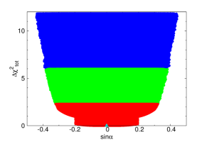
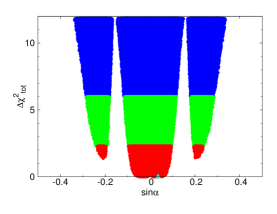
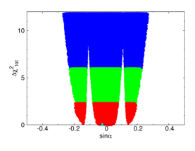
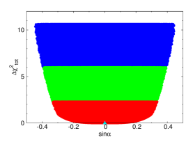
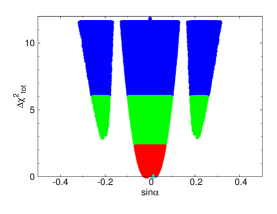
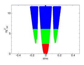
Figure 1: F4 fits: Plots of $\Delta\chi^{2}$ vs $\sin\alpha$ for the F4-1 (left), F4-2 (middle), and F4-3 (right) fits. In the upper row, we consider the full range of $\Gamma_{H_{2}}$ while, in the lower row, we consider the wide-width case requiring $\Gamma_{H_{2}}\geq$ 40 GeV. The regions shown are for $\Delta\chi^{2}=2.3$ (red), $5.99$ (green), and $11.83$ (blue) above the minimum. The triangles denote the corresponding minima.

Figure 1 shows $\Delta\chi^{2}$ vs $\sin\alpha$ for the F4-1 (left), F4-2 (middle), and F4-3 (right) fits. The upper frames show the results over the full range of $\Gamma_{H_{2}}$, while the lower frames show the results for the broad-width case under the assumption of $\Gamma_{H_{2}}\geq$ 40 GeV. The regions shown are for $\Delta\chi^{2}=2.3$ (red), $5.99$ (green), and $11.83$ (blue) above the minimum and the triangles denote the corresponding minima. First of all, we note that the minima occur at $\sin\alpha\sim 0$ in all the cases. Also, since $\Gamma_{H_{2}}\geq\sin^{2}\alpha\Gamma_{H_{2}}^{\rm SM}$, we observe

$$\sin^{2}\alpha\leq\frac{\Gamma_{H_{2}}}{\Gamma_{H_{2}}^{\rm SM}}$$ (35)

which implies, for example, $|\sin\alpha|\raisebox{-3.69899pt}{~{}\shortstack{$<$ \\ [-0.07cm] $\sim$}}~{}0.2\,(0.4)$ when $\Gamma_{H_{2}}\raisebox{-3.69899pt}{~{}\shortstack{$<$ \\ [-0.07cm] $\sim$}}~{}10\,(40)$ GeV and $|\sin\alpha|$ cannot exceed $\sim 0.45$ if $\Gamma_{H_{2}}\leq 50$ GeV. In the F4-1 fits, as shown in Table 2, the minimum for the full range of $\Gamma_{H_{2}}$ is deeper than that for the broad-width case. From the upper-left frame of Fig. 1, $|\sin\alpha|\raisebox{-3.69899pt}{~{}\shortstack{$<$ \\ [-0.07cm] $\sim$}}~{}0.2$ in the $\Delta\chi^{2}\raisebox{-3.69899pt}{~{}\shortstack{$<$ \\ [-0.07cm] $\sim$}}~{}1$ region and we find $\Gamma_{H_{2}}\raisebox{-3.69899pt}{~{}\shortstack{$<$ \\ [-0.07cm] $\sim$}}~{}10$ GeV there. In the F4-2 and F4-3 fits, in addition to the global minima at $\sin\alpha\sim 0$, two more local minima are developed at non-zero $\sin\alpha$. The local minima are developed at $|\sin\alpha|\simeq 0.20\,(0.13)$ for the F4-2 (F4-3) fits when $S_{H_{1}}^{\gamma}=-S^{\gamma\,({\rm SM})}_{H_{1}}$ and $|S^{\gamma\,(F)}_{H_{1}}|\simeq 100$, as we shall show soon.

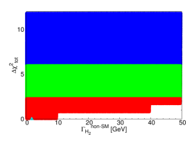
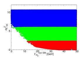
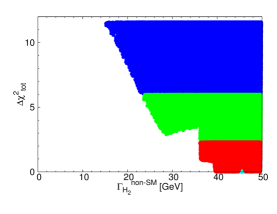
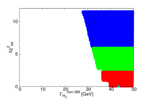
Figure 2: F4 fits: The same as in FIG. 1 but for $\Delta\chi^{2}$ vs $\Gamma_{H_{2}}^{\rm non-SM}$.

In Fig. 2 we show $\Delta\chi^{2}$ vs $\Gamma_{H_{2}}^{\rm non-SM}$ for the F4-1 (left), F4-2 (middle), and F4-3 (right) fits. Again, the upper frames are for the full range of $\Gamma_{H_{2}}$ while the lower ones for the broad-width case with $\Gamma_{H_{2}}\geq 40$ GeV. We do not see any dependence on $\eta^{g(Q)\,,\gamma(F)}$ in the upper frames since the $H_{2}$ width does not depend on them. The narrow width values are slightly preferred and $\Delta\chi^{2}=0$ is possible only when $\Gamma_{H_{2}}^{\rm non-SM}\raisebox{-3.69899pt}{~{}\shortstack{$<$ \\ [-0.07cm] $\sim$}}~{}10$ GeV. This is because the ATLAS data on $\sigma(pp\to H_{2}\to\gamma\gamma)$ are closer to the CMS data when $\Gamma_{H_{2}}\leq 10$ GeV, see Table 1. In the lower frames, we observe that, in the $\Delta\chi^{2}\leq 2.3$ region (red), $\Gamma_{H_{2}}^{\rm non-SM}\raisebox{-3.69899pt}{~{}\shortstack{$>$ \\ [-0.07cm] $\sim$}}~{}12$ GeV, $36$ GeV, and $36$ GeV to achieve $\Gamma_{H_{2}}\geq 40$ GeV for $\eta^{g(Q)\,,\gamma(F)}=0$ (F4-1, left), $\eta^{g(Q)\,,\gamma(F)}=2/3$ (F4-2, middle), and $\eta^{g(Q)\,,\gamma(F)}=1$ (F4-3, right), respectively.

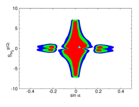
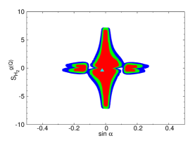
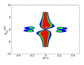
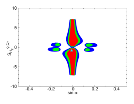
Figure 3: F4 fits: The CL regions for the F4-1 (left), F4-2 (middle), and F4-3 (right) fits in the $(\sin\alpha,S^{g(Q)}_{H_{2}})$ plane. In the upper row, we consider the full range of $\Gamma_{H_{2}}$ while, in the lower row, we consider the wide width case requiring $\Gamma_{H_{2}}\geq$ 40 GeV. In all the frames, we impose the diboson, $t\bar{t}$, and dijet constraints: $\sigma(pp\rightarrow H_{2})\times B(H_{2}\rightarrow VV)\lesssim$ 150 fb at 13 TeV, $\sigma(pp\rightarrow H_{2})\times B(H_{2}\rightarrow t\bar{t})\lesssim$ 0.5 pb at 8 TeV, and $\sigma(pp\rightarrow H_{2})\times B(H_{2}\rightarrow gg)\lesssim$ 1 pb at 8 TeV. The contour regions shown are for $\Delta\chi^{2}=2.3$ (red), $5.99$ (green), and $11.83$ (blue) above the minimum, which correspond to confidence levels of $68.3\%$, $95\%$, and $99.7\%$, respectively. The triangles in the upper row denote the minima over the full range of $\Gamma_{H_{2}}$, while those in the lower row the minima obtained under the assumption of $\Gamma_{H_{2}}\geq$ 40 GeV.

Figure 3 shows the CL regions in the $(\sin\alpha,S^{g(Q)}_{H_{2}})$ plane. When $\sin\alpha\sim 0$, $|S_{H_{2}}^{g(Q)}|$ is mostly constrained by $\left.\sigma(pp\to H_{2})\right|_{\sqrt{s}=8\,{\rm TeV}}\times B(H_{2}\to gg)\raisebox{-3.69899pt}{~{}\shortstack{$<$ \\ [-0.07cm] $\sim$}}~{}1$ pb. Using Eq. (32) and $\left.\sigma(gg\to H_{2})\right|_{\sqrt{s}=8\,{\rm TeV}}=\left.\sigma(gg\to H_{2})\right|_{\sqrt{s}=13\,{\rm TeV}}/4.7$, one may have $|S_{H_{2}}^{g(Q)}|\raisebox{-3.69899pt}{~{}\shortstack{$<$ \\ [-0.07cm] $\sim$}}~{}7\,(\Gamma_{H_{2}}/50\,{\rm GeV})^{1/4}$. As $\sin\alpha$ deviates from $0$, $|S_{H_{2}}^{g(Q)}|$ becomes constrained by $\left.\sigma(pp\to H_{2})\right|_{\sqrt{s}=13\,{\rm TeV}}\times B(H_{2}\to VV)\raisebox{-3.69899pt}{~{}\shortstack{$<$ \\ [-0.07cm] $\sim$}}~{}150$ fb. Using Eq. (33), one may have $|S_{H_{2}}^{g(Q)}\,\sin\alpha|\raisebox{-3.69899pt}{~{}\shortstack{$<$ \\ [-0.07cm] $\sim$}}~{}0.2\,(\Gamma_{H_{2}}/50\,{\rm GeV})^{1/2}$. These two observations mainly explain the shape of the CL regions in the left frames for F4-1 with $\eta^{g(Q)\,,\gamma(F)}=0$. For F4-2 and F4-3 with $\eta^{g(Q)\,,\gamma(F)}\neq 1$, the $H_{1}$ data provide additional constraints basically coming from $C_{H_{1}}^{g,\gamma}\sim 1$. Definitely, the CL regions populate along the $\sin\alpha=0$ line satisfying the $H_{1}$ constraints in the case $(S^{\gamma}_{H_{1}}\,,S^{g}_{H_{1}})\sim(+S^{\gamma({\rm SM})}_{H_{1}}\,,+S^{g({\rm SM})}_{H_{1}})$. On the other hand, the four islands around the points $\left(|\sin\alpha|=0.20\,,|S_{H_{2}}^{g(Q)}|=0.5\right)$ and $\left(|\sin\alpha|=0.13\,,|S_{H_{2}}^{g(Q)}|=0.5\right)$ for the F4-2 and F4-3 fits, respectively, satisfy the $H_{1}$ constraints in the case $(S^{\gamma}_{H_{1}}\,,S^{g}_{H_{1}})\sim(-S^{\gamma({\rm SM})}_{H_{1}}\,,+S^{g({\rm SM})}_{H_{1}})$. We find that the cases with $S^{g}_{H_{1}}\sim-S^{g({\rm SM})}_{H_{1}}$ cannot satisfy the $H_{1}$ constraints because it requires a too large value of $|S^{g(Q)}_{H_{2}}|\sim 10$  which is incompatible with the $H_{2}$ dijet constraint $|S^{g(Q)}_{H_{2}}|\raisebox{-3.69899pt}{~{}\shortstack{$<$ \\ [-0.07cm] $\sim$}}~{}7$ discussed before. Some numerical results on 68% CL regions are summarized in Table 5.

Table 5: The 68% CL regions of $\sigma(\gamma\gamma)=\sigma(gg\to H_{2})\times B(H_{2}\to\gamma\gamma)$, $\sin\alpha$, $\Gamma_{H_{2}}^{\rm non-SM}/{\rm GeV}$, $S^{g(Q)}_{H_{2}}$, and $S^{\gamma(F)}_{H_{2}}$ in the F4 fits.

Fits	$\eta^{g(Q),\gamma(F)}$	$\Gamma_{H_{2}}/$GeV	$\sigma(\gamma\gamma)/$fb	$|\sin\alpha|$	$\Gamma^{\rm non-SM}_{H_{2}}$	$|S^{g(Q)}_{H_{2}}|$	$|S^{\gamma(F)}_{H_{2}}|$
F4-1	0	0$\sim$50	2.9$\sim$7.4	0$\sim$0.33	0$\sim$50	0.05$\sim$7.0	2.2$\sim$100
	0	40$\sim$50	3.3$\sim$8.2	0$\sim$0.34	12$\sim$50	0.4$\sim$7.0	7.2$\sim$100
F4-2	2/3	0$\sim$50	2.9$\sim$7.4	0$\sim$0.095 or 0.20$\sim$0.24	0$\sim$50	0.05$\sim$6.6	2.4$\sim$100
	2/3	40$\sim$50	3.3$\sim$8.2	0$\sim$0.066	36$\sim$50	0.5$\sim$7.0	7.9$\sim$100
F4-3	1	0$\sim$50	2.9$\sim$7.4	0$\sim$0.077 or 0.13$\sim$0.20	0$\sim$50	0.05$\sim$6.6	2.4$\sim$100
	1	40$\sim$50	3.3$\sim$8.2	0$\sim$0.044	36$\sim$50	0.5$\sim$7.0	7.9$\sim$100

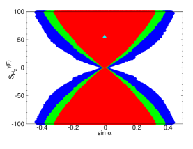
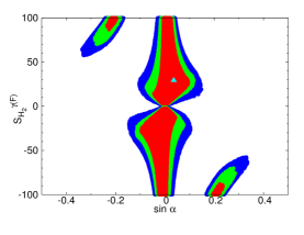
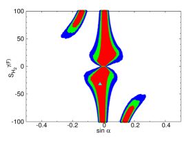
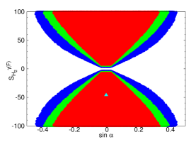
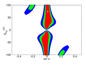
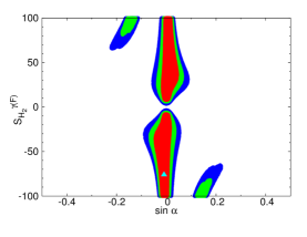
Figure 4: F4 fits: The same as in FIG. 3 but for the CL regions in the $(\sin\alpha,S^{\gamma(F)}_{H_{2}})$ plane.

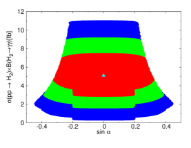
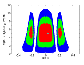
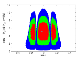
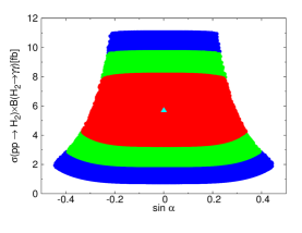
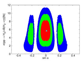
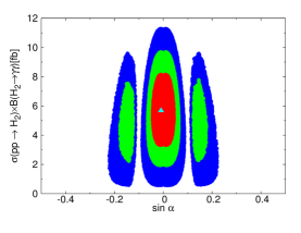
Figure 5: F4 fits: The same as in FIG. 3 but for the CL regions in the $(\sin\alpha,\sigma(gg\to H_{2})\times B(H_{2}\to\gamma\gamma)$ plane.

Figure 4 shows the CL regions in the $(\sin\alpha,S^{\gamma(F)}_{H_{2}})$ plane. For F4-1 with $\eta^{g(Q)\,,\gamma(F)}=0$, the parameter space is constrained basically by the lower limit on $\sigma(gg\to H_{2}\to\gamma\gamma)$. The lower limit $\sigma_{\rm min}\sim 3$ fb in at 68% CL, see Table 5. Then, using Eq. (30), we have $|S^{g(Q)}_{H_{2}}S^{\gamma(F)}_{H_{2}}|\raisebox{-3.69899pt}{~{}\shortstack{$>$ \\ [-0.07cm] $\sim$}}~{}50\,(\Gamma_{H_{2}}/50\,{\rm GeV})^{1/2}\,(\sigma_{\rm min}/3{\rm fb})^{1/2}$. Combining this with the the $H_{2}$ diboson constraint $|S_{H_{2}}^{g(Q)}\,\sin\alpha|\raisebox{-3.69899pt}{~{}\shortstack{$<$ \\ [-0.07cm] $\sim$}}~{}0.2\,(\Gamma_{H_{2}}/50\,{\rm GeV})^{1/2}$, we obtain $|S^{\gamma(F)}_{H_{2}}|\raisebox{-3.69899pt}{~{}\shortstack{$>$ \\ [-0.07cm] $\sim$}}~{}250\,|\sin\alpha|\,(\sigma_{\rm min}/3{\rm fb})^{1/2}$. This observation basically explains the shape of CL regions in the left frames together with the fact that the lower limit $\sigma_{\rm min}$ increases a little bit as $|\sin\alpha|$ deviates from $0$, see Fig. 5. For F4-2 and 4-3 with $\eta^{g(Q)\,,\gamma(F)}\neq 0$, on the other hand, the $H_{1}$ data gives further constraints like as in the $(\sin\alpha,S^{g(Q)}_{H_{2}})$ case. In the CL regions along the $\sin\alpha=0$ line, $(S^{\gamma}_{H_{1}}\,,S^{g}_{H_{1}})\sim(+S^{\gamma({\rm SM})}_{H_{1}}\,,+S^{g({\rm SM})}_{H_{1}})$. While, on the two islands at non-zero $\sin\alpha$ and for large values of $|S^{\gamma(F)}_{H_{2}}|$, $(S^{\gamma}_{H_{1}}\,,S^{g}_{H_{1}})\sim(-S^{\gamma({\rm SM})}_{H_{1}}\,,+S^{g({\rm SM})}_{H_{1}})$. When $S_{H_{1}}^{\gamma}=-S^{\gamma\,({\rm SM})}_{H_{1}}$, we have

$$\sin\alpha\,S^{\gamma\,(F)}_{H_{1}}=\sin\alpha\,\eta^{\gamma(F)}\,S^{\gamma\,(F)}_{H_{2}}=(1+\cos\alpha)S^{\gamma\,({\rm SM})}_{H_{1}}\simeq-13\,,$$ (36)

which implies that the local minima appear at $\sin\alpha\simeq-13/(\eta^{\gamma(F)}\,S^{\gamma\,(F)}_{H_{2}})$. When $S^{\gamma\,(F)}_{H_{2}}=\pm 100$, for example, the local minima may occur at $\sin\alpha\simeq\mp 0.20$ and $\mp 0.13$ for the F4-2 ($\eta^{\gamma(F)}=2/3$) and the F4-3 ($\eta^{\gamma(F)}=1$), respectively. This finally explains why the local minima are developed at $|\sin\alpha|\simeq 0.20\,(0.13)$ in the middle (right) frames of Fig. 1.

Figure 5 shows the CL regions in the $(\sin\alpha,\sigma(gg\to H_{2})\times B(H_{2}\to\gamma\gamma))$ plane. We observe the cross sections are centered around 5 fb.

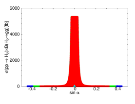
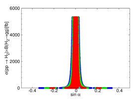
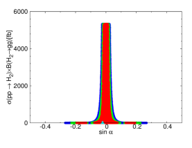
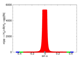
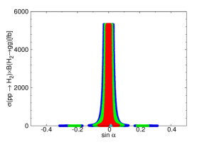
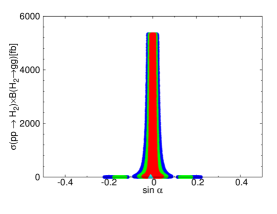
Figure 6: F4 fits: The same as in FIG. 3 but for the CL regions in the $(\sin\alpha,\sigma(gg\to H_{2})\times B(H_{2}\to gg)$ plane.

Figure 6 shows the CL regions in the $(\sin\alpha,\sigma(gg\to H_{2})\times B(H_{2}\to gg))$ plane. The cross section can be as large as up to $5$ pb around $\sin\alpha=0$, limited by the current $H_{2}$ dijet constraint.

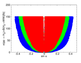
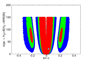
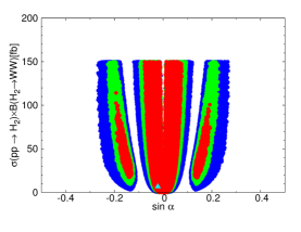
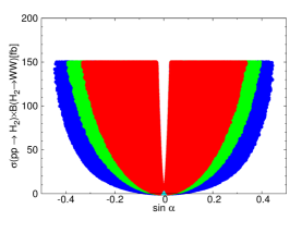
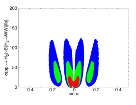
Figure 7: F4 fits: The same as in FIG. 3 but for the CL regions in the $(\sin\alpha,\sigma(gg\to H_{2})\times B(H_{2}\to WW)$ plane.

Figure 7 shows the CL regions in the $(\sin\alpha,\sigma(gg\to H_{2})\times B(H_{2}\to WW))$ plane. As $\sin\alpha$ deviates from $0$, the cross section can be as large as $150$ fb, limited by the current $H_{2}$ diboson constraint.

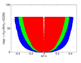
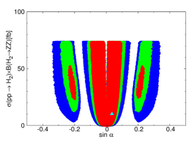
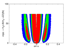
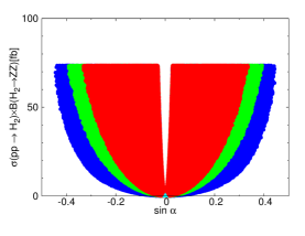
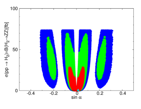
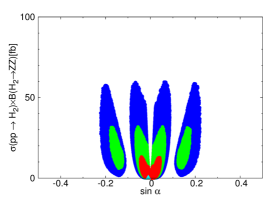
Figure 8: F4 fits: The same as in FIG. 3 but for the CL regions in the $(\sin\alpha,\sigma(gg\to H_{2})\times B(H_{2}\to ZZ)$ plane.

Compared to $\sigma(gg\to H_{2})\times B(H_{2}\to WW)$, the cross sections $\sigma(gg\to H_{2})\times B(H_{2}\to ZZ)$ and $\sigma(gg\to H_{2})\times B(H_{2}\to t\bar{t})$ can be as large as $70$ fb and $36$ fb, respectively, suppressed by the factors $B(H_{2}\to ZZ)/B(H_{2}\to WW)\sim 1/2$ and $B(H_{2}\to t\bar{t})/B(H_{2}\to WW)\sim 1/5$: see FIGs. 8 and  9. Otherwise, their patterns are similar.

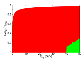
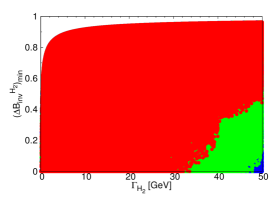
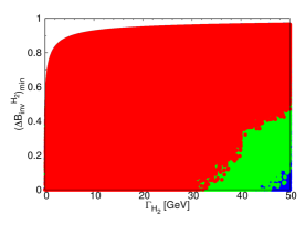
Figure 10: F4 fits: The CL regions for the F4-1 (left), F4-2 (middle), and F4-3 (right) fits in the $\left(\Gamma_{H_{2}},\left(\Delta B_{\rm inv}^{H_{2}}\right)_{\rm min}\right)$ plane. The colors are the same as in FIG. 3. See text for the definition of $\left(\Delta B_{\rm inv}^{H_{2}}\right)_{\rm min}$.

Finally, in FIG. 10, we show the CL regions in the $\left(\Gamma_{H_{2}},\left(\Delta B_{\rm inv}^{H_{2}}\right)_{\rm min}\right)$ plane where

$$\left(\Delta B^{H_{2}}_{\rm inv}\right)_{\rm min}\equiv\frac{\left(\Delta\Gamma^{H_{2}}_{\rm inv}\right)_{\rm min}}{\Gamma_{H_{2}}}$$

denoting the minimum value of the $H_{2}$ branching ratio into invisible particles. The minimum invisible decay width is obtained by requiring the decay width $\Gamma(H_{2}\to H_{1}H_{1})$ to saturate the current upper limit on $\sigma(gg\to H_{2})\times B(H_{2}\to H_{1}H_{2})$. More explicitly, we have

$$\left(\Delta\Gamma^{H_{2}}_{\rm inv}\right)_{\rm min}=\Gamma_{H_{2}}-\left[\sin^{2}\alpha\Gamma^{\rm SM}_{H_{2}}+\Delta\Gamma_{\rm vis}^{H_{2}\to\gamma\gamma}+\Delta\Gamma_{\rm vis}^{H_{2}\to gg}+\Gamma(H_{2}\to H_{1}H_{1})_{\rm max}\right]$$ (37)

with

$$\Gamma(H_{2}\to H_{1}H_{1})_{\rm max}=15\,{\rm GeV}\,\left(\frac{150\,{\rm fb}}{\left.\sigma(gg\to H_{2})\right|_{\sqrt{s}=8\,{\rm TeV}}}\right)\,\left(\frac{\Gamma_{H_{2}}}{50\,{\rm GeV}}\right)$$ (38)

where we again take $\left.\sigma(gg\to H_{2})\right|_{\sqrt{s}=8\,{\rm TeV}}=\left.\sigma(gg\to H_{2})\right|_{\sqrt{s}=13\,{\rm TeV}}/4.7$, see Eq. (20). We observe that, at 68% CL, $\left(\Delta B^{H_{2}}_{\rm inv}\right)_{\rm min}\sim 0$ can accommodate the situation with $\Gamma_{H_{2}}\raisebox{-3.69899pt}{~{}\shortstack{$<$ \\ [-0.07cm] $\sim$}}~{}40\,(32\,,32)$ GeV for F4-1 (F4-2, F4-3). But it should be larger than $\sim 0.2$ in order to accommodate the value $\Gamma_{H_{2}}\raisebox{-3.69899pt}{~{}\shortstack{$>$ \\ [-0.07cm] $\sim$}}~{}40$ GeV. Especially, when $\Gamma_{H_{2}}\sim 50$ GeV, the invisible branching ratio should be larger than $0.3$, $0.45$, and $0.45$ for F4-1, F4-2, and F4-3, respectively, at 68% CL.

V $H_{2}\to WW\,,ZZ\,,Z\gamma$

In this section, we consider the more general case in which there exist interactions between VLQs and $W/Z$ bosons. Then, even in the limit of $\sin\alpha=0$, $H_{2}$ can decay into $WW$ and $ZZ$ via VLQ loops and, more importantly, into $Z\gamma$.

Note that the couplings of VLQs to $W/Z$ bosons are highly model dependent on the weak isospin and the $U(1)_{Y}$ hypercharges. In order to be specific but without much loss of generality, we introduce $N_{d}$ copies of VLQ doublets $Q_{d}=(U,D)^{T}$ and $N_{s}$ copies of VLQ singlets $Q_{s}$ which couples to the SM gauge bosons as follows:

$$-{\cal L}_{\rm QCD} = g_{s}\left(\bar{U}\gamma^{\mu}T^{a}U+\bar{D}\gamma^{\mu}T^{a}D+\bar{Q}_{s}\gamma^{\mu}T^{a}Q_{s}\right)\,G^{a}_{\mu}\,,$$

$$-{\cal L}_{\rm EW} = \overline{Q_{d}}\gamma^{\mu}\left(g\frac{\tau^{a}}{2}W^{a}_{\mu}+g^{\prime}\frac{Y_{d}}{2}B_{\mu}\right)\,Q_{d}+\overline{Q_{s}}\gamma^{\mu}\left(g^{\prime}\frac{Y_{s}}{2}B_{\mu}\right)Q_{s}\,,$$ (39)

where $g_{s}$ denotes the $SU(3)$ gauge couping, $g=e/s_{W}$ and $g^{\prime}=e/c_{W}=gt_{W}$ with $s_{W}\equiv\sin\theta_{W}$, $c_{W}\equiv\cos\theta_{W}$, and $t_{W}=s_{W}/c_{W}$, and $T^{a}$ and $\tau^{a}/2$ are generators of $SU(3)$ and $SU(2)$ groups. And $Y_{d}$ and $Y_{s}$ denote the $U(1)_{Y}$ hypercharges of doublet $Q_{d}$ and singlet $Q_{s}$, respectively. They are related with the electric charges of VLQs by:

$$Q_{Q_{s}}=Y_{s}/2\,,\ \ \ Q_{U}=1/2+Y_{d}/2\,,\ \ \ Q_{D}=-1/2+Y_{d}/2\,.$$ (40)

Note that $Q_{U}-Q_{D}=1$ independently of $Y_{d}$. After rotating $(W_{\mu}^{3},B_{\mu})^{T}$ into $(Z_{\mu},A_{\mu})^{T}$ as usual or replacing $W_{\mu}^{3}$ and $B_{\mu}$ with $c_{W}Z_{\mu}+s_{W}A_{\mu}$ and $-s_{W}Z_{\mu}+c_{W}A_{\mu}$, respectively, one may have

$$-{\cal L}_{\rm EW} = e\left[Q_{U}\bar{U}\gamma^{\mu}U+Q_{D}\bar{D}\gamma^{\mu}D+Q_{Q_{s}}\bar{Q}_{s}\gamma^{\mu}Q_{s}\right]\,A_{\mu}$$ (41)

$$+ \frac{g}{c_{W}}\left[\bar{U}\gamma^{\mu}U\left(\frac{1}{2}-s_{W}^{2}Q_{U}\right)+\bar{D}\gamma^{\mu}D\left(-\frac{1}{2}-s_{W}^{2}Q_{D}\right)+\bar{Q}_{s}\gamma^{\mu}Q_{s}\left(-s_{W}^{2}Q_{Q_{s}}\right)\right]\,Z_{\mu}$$

$$+ \frac{g}{\sqrt{2}}(\bar{U}\gamma^{\mu}D\,W^{+}_{\mu}+\bar{D}\gamma^{\mu}U\,W^{-}_{\mu})\,.$$

We note the couplings to the $Z$ boson are purely vector-like and proportional to the factors $\pm 1/2-s_{W}^{2}Q_{U,D}$ which are different from the SM case where only the left-handed quarks are participating in the $SU(2)$ interaction. Further we note that the couplings to the $Z$ boson become the same as those to photons taking $(I_{3}^{F}-s_{W}^{2}Q_{F})/s_{W}c_{W}\,\to\,Q_{F}$ with $I_{3}^{U}=-I_{3}^{D}=1/2$ and $I_{3}^{Q_{s}}=0$. Incidentally, the Yukawa couplings of VLQs to the singlet $s$ are given by

$$-{\cal L}_{Y}=g^{S}_{s\bar{Q}_{d}Q_{d}}s\bar{Q}_{d}Q_{d}+g^{S}_{s\bar{Q}_{s}Q_{s}}s\bar{Q}_{s}Q_{s}\,.$$ (42)

With all these couplings given, one can calculate the VLQ-loop contributions to the $H_{2}$ couplings to $gg$, $\gamma\gamma$, $Z\gamma$, $ZZ$, and $WW$, which are proportional to $\cos\alpha$. For the $H_{2}$ couplings to two gluons and two photons, adopting the same notations as in Eqs. (II.1) and (II.1), we have

$$S^{g(Q)}_{H_{2}} = \sum_{Q_{d}}g^{S}_{s\bar{Q}_{d}Q_{d}}\left[\frac{v}{m_{U}}F_{sf}(\tau_{2U})+\frac{v}{m_{D}}F_{sf}(\tau_{2D})\right]+\sum_{Q_{s}}g^{S}_{s\bar{Q}_{s}Q_{s}}\frac{v}{m_{Q_{s}}}F_{sf}(\tau_{2Q_{s}})\;,$$ (43)

$$S^{\gamma(F)}_{H_{2}} = 2\sum_{Q_{d}}N_{C}g^{S}_{s\bar{Q}_{d}Q_{d}}\left[Q^{2}_{U}\frac{v}{m_{U}}F_{sf}(\tau_{2U})+Q^{2}_{D}\frac{v}{m_{D}}F_{sf}(\tau_{2D})\right]+2\sum_{Q_{s}}N_{C}g^{S}_{s\bar{Q}_{s}Q_{s}}Q^{2}_{Q_{s}}\frac{v}{m_{Q_{s}}}F_{sf}(\tau_{2Q_{s}})\;.$$

On the other hand, for the $H_{2}$ coupling to $Z$ and $\gamma$, following the convention of Eq. (11), we have

$$S^{Z\gamma(F)}_{H_{2}} = 2\sum_{Q_{d}}N_{C}g^{S}_{s\bar{Q}_{d}Q_{d}}\left\{Q_{U}\frac{(1/2-s^{2}_{W}Q_{U})}{s_{W}c_{W}}\frac{v}{m_{U}}\left[2m_{U}^{2}F^{(0)}_{f}(M_{H_{2}}^{2},m_{U}^{2})\right]\right.$$ (44)

$$\hskip 71.13188pt\left.+Q_{D}\frac{(-1/2-s^{2}_{W}Q_{D})}{s_{W}c_{W}}\frac{v}{m_{D}}\left[2m_{D}^{2}F^{(0)}_{f}(M_{H_{2}}^{2},m_{D}^{2})\right]\right\}$$

$$+ 2\sum_{Q_{s}}N_{C}g^{S}_{s\bar{Q}_{s}{Q_{s}}}\left\{Q_{Q_{s}}\frac{(-s^{2}_{W}Q_{Q_{s}})}{s_{W}c_{W}}\frac{v}{m_{Q_{s}}}\left[2m_{Q_{s}}^{2}F^{(0)}_{f}(M_{H_{2}}^{2},m_{Q_{s}}^{2})\right]\right\}\;.$$

Note that, in the limit of $M_{Z}=0$, we have $2m_{X}^{2}F^{(0)}_{f}(M_{H_{2}}^{2},m_{X}^{2})=F_{sf}(\tau_{2X})$ leading to $S^{Z\gamma(F)}_{H_{2}}=S^{\gamma(F)}_{H_{2}}$ after replacing $(I_{3}^{F}-s_{W}^{2}Q_{F})/s_{W}c_{W}$ with $Q_{F}$ as noted following Eq. (41).

For the decay processes $H_{2}\to VV$ with $V=W/Z$, the amplitude is given by

$${\cal M}_{VVH_{2}}=\sin\alpha{\cal M}_{VVH_{2}}^{(0)}+\cos\alpha{\cal M}_{VVH_{2}}^{(1)}$$ (45)

and, in the leading order neglecting the SM one-loop contributions to the $hWW$ vertex, the tree-level and one-loop amplitudes are

$${\cal M}^{(0)}_{WWH_{2}} = -gM_{W}\epsilon_{1}^{*}\cdot\epsilon_{2}^{*}\;,$$

$${\cal M}^{(0)}_{ZZH_{2}} = -\frac{gM_{W}}{c^{2}_{W}}\epsilon_{1}^{*}\cdot\epsilon_{2}^{*}\;,$$

$${\cal M}^{(1)}_{VVH_{2}} = -\frac{\alpha}{2\pi v}S^{VV(F)}_{H_{2}}\left[k_{1}\cdot k_{2}\,\epsilon_{1}^{*}\cdot\epsilon_{2}^{*}-k_{1}\cdot\epsilon_{2}^{*}\,k_{2}\cdot\epsilon_{1}^{*}\right]\;,$$ (46)

where $k_{1,2}$ are the momenta of the two massive vector bosons with $2k_{1}\cdot k_{2}=M_{H_{2}}^{2}-2M_{V}^{2}$ and $\epsilon_{1,2}$ are their polarization vectors. Note that there exists a tree-level contribution to the amplitude when $\sin\alpha\neq 0$ which has different vertex structure from the loop-induced one.

The form factor $S_{H_{2}}^{ZZ(F)}$ can be cast into the form

$$S^{ZZ(F)}_{H_{2}} = 2\sum_{Q_{d}}N_{C}g^{S}_{s\bar{Q}_{d}Q_{d}}\left\{\frac{(1/2-s_{W}^{2}Q_{U})^{2}}{s_{W}^{2}c_{W}^{2}}\frac{v}{m_{U}}\left[2m_{U}^{2}F_{f}^{(1)}(M_{H_{2}}^{2},m_{U}^{2})\right]\right.$$ (47)

$$\hskip 71.13188pt\left.+\frac{(-1/2-s_{W}^{2}Q_{D})^{2}}{s_{W}^{2}c_{W}^{2}}\frac{v}{m_{D}}\left[2m_{D}^{2}F_{f}^{(1)}(M_{H_{2}}^{2},m_{D}^{2})\right]\right\}$$

$$+ 2\sum_{Q_{s}}N_{C}g^{S}_{s\bar{Q}_{s}Q_{s}}\frac{(-s_{W}^{2}Q_{Q_{s}})^{2}}{s_{W}^{2}c_{W}^{2}}\frac{v}{m_{Q_{s}}}\left[2m_{Q_{s}}^{2}F_{f}^{(1)}(M_{H_{2}}^{2},m_{Q_{s}}^{2})\right]\,.$$

Note that, in the limit of $M_{Z}=0$, we have $2m_{X}^{2}F^{(1)}_{f}(M_{H_{2}}^{2},m_{X}^{2})=F_{sf}(\tau_{2X})$ leading to $S^{ZZ(F)}_{H_{2}}=S^{\gamma(F)}_{H_{2}}$ after replacing $(I_{3}^{F}-s_{W}^{2}Q_{F})/s_{W}c_{W}$ with $Q_{F}$, see Eq. (41).

Similarly, $S_{H_{2}}^{WW(F)}$ may take the form

$$S^{WW(F)}_{H_{2}} = 2\sum_{Q_{d}}N_{C}g^{S}_{s\bar{Q}_{d}Q_{d}}\frac{1}{2s^{2}_{W}}\frac{v}{m_{Q_{d}}}\left[2m^{2}_{Q_{d}}F^{(2)}_{f}(M_{H_{2}}^{2},m_{Q_{d}}^{2})\right]\;,$$ (48)

in the limit of $m_{U}=m_{D}=m_{Q_{d}}$. Also note that, in the limit of $M_{W}=0$, $2m_{Q_{d}}^{2}F^{(2)}_{f}(M_{H_{2}}^{2},m_{Q_{d}}^{2})=F_{sf}(\tau_{2{Q_{d}}})$ and $S^{WW(F)}_{H_{2}}$ becomes the same as the singlet contribution to $S^{\gamma(F)}_{H_{2}}$ after replacing $1/\sqrt{2}s_{W}$ with $Q_{Q_{s}}$ and, subsequently, $Q_{d}$ with $Q_{s}$.

In the previous section, we are taking $S_{H_{2}}^{\gamma(F)}$ and $S_{H_{2}}^{g(Q)}$ as our independent fitting parameters. In general, the form factors $S^{Z\gamma(F)}_{H_{2}}$, $S^{ZZ(F)}_{H_{2}}$, and $S^{WW(F)}_{H_{2}}$ are independent of $S_{H_{2}}^{\gamma(F)}$ and $S_{H_{2}}^{g(Q)}$ and they should be treated as independent parameters. But we find that they can be expressed in terms of $S_{H_{2}}^{\gamma(F)}$ and $S_{H_{2}}^{g(Q)}$ when

$$\frac{M_{Z,W}}{M_{H_{2}}}\rightarrow 0\,,\ \ \ g^{S}_{s\bar{Q}_{d}Q_{d}}=g^{S}_{s\bar{Q}_{s}Q_{s}}\,,\ \ \ m_{U}=m_{D}=m_{Q_{s}}\,.$$ (49)

In the above limit, we have

$$S^{Z\gamma(F)}_{H_{2}} = -t_{W}S^{\gamma(F)}_{H_{2}}+\left(\frac{N_{d}}{2N_{d}+N_{s}}\right)\frac{N_{C}}{s_{W}c_{W}}S^{g(Q)}_{H_{2}}\;,$$

$$S^{ZZ(F)}_{H_{2}} = t^{2}_{W}S^{\gamma(F)}_{H_{2}}+\left(\frac{N_{d}}{2N_{d}+N_{s}}\right)\frac{1-2s^{2}_{W}}{s^{2}_{W}c^{2}_{W}}N_{C}S^{g(Q)}_{H_{2}}\;,$$

$$S^{WW(F)}_{H_{2}} = \left(\frac{N_{d}}{2N_{d}+N_{s}}\right)\frac{N_{C}}{s^{2}_{W}}S^{g(Q)}_{H_{2}}\;,$$ (50)

where we use $Q_{U}-Q_{D}=1$. Note that the form factors $S^{Z\gamma(F)}_{H_{2}}$, $S^{ZZ(F)}_{H_{2}}$, and $S^{WW(F)}_{H_{2}}$ are all fixed once $S_{H_{2}}^{\gamma(F)}$, $S_{H_{2}}^{g(Q)}$, $N_{d}$, and $N_{s}$ are given and, accordingly, one can calculate the decay widths of $H_{2}$ into $Z\gamma$, $ZZ$, and $WW$, see Appendix A.

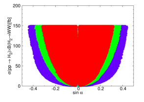
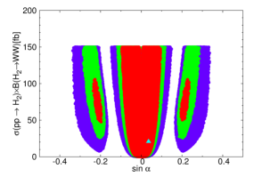
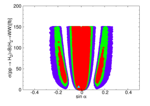
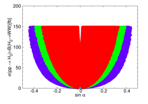
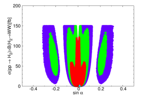
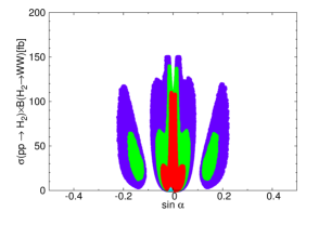
Figure 11: VLQ-W/Z: The same as in FIG. 7 but including the VLQ-loop induced contributions to $B(H_{2}\to WW)$ in the presence of interactions between VLQs and $W/Z$ bosons discussed in Section V. We are taking the limits in Eq. (49) and $N_{d}=N_{s}$.

In Fig. 11, we shows the CL regions in the $(\sin\alpha,\sigma(gg\to H_{2})\times B(H_{2}\to WW))$ plane including the VLQ-loop induced contributions to $B(H_{2}\to WW)$ in the presence of interactions between VLQs and $W/Z$ bosons. We are taking the limits suggested in Eq. (49) and $N_{d}=N_{s}$. Compared to Figure 7, we observe that there are non-vanishing VLF contributions to $\sigma(gg\to H_{2})\times B(H_{2}\to WW)$ when $\sin\alpha\to 0$ because:

$$\left.\Gamma(H_{2}\to WW)\right|_{\sin\alpha\to 0}\ \simeq\ \frac{M_{H_{2}}^{3}\alpha^{2}}{128\pi^{3}v^{2}}\left(S^{WW(F)}_{H_{2}}\right)^{2}\ =\ \frac{M_{H_{2}}^{3}\alpha^{2}}{128\pi^{3}v^{2}}\frac{\left(S^{g(Q)}_{H_{2}}\right)^{2}}{s_{W}^{4}}\,.$$ (51)

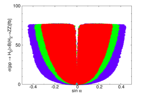
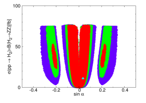
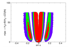
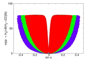
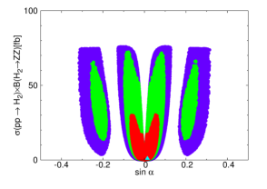
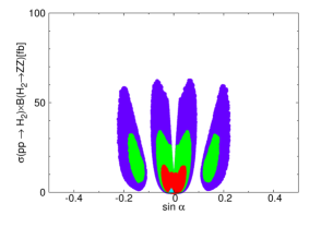
Figure 12: VLQ-W/Z: The same as in FIG. 8 but including the VLQ-loop induced contributions to $B(H_{2}\to ZZ)$ in the presence of interactions between VLQs and $W/Z$ bosons discussed in Section V. We are taking the limits in Eq. (49) and $N_{d}=N_{s}$.

Figure 12 shows the CL regions in the $(\sin\alpha,\sigma(gg\to H_{2})\times B(H_{2}\to ZZ))$ plane in the same context. Compared to Figure 8, we observe that there are also non-vanishing VLF contributions when $\sin\alpha\to 0$ because:

$$\left.\Gamma(H_{2}\to ZZ)\right|_{\sin\alpha\to 0}\ \simeq\ \frac{M_{H_{2}}^{3}\alpha^{2}}{256\pi^{3}v^{2}}\left(S^{ZZ(F)}_{H_{2}}\right)^{2}\ =\ \frac{M_{H_{2}}^{3}\alpha^{2}}{256\pi^{3}v^{2}}\left(t_{W}^{2}S^{\gamma(F)}_{H_{2}}+\frac{1-2s_{W}^{2}}{s_{W}^{2}c_{W}^{2}}S^{g(Q)}_{H_{2}}\right)^{2}\,.$$ (52)

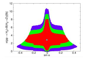
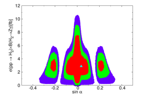
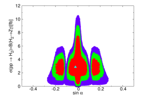
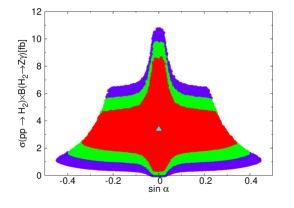
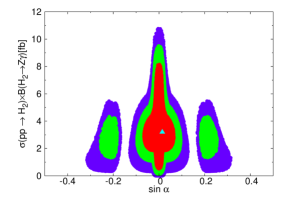
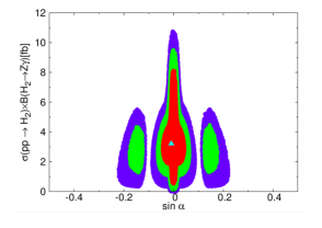
Figure 13: VLQ-W/Z: The same as in FIG. 3 but for the CL regions in the $(\sin\alpha,\sigma(gg\to H_{2})\times B(H_{2}\to Z\gamma))$ plane, including the VLQ-loop induced contributions in the presence of interactions between VLQs and $W/Z$ bosons discussed in Section V. We are taking the limits in Eq. (49) and $N_{d}=N_{s}$.

Figure 13 shows the CL regions in the $(\sin\alpha,\sigma(gg\to H_{2})\times B(H_{2}\to Z\gamma))$ plane. In the limits suggested in Eq. (49) with $N_{d}=N_{s}$, we have

$$\left.\Gamma(H_{2}\to Z\gamma)\right|_{\sin\alpha\to 0}\ \simeq\ \frac{M_{H_{2}}^{3}\alpha^{2}}{128\pi^{3}v^{2}}\left(S^{Z\gamma(F)}_{H_{2}}\right)^{2}\ =\ \frac{M_{H_{2}}^{3}\alpha^{2}}{128\pi^{3}v^{2}}\left(-t_{W}S^{\gamma(F)}_{H_{2}}+\frac{S^{g(Q)}_{H_{2}}}{s_{W}c_{W}}\right)^{2}\,.$$ (53)

We observe $\sigma(gg\to H_{2})\times B(H_{2}\to Z\gamma)$ can be as large as about $8$ fb around $\sin\alpha=0$ at 68 % CL.

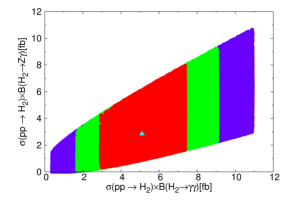
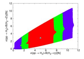
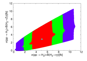
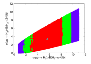
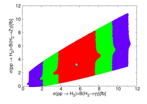
Figure 14: VLQ-W/Z: The CL regions for the correlations between $\sigma(gg\to H_{2})\times B(H_{2}\to\gamma\gamma)$ and $\sigma(gg\to H_{2})\times B(H_{2}\to Z\gamma)$ when $|\sin\alpha|<0.1$, including the VLQ-loop induced contributions in the presence of interactions between VLQs and $W/Z$ bosons discussed in Section V. We are taking the limits in Eq. (49) and $N_{d}=N_{s}$. The colors are the same as in FIG. 3.

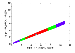
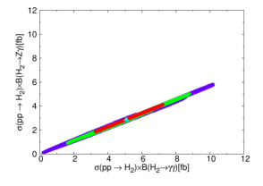
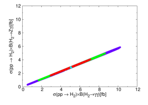
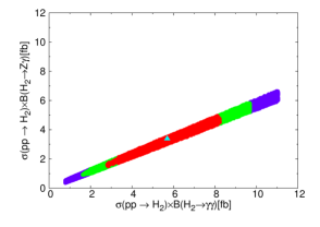
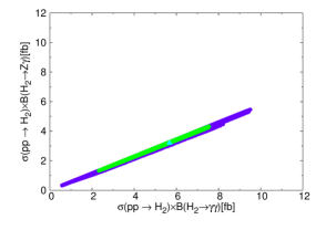
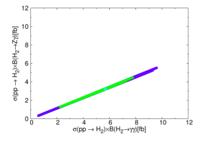
Figure 15: VLQ-W/Z: The same as in FIG. 14 but for $|\sin\alpha|\geq 0.1$.

In Figs. 14 and 15, we show the correlations between $\sigma(gg\to H_{2})\times B(H_{2}\to\gamma\gamma)$ and $\sigma(gg\to H_{2})\times B(H_{2}\to Z\gamma)$ taking $|\sin\alpha|<0.1$ and $|\sin\alpha|\geq 0.1$, respectively. In the limits suggested in Eq. (49) with $N_{d}=N_{s}$, we have

$$\left.\frac{\Gamma(H_{2}\to Z\gamma)}{\Gamma(H_{2}\to\gamma\gamma)}\right|_{\sin\alpha\to 0}\ \simeq\ 2\,\left(-t_{W}+\frac{1}{s_{W}c_{W}}\,\frac{S^{g(Q)}_{H_{2}}}{S^{\gamma(F)}_{H_{2}}}\right)^{2}\,.$$ (54)

When $|\sin\alpha|<0.1$, we observe

$$\frac{1}{5}\sigma(gg\to H_{2})\times B(H_{2}\to\gamma\gamma)\raisebox{-3.69899pt}{~{}\shortstack{$<$ \\ [-0.07cm] $\sim$}}~{}\sigma(gg\to H_{2})\times B(H_{2}\to Z\gamma)\raisebox{-3.69899pt}{~{}\shortstack{$<$ \\ [-0.07cm] $\sim$}}~{}\frac{4}{5}\,\sigma(gg\to H_{2})\times B(H_{2}\to\gamma\gamma)\ +\ 2\,{\rm fb}\,.$$ (55)

We find the correlation is strong when $|\sin\alpha|\geq 0.1$ and $|S^{g(Q)}_{H_{2}}/S^{\gamma(F)}_{H_{2}}|$ is small, see Figs. 3 and 4. In this case, we find

$$\frac{\sigma(gg\to H_{2})\times B(H_{2}\to Z\gamma)}{\sigma(gg\to H_{2})\times B(H_{2}\to\gamma\gamma)}\simeq 2t_{W}^{2}\simeq 2/3$$ (56)

as shown in Fig. 15 and indicated by Eq. (54).

VI Discussion

We have performed a “Double Higgcision” – Higgs precision study on both the 125 GeV Higgs boson and a potential diphoton resonance that may appear in the near future data. The recent 750 GeV diphoton resonance serves as a concrete example and we borrow the diphoton resonance data collected in 2015 in our analysis. We have used all the available Higgs boson data from 7 & 8 TeV runs as well as the diphoton cross sections of the 750 GeV boson from the 13 TeV run in 2015.

The important findings and a few comments are summarized as follows:

1. We have divided the analysis into two cases: (i) the width is varied freely and (ii) a broad-width defined by $\Gamma_{H_{2}}>40$ GeV is enforced. In the former case, a narrow width is always preferred and the width is of order $1-3$ GeV. On the other hand, in the broad-width case the width is around 45 GeV. Note that the minimal $\chi^{2}$ for these two cases only differ by a small amount, which is statistically not significant.

2. As we have shown that $S^{g(Q)}_{H_{1}}$ and $S^{g(Q)}_{H_{2}}$ and similarly $S^{\gamma(F)}_{H_{1}}$ and $S^{\gamma(F)}_{H_{2}}$ are independent parameters, but, however, they share the same form and with varying VLF mass their ratios $\eta^{g(Q)}$ and $\eta^{\gamma(F)}$ range between $2/3$ and $1$ for VLF mass from $m_{H_{2}}$ to infinity. We have shown the results of our analysis for these two representative values of $\eta$s in F4-2 and F4-3 fits, which have similar features.

3. We have also demonstrated the extreme case of $\eta$s equal to zero, i.e., the VLFs do not affect the gluon-fusion production of $H_{1}$ and the decays of $H_{1}$ into photons and gluons. In such a scenario, the effect of $H_{2}$ on $H_{1}$ Higgs boson data is only via the mixing angle $\cos\alpha$. Also, in the case the decays of $H_{2}$ into other modes such as $WW$, $ZZ$, and $t\bar{t}$ are only via the mixing with $H_{1}$. The best-fit shown allows a very tiny mixing angle $|\sin\alpha|\sim 10^{-4}$ such that the decays of $H_{2}\to WW,ZZ,t\bar{t}$ are negligible. If this is the case in the future data, there arises one immediate question why the mixing angle $\alpha$ is so tiny. This should be accommodated in any models for the 750 GeV diphoton excess.

4. In the fits of F4-2 and F4-3, the mixing angles are not too small and of order $10^{-2}$. The cross sections of $H_{2}$ into $WW,ZZ,t\bar{t}$ are not negligible and demonstrate the cross sections in the ratio of $4:2:1$, because of they are all proportional to the square of the SM couplings and $\sin\alpha$.

5. Both narrow and broad-width options in all three F4 fits, the $\Gamma^{\rm non-SM}_{H_{2}}$ dominates the total width $\Gamma_{H_{2}}$ of $H_{2}$, especially in the broad-width case the non-SM decay accounts for more than 99% branching ratio.

6. Should the $WW$, $ZZ$, $Z\gamma$ or $t\bar{t}$ modes of the $H_{2}$ be observed in near future, they would be extremely useful to tell the information on the VLFs.

7. If we assume that VLQs are weak isospin singlets and/or doublets, we can make more explicit and specific predictions on $H_{2}\rightarrow WW,ZZ,Z\gamma$, which are shown in Figs. 11-15. Discovery or upper bounds on the branching ratios of 750 GeV boson into these channels would shed more light on the nature of the VLQs in the loop. This could be complementary to the direct search for VLQs at the LHC through QCD interactions, keeping in mind that the decays of VLQs would be more model dependent.

8. Our procedure can be applied in the future discovery of a new resonance in the loop-induced diphoton and/or $Z\gamma$ channels, in particular, taking into account a possible mixing with the SM Higgs boson. Through this work, we demonstrate in detail how to carry out the relevant analysis in a proper way.

Appendix A Decay widths of $H_{2}$ into $Z\gamma$, $ZZ$, and $WW$

In this appendix, we present the explicit forms for the decay widths of $H_{2}$ into $Z\gamma$, $ZZ$, and $WW$ including the mixing between the SM Higgs boson and the singlet scalar.

The amplitude for the decay process $H_{2}\to Z(k_{1},\epsilon_{1})\ \gamma(k_{2},\epsilon_{2})$ can be written as

$${\cal M}_{Z\gamma H_{2}}=-\,\frac{\alpha}{2\pi v}\,S^{Z\gamma}_{H_{2}}\,\left[k_{1}\cdot k_{2}\,\epsilon_{1}^{*}\cdot\epsilon_{2}^{*}-k_{1}\cdot\epsilon_{2}^{*}\,k_{2}\cdot\epsilon_{1}^{*}\right]$$ (A.1)

where $k_{1,2}$ are the $4-$momenta of the $Z$ boson and the photon, respectively, and $\epsilon_{1,2}$ are their polarization vectors. We note that $2k_{1}\cdot k_{2}=M_{H_{2}}^{2}-M_{Z}^{2}$. The form factor $S^{Z\gamma}_{H_{2}}$ is given by the sum

$$S^{Z\gamma}_{H_{2}}=\sin{\alpha}S^{Z\gamma({\rm SM})}_{H_{2}}+\cos{\alpha}S^{Z\gamma(F)}_{H_{2}}$$

with $S^{Z\gamma({\rm SM})}_{H_{2}}\simeq-0.0771-1.805i$. The VLF contribution $S^{Z\gamma(F)}_{H_{2}}$ is model dependant and it is given by Eq. (44) in the context of $SU(2)_{L}$-doublet and singlet VLFs discussed in Section V. Then, the decay width of $H_{2}$ into $Z\gamma$ is given by

$$\Gamma(H_{2}\to Z\gamma)=\frac{M^{3}_{H_{2}}\alpha^{2}}{128\pi^{3}v^{2}}\left(1-\frac{M^{2}_{Z}}{M^{2}_{H_{2}}}\right)^{3}\left|S^{Z\gamma}_{H_{2}}\right|^{2}\;,$$ (A.2)

with

$$\left|S^{Z\gamma}_{H_{2}}\right|^{2}=\sin^{2}\alpha\,\left|S^{Z\gamma({\rm SM})}_{H_{2}}\right|^{2}+2\cos\alpha\sin\alpha\,S^{Z\gamma(F)}_{H_{2}}\,\Re{\rm e}\left({S^{Z\gamma({\rm SM})}_{H_{2}}}\right)+\cos^{2}\alpha\left(S^{Z\gamma(F)}_{H_{2}}\right)^{2}$$ (A.3)

assuming that the VLF mass satisfies $m_{F}>M_{H_{2}}/2$ so that $S^{Z\gamma(F)}_{H_{2}}$ becomes real.

The amplitude for the decay process $H_{2}\to V(k_{1},\epsilon_{1})\ V(k_{2},\epsilon_{2})$ can be written as

$${\cal M}_{VVH_{2}}=\sin\alpha{\cal M}_{VVH_{2}}^{(0)}+\cos\alpha{\cal M}_{VVH_{2}}^{(1)}\,.$$

In the leading order neglecting the SM one-loop contributions to the $hWW$ vertex, the tree-level and one-loop amplitudes are given by Eq. (V):

$${\cal M}^{(0)}_{WWH_{2}} = -gM_{W}\epsilon_{1}^{*}\cdot\epsilon_{2}^{*}\;,\ \ \ {\cal M}^{(0)}_{ZZH_{2}}=-\frac{gM_{W}}{c^{2}_{W}}\epsilon_{1}^{*}\cdot\epsilon_{2}^{*}\;;$$

$${\cal M}^{(1)}_{VVH_{2}} = -\frac{\alpha}{2\pi v}S^{VV(F)}_{H_{2}}\left[k_{1}\cdot k_{2}\,\epsilon_{1}^{*}\cdot\epsilon_{2}^{*}-k_{1}\cdot\epsilon_{2}^{*}\,k_{2}\cdot\epsilon_{1}^{*}\right]\;.$$

The VLF contributions $S^{ZZ(F)}_{H_{2}}$ and $S^{WW(F)}_{H_{2}}$ are model dependent and they are given by Eqs. (47) and (48), respectively, in the context discussed in Section V. Finally, the decay width of $H_{2}$ into $VV$ is given by

$$\Gamma(H_{2}\to VV)=\frac{\delta_{V}}{32\pi M_{H_{2}}}\sum|{\cal M}_{VVH_{2}}|^{2}\sqrt{1-\frac{4M^{2}_{V}}{M^{2}_{H_{2}}}}\;$$ (A.4)

with $\delta_{W}=2$ and $\delta_{Z}=1$. For the amplitude squared, explicitly, we obtain

$$\sum|{\cal M}_{WWH_{2}}|^{2} = \sin^{2}\alpha\,g^{2}M^{2}_{W}\left[3-\frac{M^{2}_{H_{2}}}{M^{2}_{W}}+\frac{M^{4}_{H_{2}}}{4M^{4}_{W}}\right]$$ (A.5)

$$+ \sin\alpha\,\cos\alpha\frac{gM_{W}\alpha}{\pi\,v}\left[-3M^{2}_{W}+\frac{3M^{2}_{H_{2}}}{2}\right]S^{WW(F)}_{H_{2}}$$

$$+ \cos^{2}\alpha\frac{\alpha^{2}}{4\pi^{2}\,v^{2}}\left[3M^{4}_{W}-2M^{2}_{W}M^{2}_{H_{2}}+\frac{M^{4}_{H_{2}}}{2}\right]\left(S^{WW(F)}_{H_{2}}\right)^{2}\;;$$

$$\sum|{\cal M}_{ZZH_{2}}|^{2} = \sin^{2}\alpha\,\frac{g^{2}M^{2}_{W}}{c^{4}_{W}}\left[3-\frac{M^{2}_{H_{2}}}{M^{2}_{Z}}+\frac{M^{4}_{H_{2}}}{4M^{4}_{Z}}\right]$$ (A.6)

$$+ \sin\alpha\,\cos\alpha\frac{gM_{W}\alpha}{c^{2}_{W}\pi\,v}\left[-3M^{2}_{Z}+\frac{3M^{2}_{H_{2}}}{2}\right]S^{ZZ(F)}_{H_{2}}$$

$$+ \cos^{2}\alpha\frac{\alpha^{2}}{4\pi^{2}\,v^{2}}\left[3M^{4}_{Z}-2M^{2}_{Z}M^{2}_{H_{2}}+\frac{M^{4}_{H_{2}}}{2}\right]\left(S^{ZZ(F)}_{H_{2}}\right)^{2}\;.$$

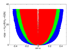
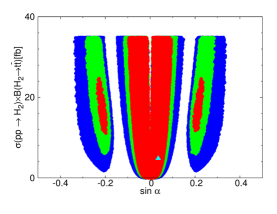
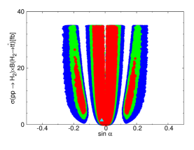
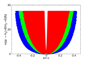
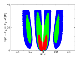
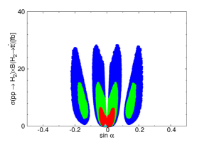
Figure 9: F4 fits: The same as in FIG. 3 but for the CL regions in the $(\sin\alpha,\sigma(gg\to H_{2})\times B(H_{2}\to t\bar{t})$ plane.

References

- (1) G. Aad et al. [ATLAS Collaboration], “Observation of a new particle in the search for the Standard Model Higgs boson with the ATLAS detector at the LHC,” Phys. Lett. B 716, 1 (2012) [arXiv:1207.7214 [hep-ex]].
- (2) S. Chatrchyan et al. [CMS Collaboration], “Observation of a new boson at a mass of 125 GeV with the CMS experiment at the LHC,” Phys. Lett. B 716, 30 (2012) [arXiv:1207.7235 [hep-ex]].
- (3) J. Chang, K. Cheung and C. T. Lu, Phys. Rev. D 93, no. 7, 075013 (2016) doi:10.1103/PhysRevD.93.075013 [arXiv:1512.06671 [hep-ph]].
- (4) B. Lenzi (ATLAS collabration), “Search for a high mass diphoton resonance using the ATLAS detector,” a talk at the 38th International Conference on High Energy Physics (ICHPE2016); C. Rovelli (CMS collaboration), “Search for BSM physics in di-photon final states at CMS,” a talk at the 38th International Conference on High Energy Physics (ICHPE2016).
- (5) S. Choi, S. Jung and P. Ko, “Implications of LHC data on 125 GeV Higgs-like boson for the Standard Model and its various extensions,” JHEP 1310 (2013) 225 [arXiv:1307.3948].
- (6) K. Cheung, P. Ko, J. S. Lee and P. Y. Tseng, JHEP 1510, 057 (2015) doi:10.1007/JHEP10(2015)057 [arXiv:1507.06158 [hep-ph]].
- (7) K. Cheung, P. Ko, J. S. Lee, J. Park and P. Y. Tseng, arXiv:1512.07853 [hep-ph].
- (8) J. S. Lee, A. Pilaftsis, M. S. Carena, S. Y. Choi, M. Drees, J. R. Ellis and C. E. M. Wagner, “CPsuperH: A Computational tool for Higgs phenomenology in the minimal supersymmetric standard model with explicit CP violation,” Comput. Phys. Commun. 156 (2004) 283 [hep-ph/0307377].
- (9) S. Dittmaier et al. [LHC Higgs Cross Section Working Group Collaboration], doi:10.5170/CERN-2011-002 arXiv:1101.0593 [hep-ph].
- (10) K. Cheung, J. S. Lee and P. Y. Tseng, “Higgs Precision (Higgcision) Era begins,” JHEP 1305 (2013) 134 [arXiv:1302.3794 [hep-ph]].
- (11) K. Cheung, J. S. Lee and P. Y. Tseng, “Higgcision Updates 2014,” arXiv:1407.8236 [hep-ph].
- (12) ATLAS Collaboration, “Search for resonances decaying to photon pairs in 3.2 fb−1 of collisions at TeV with the ATLAS detector”, ATLAS-CONF-2015-081 (Dec. 2015).
- (13) CMS Collaboration, “Search for new physics in high mass diphoton events in proton-proton collisions at 13 TeV”, CMS PAS EXO-15-004 (Dec. 2015).
- (14) ATLAS Collaboration, “Search for diboson resonances in the final state in collisions at TeV with the ATLAS detector, ATLAS-CONF-2015-071 (Dec. 2015); ATLAS Collaboration, ”Search for resonance production in the final state at TeV with the ATLAS detector at the LHC”, ATLAS-CONF-2015-075 (Dec. 2015).
- (15) ATLAS Collaboration, “A search for t ̵̄t resonances using lepton-plus-jets events in proton–proton collisions at TeV with the ATLAS detector”, arXiv: 1505.07018 (May 2015).
- (16) ATLAS Collaboration, “Search for new phenomena in the dijet mass distribution using collision data at TeV with the ATLAS detector”, arXiv:1407.1376
- (17) G. Aad et al. [ATLAS Collaboration], “Searches for Higgs boson pair production in the channels with the ATLAS detector,” Phys. Rev. D 92 (2015) 092004 doi:10.1103/PhysRevD.92.092004 [arXiv:1509.04670 [hep-ex]].
- (18) LHC Higgs Cross Section Working Group: Higgs cross sections and decay branching ratios “https://twiki.cern.ch/twiki/bin/view/LHCPhysics/WebHome”.