1 Introduction

Tensor models (TMs) generalize matrix models and are considered as a convenient formalism for studying random geometries [1]-[17]. TMs also offer an alternative to other approaches dealing with quantum gravity (QG) which is based on new mathematical/statistical tools, for example, the $1/N$ expansion recently discovered [16]-[17]. On the other hand, group field theory (GFT) is a quantum field theory over group manifolds and is considered as a second quantization of loop quantum gravity [18]-[22]. Both TMs and GFT belong to the so-called background-independent scenario for QG. They aim at describing a rudimentary phase of the geometry of spacetime, namely, when this geometry is hypothetically still in a discrete form, or at least not yet continuous. It is also named ”pre-geometric” phase of our spacetime. Recently TMs and GFT have been combined to provide a new class of field theories so called tensorial group field theory (TGFT). TGFTs improve the GFTs in order to allow for renormalization [23]-[32]. Moreover, it has been shown that several TGFTs models are asymptotically free in the UV, in other words, near the Gaussian fixed point [33]-[43].

The renormalization group (RG) method formulated first by Wilson [47]-[48] is a nonperturbative method which allows to interpolate smoothly between the UV laws and the IR phenomena in physical systems. The RG has a vast range of applications. A particularization of the RG, the functional renormalization group (FRG) is a realization of the RG concept in the framework of quantum and/or statistical field theory and is one of the best candidates for studying quantum fluctuations [49]. An important property of this method is that the FRG could be used in regimes where perturbative calculations are invalid, for instance, at the vicinity of nontrivial fixed points in the infrared regime.

Recently much interest were focused on the FRG equation of various Matrix and TGFT models [39]-[46]. The differential equations of the flow were derived using Wetterich’s equation [49]. The fixed points were given and further evidence of asymptotically safety and asymptotically freedom were derived around these fixed points in the UV.

The TGFT of the form $T^{6}_{5}$ on the $U(1)$ group with closure constraint is proved to be renormalizable [30]. The proof of this claim is performed using multi-scale analysis. The closure constraint also called gauge invariance condition can help to define the emergence of the metric on spacetime after phase transition and therefore makes this type of model relevant for the understanding the quantum theory of gravitation. This kind of model with closure constraint namely the six dimensional TGFT with quartic interactions is studied recently in [39] and [41]. The perturbative computation of the $\beta$-functions of the $T^{6}_{5}$ model is given in [38], in which, we have showed that this model is asymptotically free in the UV. This result seems to be non consistant in the point of view of the FRG analysis. This paper aims at giving the FRG analysis to a renormalizable tensor model $T^{6}_{5}$ with closure constraint and for improving the conclusion given in [38]. In a truncation containing all relevant and marginal interactions, we find nontrivial fixed points. The FRG flows for coupling constants and for the mass parameter are solved numerically.

The paper is organized as follows. In section (2) we first present the model which is analysed in this paper, namely the $T_{5}^{6}$ model with closure constraints. In section (3) we give the flow equations of the coupling constants and mass parameter by using the dimensional renormalization parameters. In section (4) we give the nontrivial fixed points and provide the numerical solution of the flow equations. In section (5) the validity of the choice of the truncation of the effective action is discussed. The behavior of our model in the vicinity of these fixed points is also given. The conclusion and discussion are made in section (6).

2 The $T_{5}^{6}$ TGFT model

This section is devoted to a short review of the particular TGFT that we present in this paper. First, we define and give some properties of our model. Next, we discuss the canonical dimension that allows to make sense of the exponentiation of the functional action in the partition function.

2.1 The model

We consider fields $\psi$ and $\bar{\psi}$ acting over the $d$ copies of the group $U(1)$, i.e. $\psi,\,\bar{\psi}:\,U(1)^{d}\rightarrow\mathbb{C}$. In the Fourier representation, the fields variables $T_{\vec{p}},\,\,\bar{T}_{\vec{p}},\,\,\vec{p}\in\mathbb{Z}^{d}$ are maps $\bar{T},T:\mathbb{Z}^{d}\to\mathbb{C}$, such that,

$$\psi(\vec{\mathbf{g}})=\sum_{\vec{p}}T_{\vec{p}}\,e^{i\vec{\theta}\cdot\vec{p}},\quad\vec{\mathbf{g}}=(\mathbf{g}_{1},\cdots,\mathbf{g}_{d}),\,\,\vec{p}=(p_{1},\cdots,p_{d}),\,\vec{\theta}=(\theta_{1},\cdots,\theta_{d}),\,\theta_{j}\in[0,2\pi).$$ (1)

The parameter $\theta_{k}$ with $\mathbf{g}_{k}\equiv e^{i\theta_{k}}$ is related to the parametrization of the $U(1)$ group such that $U(1)\approx S^{1}$. The theory we consider is described by its generating function or the vacuum-vacuum transition amplitude:

$$Z_{\Lambda}[J,\bar{J}]=e^{W_{\Lambda}[J,\bar{J}]}=\int d\mu_{C_{\Lambda}}(\bar{T},T)e^{S_{int}[\bar{T},T]+\langle\bar{J},T\rangle+\langle\bar{T},J\rangle}$$ (2)

where the notation $\langle.,.\rangle$ means: $\langle\bar{J},T\rangle=\sum_{\vec{p}\in\mathbb{Z}^{d}}\bar{J}_{\vec{p}}T_{\vec{p}}$, $d\mu_{C_{\Lambda}}$ is the Gaussian measure with the covariance $C_{\Lambda}$ such that:

$$\int\,d\mu_{C_{\Lambda}}T_{\vec{p}}\bar{T}_{\vec{p}\,^{\prime}}=\frac{e^{-(\vec{p}^{2}+m^{2})/\Lambda^{2}}}{\vec{p}^{2}+m^{2}}\delta\bigg{(}\sum_{i=1}^{d}p_{i}\bigg{)}\delta_{\vec{p}\vec{p}^{\prime}}=C_{\Lambda}(\vec{p},\vec{p}\,^{\prime}),$$ (3)

and the delta $\delta(\sum_{i=1}^{d}p_{i})$ implements the closure constraint, see [23, 28]. $\Lambda$ is the UV cutoff which will impose that the modulus of momentum vectors remains less than $\Lambda$, namely, $|\vec{p}|\leq\Lambda$. We keep in mind that we will eventually take the limit $\Lambda\rightarrow\infty$. We define a model by its action at a high (UV) energy scale. The classical action $S_{int}$ is defined as a sum of tensorial invariances [1], [3]:

$$S_{int}[\bar{T},T]=\sum_{b\in\mathcal{B}}\lambda_{b}\mathrm{Tr}_{b}[\bar{T},T].$$ (4)

A tensor invariant is a polynomial in the tensor $T$ and its conjugate $\bar{T}$ which is invariant under the action of the tensor product of $d$ independent copies of the unitary group $U(N)$. The sum is taken over a finite set $\mathcal{B}$ of such invariants $d$-bubbles [1] associated with the couplings $\lambda_{b}$.

The interaction (4) of a tensor field theory in dimension $d=5$ [30] is

$$S_{int}[\bar{T},T]= \frac{\lambda_{1}}{2}\sum_{\ell=1}^{5}\sum_{\{\vec{p}_{i}\}\,i=1,...,4}\mathcal{W}^{(\ell)}_{\vec{p}_{1},\vec{p}_{2},\vec{p}_{3},\vec{p}_{4}}T_{\vec{p}_{1}}\bar{T}_{\vec{p}_{2}}T_{\vec{p}_{3}}\bar{T}_{\vec{p}_{4}}$$ (5)

$$+\frac{\lambda_{2}}{3}\sum_{\ell=1}^{5}\sum_{\{\vec{p}_{i}\}\,i=1,...,6}\mathcal{X}^{(\ell)}_{\vec{p}_{1},\vec{p}_{2},\vec{p}_{3},\vec{p}_{4},\vec{p}_{5},\vec{p}_{6}}T_{\vec{p}_{1}}\bar{T}_{\vec{p}_{2}}T_{\vec{p}_{3}}\bar{T}_{\vec{p}_{4}}T_{\vec{p}_{5}}\bar{T}_{\vec{p}_{6}}$$

$$+\lambda_{3}\sum_{\ell_{i}=1,i=1,2,3}^{5}\sum_{\{\vec{p}_{i}\}\,i=1,...,6}\mathcal{Y}^{(\ell_{1},\ell_{2},\ell_{3})}_{\vec{p}_{1},\vec{p}_{2},\vec{p}_{3},\vec{p}_{4},\vec{p}_{5},\vec{p}_{6}}T_{\vec{p}_{1}}\bar{T}_{\vec{p}_{2}}T_{\vec{p}_{3}}\bar{T}_{\vec{p}_{4}}T_{\vec{p}_{5}}\bar{T}_{\vec{p}_{6}},$$ (6)

where the symbols $\mathcal{W}^{(\ell)}$, $\mathcal{X}^{(\ell)}$ and $\mathcal{Y}^{(\ell)}$ are products of delta functions associated to tensor invariant interactions, and $\lambda_{i}(\Lambda)$ are coupling constants. For instance:

$$\mathcal{W}^{(\ell)}_{\vec{p}_{1},\vec{p}_{2},\vec{p}_{3},\vec{p}_{4}}=\delta_{p_{1\ell}p_{4\ell}}\delta_{p_{2\ell}p_{3\ell}}\prod_{j\neq\ell}\delta_{p_{1j}p_{2j}}\delta_{p_{3j}p_{4j}}.$$ (7)

Such a kernel is called   bubble [1], and can be pictured graphically as a $6$-colored bipartite regular graph, with black and white vertices corresponding respectively to the fields $T$ and $\bar{T}$, and each line corresponding to a Kronecker delta. As an example, the $4$-valent bubble associated to the kernel $\mathcal{W}^{(1)}$ is depicted on Figure (1) below, and in the same way, all the interaction bubbles involved in the action $S_{int}$ are defined as:

$$\mathcal{W}^{(\ell)}(\mathbf{g}_{1},\mathbf{g}_{2},\mathbf{g}_{3},\mathbf{g}_{4}) =$$ (8)

$$\mathcal{X}^{(\ell)}(\mathbf{g}_{1},\mathbf{g}_{2},\mathbf{g}_{3},\mathbf{g}_{4},\mathbf{g}_{5},\mathbf{g}_{6}) =$$ (9)

$$\mathcal{Y}^{(\ell_{1},\ell_{2},\ell_{3})}(\mathbf{g}_{1},\mathbf{g}_{2},\mathbf{g}_{3},\mathbf{g}_{4},\mathbf{g}_{5},\mathbf{g}_{6}) =$$ (10)

Figure 1: An example of bubble of order 4

where the index $\ell$ takes values from $1$ to $5$, and refers to the single color characterizing each bubbles.

2.2 Canonical dimension

Another important definition for our purpose concern the notion of   canonical dimension. We will only give the essential here, and the reader interested in the details may consult [37]. In our model, the divergence degree for an arbitrary Feynman graph $\mathcal{G}$ is given by [23, 30]

$$\omega(\mathcal{G})=-2L(\mathcal{G})+(F(\mathcal{G})-R(\mathcal{G}))$$ (11)

where $L$ is the number of propagators, $F$ the number of faces. Let us pick an arbitrary orientation for all of the edges $e$ and for all of the faces $f$. Then $R$ is the rank of the incidence matrix $\epsilon_{fe}$:

$$\epsilon_{fe} =\begin{cases}\phantom{-}1&\mbox{ if $e\in f$ and their orientation match}\\ -1&\mbox{ if $e\in f$ and their orientation do not match}\\ \phantom{-}0&\mbox{ otherwise}.\end{cases}$$ (12)

Note that the rank $R$ does not depends on the chosen of the orientation. Denoting by $n_{i}(\mathcal{G})$ the number of bubbles in $\mathcal{G}$ with $2i$ black and white nodes, the divergences subgraphs are said to be melonic [16, 23], if and only if they satisfy the following relation:

$$F(\mathcal{G})-R(\mathcal{G})=3(L(\mathcal{G})-\sum_{i}n_{i}(\mathcal{G})+1)$$ (13)

which, together with the topological relation $L(\mathcal{G})=\sum_{i}in_{i}(\mathcal{G})-N(\mathcal{G})/2$ leads to:

$$\omega(\mathcal{G})=3-\frac{N(\mathcal{G})}{2}-2n_{1}(\mathcal{G})-n_{2}(\mathcal{G})\,,$$ (14)

where $N(\mathcal{G})$ denote the number of external lines of $\mathcal{G}$. For the rest $n_{1}(\mathcal{G})=0$. For $N=4$, $\omega\leq 1$, the value $1$ corresponding to melonic graphs with only 6-point interactions bubble. This conclusion indicates that perturbatively around the Gaussian Fixed Point (GFP), the coupling constant $\lambda_{1}$ scales as $\Lambda$ for some cut-off $\Lambda$, and we associate a canonical dimension $[\lambda_{1}]=1$ to this constant. In the same way, we deduce that for a generic coupling $\lambda_{b}$, associated to a melonic bubble with $N_{b}$ external lines:

$$[\lambda_{b}]=3-\frac{N_{b}}{2}$$ (15)

giving explicitly:

$$[m]=1\qquad[\lambda_{1}]=1\qquad[\lambda_{2}]=[\lambda_{3}]=0.$$ (16)

3 Functional renormalization group with closure constraint

In this section we discuss the physical consequences of the renormalization group flow by truncating the space of actions. The procedure is standard, and consists in a systematic projection of the renormalization group flow into a finite dimensional subspace of generalized couplings. The approximated trajectory $\{\Gamma_{k}\}$ is then described by several functions, which are solution of a finite coupled system of differential equations, the so-called   $\beta$-functions. The difficult point of this approach is to justify the choice of the truncation. For our purpose, we use a standard dimensional argument, and neglect all the interactions up to the marginal coupling with respect to the perturbative power counting. As discussed in this section, such a truncation make sense as long as the anomalous dimension remains small, giving a consistency condition for the validity of the truncation, which can be easily checked. However, we will see that, truncation may introduce singular artefact, as lines of fixed points, which depends on the truncation.

We start this section by evaluating the Wetterich equation, and find the system of $\beta$-functions studied for our model. The asymptotic behavior in the UV is also provided.

3.1 Truncation and Regularization

The FRG method is based on the following deformation to our original partition function given in the equation (2) i.e.

$$Z_{k}[J,\bar{J}]=\int d\mu_{C_{\Lambda}}(\bar{T},T)e^{S_{int}[\bar{T},T]-\Delta S_{k}[\bar{T},T]+\langle\bar{J},T\rangle+\langle\bar{T},J\rangle}$$ (17)

where we have added to the original action a IR cut-off $\Delta S_{k}[\bar{T},T]$, defined as:

$$\Delta S_{k}[\bar{T},T]=\sum_{\vec{p}\in\mathbb{Z}^{5}}R_{k}(|\vec{p}|)\bar{T}_{\vec{p}}T_{\vec{p}}.$$ (18)

The cut-off function $R_{k}$, depend on the real parameter $k$ playing the role of a running cut-off, and is chosen such that:

$\bullet$ $R_{s}(\vec{p})\geq 0$ for all $\vec{p}\in\mathbb{Z}^{d}$ and $s\in(-\infty,+\infty)$.

$\bullet$ $\lim_{s\to-\infty}R_{s}(\vec{p})=0$, implying: $\mathcal{Z}_{s=-\infty}[\bar{J},J]=\mathcal{Z}[\bar{J},J].$ This condition ensures that the original model is in the family (17). Physically, it means that the original model is recovered when all the fluctuations are integrated out.

$\bullet$ $\lim_{s\to\ln\Lambda}R_{s}(\vec{p})=+\infty$, ensuring that all the fluctuations are frozen when $e^{s}=\Lambda$. As a consequence, the bare action will be represented by the initial condition for the flow at $s=\ln\Lambda$.

$\bullet$ For $-\infty<s<\ln\Lambda$, the cutoff $R_{s}$ is chosen so that $R_{s}(|p|>e^{s})\ll 1,$ a condition ensuring that the UV modes $|p|>e^{s}$ are almost unaffected by the additional cutoff term, while $R_{s}(|p|<e^{s})\sim 1$, or $R_{s}(|p|<e^{s})\gg 1$, will guarantee that the IR modes $|p|<e^{s}$ are decoupled.

$\bullet$ $\frac{d}{d|\vec{p}|}R_{s}(\vec{p})\leq 0$, for all $\vec{p}\in\mathbb{Z}^{d}$ and $s\in(-\infty,+\infty)$, which means that high modes should not be suppressed more than low modes.

The equation describing the flow of the couplings, the so called Wetterich equation has been established in [49] in the case of a theory with closure constraint: For a given cut-off $R_{k}$, the effective average action satisfies the following first order partial differential equation:

$$\partial_{k}\Gamma_{k}=\sum_{\vec{p}\in\mathbb{Z}^{5}}\partial_{k}R_{k}(|\vec{p}|)\cdot\big{[}\Gamma^{(2)}_{k}+R_{k}\big{]}^{-1}(\vec{p},\vec{p})\delta\bigg{(}\sum_{i=1}^{5}p_{i}\bigg{)}.$$ (19)

where $\Gamma_{k}$, the effective average action and is defined as the Legendre transform of the free energy $W_{k}:=\ln[Z_{k}]$ as :

$$\Gamma_{k}[\bar{T},T]+\sum_{\vec{p}\in\mathbb{Z}^{5}}R_{k}(|\vec{p}|)\bar{T}_{\vec{p}}T_{\vec{p}}:=\langle\bar{J},T\rangle+\langle\bar{T},J\rangle-W_{k}[J,\bar{J}]$$ (20)

and

$$\Gamma^{(2)}_{k}(\vec{p},\vec{p}^{\prime}):=\frac{\partial^{2}\Gamma_{k}}{\partial T_{\vec{p}}\partial\bar{T}_{\vec{p}^{\prime}}}$$ (21)

where $T$ denote the mean field $T_{\vec{p}}:=\frac{\partial W_{k}}{\partial\bar{J}_{\vec{p}}}$, and is a gauge invariant field in the sens that: $T_{\vec{p}}=T_{\vec{p}}\,\delta\big{(}\sum_{i=1}^{5}p_{i}\big{)}$.

The Wetterich flow equation is an exact differential equation which must be truncated, i.e. it must be projected to functions of few variables or even onto some finite-dimensional sub-theory space. However as in nonperturbative analysis [49], and discussed in introduction of this section the question of error estimate is very important and nontrivial in functional renormalization. One way to estimate the error in FRG is to improve the truncation in successive steps, i.e. to enlarge the sub-theory space by including more and more running couplings. The difference in the flows for different truncations gives a good estimate of the error. In addition, one can use different regulator functions $R_{k}$ in a given (fixed) truncation and determine the difference of the RG flows in the infrared for the respective regulator choices. In this section, we adopt the simplest truncation, consisting in a restriction to the essential and marginal coupling with respect to the perturbative power counting (i.e. whose canonical dimension is upper or equal to zero). As mentioned before, such a truncation make sense as long as the anomalous dimension remains small, and a qualitative argument is the following. Let us define the anomalous dimension $\eta:=\partial_{s}\ln(Z)$ (see equation (25) below). In the vicinity of a fixed point, $\eta$ can reach to a non-zero value $\eta_{*}$. As a result, the effective propagator becomes:

$$\frac{Z^{-1}}{\vec{p}\,^{2}+(m_{s}^{2}/Z)}\approx\frac{e^{-\eta_{*}s}}{\vec{p}\,^{2}+m_{*}^{2}}\quad,$$ (22)

and then modifies the power counting (14), which becomes in the melonic sector (all the star-quantities refers to the non-Gaussian fixed point that we consider):

$$\omega_{*}(\mathcal{G})=-(2+\eta_{*})L(\mathcal{G})+(F(\mathcal{G})-R(\mathcal{G}))=3-\frac{N}{2}(1-\eta_{*})-3\eta_{*}n_{3}-(1+2\eta_{*})n_{2}-(2+\eta_{*})n_{1}\,.$$ (23)

As a result, the canonical dimension (16) turn to be

$$[t_{b}]_{*}=3-\frac{N_{b}}{2}(1-\eta_{*})=[t_{b}]+\dfrac{N_{b}}{2}\eta_{*}\quad,$$ (24)

from which one can argue that, as long as $\eta_{*}\ll 1$, the classification in term of essential, inessential and marginal couplings remains unchanged, and the truncation around marginal couplings with respect to the perturbative power counting make sense. Note that for more specific explanation the study of the critical exponent will help to prove whether or not the truncation given below equation should be improve or not. Unlike to what happens in a standard local field theory, each line here has several strands (the theory is non-local). The contractions in the loop of the tadpole concerns only 4 strands out of 5. The last strand circulates freely, and corresponds to an external momentum. It is by developing on this external variable that we generate the contribution to the anomalous dimension $\eta$. Thus, the quantity $\mathcal{W}^{(\ell)}_{\vec{p}_{1},\vec{p}_{2},\vec{p}_{3},\vec{p}_{4}}$ does not explicitly depends on the momentums. The dependence on the momentums is due to the non-locality of the interactions. Up to these consideration, our choice of truncation is the following:

$$\Gamma_{k}[\bar{T},T]= \sum_{\vec{p}\in\mathbb{Z}^{5}}\bigg{(}Z(k)\vec{p}\,^{2}+m^{2}(k)\bigg{)}T_{\vec{p}}\bar{T}_{\vec{p}}+\frac{\lambda_{1}(k)}{2}\sum_{\ell=1}^{5}\sum_{\{\vec{p}_{i}\}\,i=1,...,4}\mathcal{W}^{(\ell)}_{\vec{p}_{1},\vec{p}_{2},\vec{p}_{3},\vec{p}_{4}}T_{\vec{p}_{1}}\bar{T}_{\vec{p}_{2}}T_{\vec{p}_{3}}\bar{T}_{\vec{p}_{4}}$$ (25)

$$+\frac{\lambda_{2}(k)}{3}\sum_{\ell=1}^{5}\sum_{\{\vec{p}_{i}\}\,i=1,...,6}\mathcal{X}^{(\ell)}_{\vec{p}_{1},\vec{p}_{2},\vec{p}_{3},\vec{p}_{4},\vec{p}_{5},\vec{p}_{6}}T_{\vec{p}_{1}}\bar{T}_{\vec{p}_{2}}T_{\vec{p}_{3}}\bar{T}_{\vec{p}_{4}}T_{\vec{p}_{5}}\bar{T}_{\vec{p}_{6}}$$

$$+\lambda_{3}(k)\sum_{\ell_{i}=1,i=1,2,3}^{5}\sum_{\{\vec{p}_{i}\}\,i=1,...,6}\mathcal{Y}^{(\ell_{1},\ell_{2},\ell_{3})}_{\vec{p}_{1},\vec{p}_{2},\vec{p}_{3},\vec{p}_{4},\vec{p}_{5},\vec{p}_{6}}T_{\vec{p}_{1}}\bar{T}_{\vec{p}_{2}}T_{\vec{p}_{3}}\bar{T}_{\vec{p}_{4}}T_{\vec{p}_{5}}\bar{T}_{\vec{p}_{6}}.$$

Also note that we have adopted an additional restriction concerning the degree of the differential operator for the kinetic term, which can be viewed as the first term in the   derivative expansion. One more time, a consistency check must be to introduce the next contribution, and evaluate its relative contribution. We will not considered this question in this paper.

We move on to the extraction of the truncated flow equations for $m^{2}$, $Z$ and $\lambda_{i}$ from the full Wetterich equation (19). We write the second derivative of $\Gamma_{k}$ as:

$$\Gamma_{k}^{(2)}[\bar{T},T](\vec{p},\vec{p}^{\prime})=\left(-Z(k)\vec{p}\,^{2}+m^{2}(k)\right)\delta\bigg{(}\sum_{i=1}^{5}p_{i}\bigg{)}\delta_{\vec{p}\vec{p}^{\prime}}+F_{k,(1)}[\bar{T},T]_{\vec{p},\vec{p}^{\prime}}+F_{k,(2)}[\bar{T},T]_{\vec{p},\vec{p}^{\prime}}$$

in such a way that all the field-dependent terms of order $2n$ are in $F_{k,(n)}$. In particular, $F_{k,(1)}$ depends on $\lambda_{1}(k)$, while $F_{k,(2)}$ depends on $\lambda_{2}(k)$ and $\lambda_{3}(k)$.

For the regulator $R_{k}$, we adopt the Litim’s cut-off [51], in which we set $e^{k}\rightarrow k$:

$$R_{k}(|\vec{p}|)=Z(k)(k^{2}-\vec{p}\,^{2})\Theta(k^{2}-\vec{p}\,^{2}),$$ (26)

and computing the first derivative with respect to $k$, we find:

$$k\partial_{k}R_{k}(|\vec{p}|)=\big{\{}k\partial_{k}Z(k)(k^{2}-\vec{p}\,^{2})+2Z(k)k^{2}\big{\}}\Theta(k^{2}-\vec{p}\,^{2}).$$ (27)

Hence, we are now in position to extract the flow equations for each couplings, which is the subject of the next section.

3.2 Flow equations in the UV regime

We will deduce the flow equation in the UV regime. In this regime, all the sums can be replaced by integration following the arguments of [41], essentially because the divergences of the integral approximations are the same as the exact sums. The method consists to a formal expansion of the r.h.s of the Wetterich equation (19) in power of couplings, and identification of the corresponding terms in the l.h.s. The r.h.s involves in general some contractions between the $F_{k(n)}$ and the effective propagator $\partial_{k}R_{k}$. And in this UV regime, only the melonic graphs contribute.

Expanding the r.h.s and the l.h.s of the flow equation, we obtain the following relations (in matrix notations):

$$k\partial_{k}\Gamma_{k,(1)}=-\mathrm{Tr}_{GI}\big{[}\partial_{k}R_{k}\mathcal{K}_{k}^{-1}F_{k,(1)}\mathcal{K}_{k}^{-1}\big{]}\,,$$ (28)

$$k\partial_{k}\Gamma_{k,(2)}=-\mathrm{Tr}_{GI}\big{[}\partial_{k}R_{k}\mathcal{K}_{k}^{-1}F_{k,(2)}\mathcal{K}_{k}^{-1}\big{]}+\mathrm{Tr}_{GI}\big{[}\partial_{k}R_{k}\mathcal{K}_{k}^{-1}(F_{k,(1)}\mathcal{K}_{k}^{-1})^{2}\big{]}\,,$$ (29)

$$k\partial_{k}\Gamma_{k,(3)} =2\mathrm{Tr}_{GI}\big{[}\partial_{k}R_{k}\mathcal{K}_{k}^{-1}F_{k,(1)}\mathcal{K}_{k}^{-1}F_{k,(2)}\mathcal{K}_{k}^{-1}\big{]}-\mathrm{Tr}_{GI}\big{[}\partial_{k}R_{k}\mathcal{K}_{k}^{-1}(F_{k,(1)}\mathcal{K}_{k}^{-1})^{3}\big{]}\,.$$ (30)

where the subscript $GI$ means ”Gauge Invariant” sums, in the sense that all the terms summing involve a product with a delta $\delta\bigg{(}\sum_{i=1}^{5}p_{i}\bigg{)}$, $\Gamma_{k(n)}$ means the term of order $n$ in the truncation of equation (25), and:

$$\mathcal{K}_{k}^{-1}:=\frac{1}{Z(k)\vec{p}\,^{2}+m^{2}(k)+R_{k}(|\vec{p}|)}.$$ (31)

3.2.1 Flow equations for $Z$ and $m^{2}$

Expanding the trace in the r.h.s of the equation (28), we find, using the expressions (26) and (27)

$$\mathrm{Tr}_{GI}\big{[}\partial_{k}R_{k}\mathcal{K}_{k}^{-1}F_{k,(1)}\mathcal{K}_{k}^{-1}\big{]}=\sum_{\vec{p}^{\,2}\leq k^{2}}\frac{k\partial_{k}Z(k)(k^{2}-\vec{p}^{2})+2Z(k)k^{2}}{[Z(k)k^{2}+m^{2}(k)]^{2}}F_{k(1)}(\vec{p},\vec{p})\delta\bigg{(}\sum_{i=1}^{5}p_{i}\bigg{)}\,.$$ (32)

Graphically, this contribution can be pictured as in Figure (2), where the dashed line represent the contraction with the propagator $\partial_{k}R_{k}$.

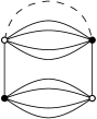
Figure 2: Typical contribution to the 2-points observable. The dashed line represents the contraction with the propagator $\partial_{k}R_{k}$.

The operator $F_{k(1)}$ is a sum over the intermediate colors labeling each 4-valent bubbles: $F_{k(1)}=\sum_{i=1}^{5}F_{k(1)}^{(i)}$, and each term contribute separately to the wave function and mass flow. As a result, we focus our attention on the computation of the trace for the case $i=1$. As explained in [41], we will identify the contribution to the coupling of a given bubble in the l.h.s by expanding the r.h.s around its local approximation i.e. around the value $q=0$, where $q$ denote the ”external momentum” shared by the red lines in the Figure (2). The two-points case is in a sense the more interesting, because for the wave function contribution, the local expansion require the first deviation to the exact local approximation, corresponding to the mass-term. This first deviation is proportional to $q^{2}$. Then, identifying the terms in front of each powers of $q^{2}$, we find:

$$k\partial_{k}m^{2}(k)=-5\lambda_{1}(k)\frac{k\partial_{k}Z(k)(S_{1}(0)k^{2}-S_{2}(0))+2Z(k)k^{2}S_{1}(0)}{[Z(k)k^{2}+m^{2}(k)]^{2}}$$ (33)

$$k\partial_{k}Z(k)=\frac{-2\lambda_{1}(k)Z(k)k^{2}S_{1}^{{}^{\prime\prime}}}{[Z(k)k^{2}+m^{2}(k)]^{2}+\lambda_{1}(k)(S_{1}^{{}^{\prime\prime}}k^{2}-S_{2}^{{}^{\prime\prime}})}$$ (34)

where the factor $5$ in front of the equation (33) takes into account the contributions for each $i$, $S_{l}^{{}^{\prime\prime}}$ denote the coefficient in front of $q^{2}$ in the expansion of $S_{i}(q)$ in power of $q$, and the sums $S_{1}$ and $S_{2}$ are :

$$S_{1}(q)=\sum_{\vec{p}\in\mathbb{Z}^{4}}\delta\bigg{(}\sum_{i=1}^{4}p_{i}+q\bigg{)}\theta(k^{2}-q^{2}-\vec{p}^{\,2}),$$ (35)

$$S_{2}(q)=\sum_{\vec{p}\in\mathbb{Z}^{4}}\vec{p}^{\,2}\delta\bigg{(}\sum_{i=1}^{4}p_{i}+q\bigg{)}\theta(k^{2}-q^{2}-\vec{p}\,^{2}).$$ (36)

Since we will be mostly interested in the large-$k$ limit, we can approximate the sums by integrals, replacing the Kronecker deltas by Dirac deltas. The support of the integrals is in the intersection of the hyperplane of equation $q+\sum_{l=1}^{4}p_{l}=0$ and the $4$-ball of radius $\sqrt{k^{2}-q^{2}}$. Note that the Kronecker delta of the closure constraint can be rewritten as $q+\vec{p}\cdot\vec{n}=0$, where $\vec{n}=(1,1,1,1)\in\mathbb{R}^{4}$ is the vector with all components equals to $1$. Using the rotational invariance of our integral, we can choose one of our coordinate axis to be in the direction $\vec{n}$. If we choose the axis $1$ in this direction, our constraint writes as $\delta(q+p^{\prime}_{1}|\vec{n}|)=\delta(q+2p^{\prime}_{1})=\delta(q/2+p^{\prime}_{1})/2$, and we find the following integral approximation:

$$S_{1}(q) \simeq \frac{1}{2}\Omega_{3}\bigg{[}k^{2}-\frac{5q^{2}}{4}\bigg{]}^{\frac{3}{2}}$$ (37)

$$S_{2}(q) \simeq \frac{1}{2}\Big{[}\frac{5q^{2}}{4}+\frac{3}{5}\bigg{(}k^{2}-\frac{5q^{2}}{4}\bigg{)}\Big{]}\Omega_{3}\bigg{(}k^{2}-\frac{5q^{2}}{4}\bigg{)}^{\frac{3}{2}},$$ (38)

where $\Omega_{d}:=\pi^{d/2}/\Gamma(d/2+1)$ is the volume of the unit $d$-ball, with the special value $\Omega_{3}=4\pi/3$. Using this integral approximation, we obtain:

$$S_{1}(0)=\frac{2}{3}\pi k^{3},\quad S_{2}(0)=\frac{2}{5}\pi k^{5},\quad S_{1}^{{}^{\prime\prime}}=-\frac{5}{4}\pi k,\quad S_{2}^{{}^{\prime\prime}}=-\frac{5}{12}\pi k^{3}$$ (39)

giving:

$$k\partial_{k}m^{2}(k)=-\frac{4\pi}{3}\lambda_{1}(k)\frac{\eta(k)+5}{[Z(k)k^{2}+m^{2}(k)]^{2}}k^{5}$$ (40)

$$\eta(k)=\frac{5\pi}{2}\lambda_{1}(k)\frac{k^{3}}{[Z(k)k^{2}+m^{2}(k)]^{2}-\lambda_{1}(k)\frac{5}{6}\pi k^{3}}$$ (41)

with the anomalous dimension $\eta(k)$ defined as:

$$\eta(k):=k\partial_{k}\ln(Z(k)).$$ (42)

Note that, in this case, and for the other computations, the extraction of the local approximation in the UV limit brings up a very nice property of the melonic sector, called   traciality. Traciality is a concept firstly introduced in a perturbative renormalization framework, ensuring that local approximation of high subgraphs make sense in the TFGT context [23], [25].

3.2.2 Flow equation for $\lambda_{1}$

The flow equation for $\lambda_{1}$ (29) involves two traces that we will compute separately. The first trace $\mathrm{Tr}_{GI}\big{[}\partial_{k}R_{k}\mathcal{K}_{k}^{-1}F_{k,(2)}\mathcal{K}_{k}^{-1}\big{]}$ involves two typical contributions that we have pictured in Figure (3) below. Note that the two diagrams pictured on this Figure have the same connectivity as the 4-valent interaction with intermediate line of color red, and we will only consider the flow equation for the coupling attached to one of the five color.

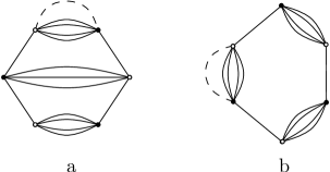
Figure 3: Contributions coming from the 6-points interactions to the 4-point interaction.

The computation of these two contributions follows exactly the same way as the extraction of the flow equation for the mass parameter. We expand with respect to the external momentum $q$ (i.e. the momentum around the external face sharing the same line as the four internal faces) around $q=0$, the first term of the expansion giving the relevant contribution. Because the two sums involve a loop of length one, they can be expressed in terms of the two sums $S_{1}$ and $S_{2}$, and we find:

$$\mathrm{Tr}_{GI}\big{[}k\partial_{k}R_{k}\mathcal{K}_{k}^{-1}F_{k,(2)\eqref{fig3}a}\mathcal{K}_{k}^{-1}\big{]}= 4\lambda_{3}\frac{k\partial_{k}Z(k)(S_{1}(0)k^{2}-S_{2}(0))+2Z(k)k^{2}S_{1}(0)}{[Z(k)k^{2}+m^{2}(k)]^{2}}$$ (43)

$$\times\sum_{\{\vec{p}_{i}\}\,i=1,...,4}\mathcal{W}^{(\ell)}_{\vec{p}_{1},\vec{p}_{2},\vec{p}_{3},\vec{p}_{4}}T_{\vec{p}_{1}}\bar{T}_{\vec{p}_{2}}T_{\vec{p}_{3}}\bar{T}_{\vec{p}_{4}}+\mathcal{O}(q),$$

$$\mathrm{Tr}_{GI}\big{[}k\partial_{k}R_{k}\mathcal{K}_{k}^{-1}F_{k,(2)\eqref{fig3}b}\mathcal{K}_{k}^{-1}\big{]}= \lambda_{2}\frac{k\partial_{k}Z(k)(S_{1}(0)k^{2}-S_{2}(0))+2Z(k)k^{2}S_{1}(0)}{[Z(k)k^{2}+m^{2}(k)]^{2}}$$ (44)

$$\times\sum_{\{\vec{p}_{i}\}\,i=1,...,4}\mathcal{W}^{(\ell)}_{\vec{p}_{1},\vec{p}_{2},\vec{p}_{3},\vec{p}_{4}}T_{\vec{p}_{1}}\bar{T}_{\vec{p}_{2}}T_{\vec{p}_{3}}\bar{T}_{\vec{p}_{4}}+\mathcal{O}(q).$$

The contribution of the last trace $\mathrm{Tr}_{GI}\big{[}\partial_{k}R_{k}\mathcal{K}_{k}^{-1}(F_{k,(1)}\mathcal{K}_{k}^{-1})^{2}\big{]}$ is graphically pictured in Figure (4), where the dotted line means contraction with Kronecker delta.

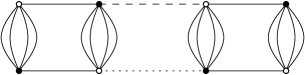
Figure 4: Contribution to the 4-point interaction involved two vertices.

Expanding in local approximation, we find, for the extra-local contribution with $q=0$:

$$\mathrm{Tr}_{GI}\big{[}k\partial_{k}R_{k}\mathcal{K}_{k}^{-1}(F_{k,(1),\eqref{fig4}}\mathcal{K}_{k}^{-1})^{2}\big{]} \approx \lambda_{1}^{2}(k)\frac{k\partial_{k}Z(k)(S_{1}(0)k^{2}-S_{2}(0))+2Z(k)k^{2}S_{1}(0)}{[Z(k)k^{2}+m^{2}(k)]^{3}}$$ (45)

$$\times \sum_{\{\vec{p}_{i}\}\,i=1,...,4}\mathcal{W}^{(\ell)}_{\vec{p}_{1},\vec{p}_{2},\vec{p}_{3},\vec{p}_{4}}T_{\vec{p}_{1}}\bar{T}_{\vec{p}_{2}}T_{\vec{p}_{3}}\bar{T}_{\vec{p}_{4}}.$$ (46)

Hence, summing the contributions (43), (44) and (45), and using the integral approximation for the sums, we find:

$$k\partial_{k}\lambda_{1}(k)=-(\lambda_{2}+4\lambda_{3})\frac{4\pi}{15}\frac{\eta(k)+5}{[Z(k)k^{2}+m^{2}(k)]^{2}}k^{5}+\lambda_{1}^{2}(k)\frac{4\pi}{15}\frac{\eta(k)+5}{[Z(k)k^{2}+m^{2}(k)]^{3}}k^{5}$$ (47)

3.2.3 Flow equations for $\lambda_{2}$ and $\lambda_{3}$

The only contribution to $\lambda_{3}$ is pictured in Figure (5) below, corresponding to the trace:

$$\mathrm{Tr}_{GI}\big{[}\partial_{k}R_{k}\mathcal{K}_{k}^{-1}F_{k,(1)}\mathcal{K}_{k}^{-1}F_{k,(2)}\mathcal{K}_{k}^{-1}\big{]}.$$

Indeed, it is the only contraction in the melonic sector with the same connectivity as the 6-point interaction associated with the coupling $\lambda_{3}$.

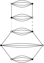
Figure 5: Contribution to the flow of $\lambda_{3}$

The local approximation of the diagram can be computed exactly as for the contribution (3) to $\lambda_{1}$, and we obtain:

$$\mathrm{Tr}_{fig\,\eqref{fig5}}(q=0) = \lambda_{1}\lambda_{3}\frac{k\partial_{k}Z(k)(S_{1}(0)k^{2}-S_{2}(0))+2Z(k)k^{2}S_{1}(0)}{[Z(k)k^{2}+m^{2}(k)]^{3}}$$ (49)

$$\times\sum_{\{\vec{p}_{i}\}\,i=1,...,6}\mathcal{Y}^{(\ell)}_{\vec{p}_{1},\vec{p}_{2},\vec{p}_{3},\vec{p}_{4},\vec{p}_{5},\vec{p}_{6}}T_{\vec{p}_{1}}\bar{T}_{\vec{p}_{2}}T_{\vec{p}_{3}}\bar{T}_{\vec{p}_{4}}T_{\vec{p}_{5}}\bar{T}_{\vec{p}_{6}}$$

and:

$$k\partial_{k}\lambda_{3}(k)=\frac{16\pi}{15}\lambda_{1}\lambda_{3}\frac{\eta(k)+5}{[Z(k)k^{2}+m^{2}(k)]^{3}}k^{5}.$$ (50)

In the same way, the contribution to the local approximation of the diagram (6)a to the flow equation for $\lambda_{2}$ writes as:

$$\mathrm{Tr}_{fig\,\eqref{fig6}a}(q=0) = \lambda_{1}\lambda_{2}\frac{k\partial_{k}Z(k)(S_{1}(0)k^{2}-S_{2}(0))+2Z(k)k^{2}S_{1}(0)}{[Z(k)k^{2}+m^{2}(k)]^{3}}$$ (52)

$$\times\sum_{\{\vec{p}_{i}\}\,i=1,...,6}\mathcal{X}^{(\ell)}_{\vec{p}_{1},\vec{p}_{2},\vec{p}_{3},\vec{p}_{4},\vec{p}_{5},\vec{p}_{6}}T_{\vec{p}_{1}}\bar{T}_{\vec{p}_{2}}T_{\vec{p}_{3}}\bar{T}_{\vec{p}_{4}}T_{\vec{p}_{5}}\bar{T}_{\vec{p}_{6}}$$

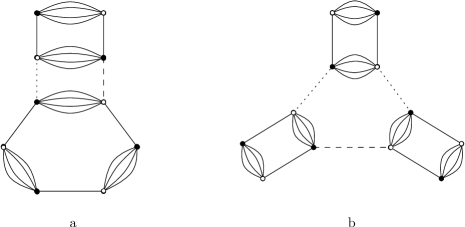
Figure 6: Contribution to the flow of $\lambda_{2}$

Finally, the contribution coming from the diagram (6)b in Figure (6) involves a loop with two delta propagators, and:

$$\mathrm{Tr}_{fig\,\eqref{fig6}b}(q=0) = \lambda_{1}^{3}(k)\frac{k\partial_{k}Z(k)(S_{1}(0)k^{2}-S_{2}(0))+2Z(k)k^{2}S_{1}(0)}{[Z(k)k^{2}+m^{2}(k)]^{4}}$$ (54)

$$\times\sum_{\{\vec{p}_{i}\}\,i=1,...,6}\mathcal{X}^{(\ell)}_{\vec{p}_{1},\vec{p}_{2},\vec{p}_{3},\vec{p}_{4},\vec{p}_{5},\vec{p}_{6}}T_{\vec{p}_{1}}\bar{T}_{\vec{p}_{2}}T_{\vec{p}_{3}}\bar{T}_{\vec{p}_{4}}T_{\vec{p}_{5}}\bar{T}_{\vec{p}_{6}}.$$

Grouping together the contributions (52) and (54), we find:

$$k\partial\lambda_{2}=\frac{24\pi}{15}\lambda_{1}\lambda_{2}\frac{\eta(k)+5}{[Z(k)k^{2}+m^{2}(k)]^{3}}k^{5}-\frac{12\pi}{15}\lambda_{1}^{3}\frac{\eta(k)+5}{[Z(k)k^{2}+m^{2}(k)]^{4}}k^{5}.$$ (55)

3.2.4 Dimensionless renormalized parameters

Taking into account the canonical dimension define in Section (2.2), the renormalized dimensionless couplings are defined as:

$$m=\sqrt{Z}k\bar{m}\qquad{\lambda}_{1}=Z^{2}k\bar{\lambda}_{1}\qquad\lambda_{2}=Z^{3}\bar{\lambda}_{2}\qquad\lambda_{3}=Z^{3}\bar{\lambda}_{3}$$ (56)

Using the flow equations (41), (40), (47), (55) and (50), we find for the dimensionless renormalized couplings the following autonomous system:

$$\eta(k)=\frac{5\pi}{2}\bar{\lambda}_{1}(k)\frac{1}{[1+\bar{m}^{2}(k)]^{2}-\bar{\lambda}_{1}(k)\frac{5}{6}\pi}$$ (57)

$$\beta_{m^{2}}=-(2+\eta)\bar{m}^{2}(k)-\frac{4\pi}{3}\bar{\lambda}_{1}(k)\frac{\eta(k)+5}{[1+\bar{m}^{2}(k)]^{2}}$$ (58)

$$\beta_{\lambda_{1}}=-(1+2\eta)\bar{\lambda}_{1}(k)-(\bar{\lambda}_{2}+4\bar{\lambda}_{3})\frac{4\pi}{15}\frac{\eta(k)+5}{[1+\bar{m}^{2}(k)]^{2}}+\bar{\lambda}_{1}^{2}(k)\frac{4\pi}{15}\frac{\eta(k)+5}{[1+\bar{m}^{2}(k)]^{3}}$$ (59)

$$\beta_{\lambda_{3}}=-3\eta\bar{\lambda}_{3}(k)+\frac{16\pi}{15}\bar{\lambda}_{1}\bar{\lambda}_{3}\frac{\eta(k)+5}{[1+\bar{m}^{2}(k)]^{3}}.$$ (60)

$$\beta_{\lambda_{2}}=-3\eta\bar{\lambda}_{2}(k)+\frac{24\pi}{15}\bar{\lambda}_{1}\bar{\lambda}_{2}\frac{\eta(k)+5}{[1+\bar{m}^{2}(k)]^{3}}-\bar{\lambda}_{1}^{3}\frac{12\pi}{15}\frac{\eta(k)+5}{[1+\bar{m}^{2}(k)]^{4}}\,,$$ (61)

with the definition : $\beta_{i}:=k\partial_{k}\bar{i}$, $i\in\{m^{2},\lambda_{1},\lambda_{2},\lambda_{3}\}$.

4 Fixed points in the UV regime

At vanishing $\beta$-functions we obtain a fixed points. But these fixed points does not get any quantum correction and is called the Gaussian fixed point. In the neighborhood of these fixed points, the stability is determined by the linearized system of $\beta$-functions. All these points are studied in detail in this section.

4.1 Vicinity of the Gaussian fixed point

The autonomous system describing the flow of the dimensionless couplings admits a trivial fixed point for the values $\bar{\lambda}_{1}=\bar{\lambda}_{2}=\bar{\lambda}_{3}=\bar{m}=0$ called Gaussian Fixed Point (GFP). Expanding our equations around this points, we find the reduced autonomous system:

$$\begin{cases}\phantom{-}\beta_{m^{2}}&\approx-2\bar{m}^{2}-\frac{20\pi\bar{\lambda}_{1}}{3}\,,\\ \phantom{-}\beta_{\lambda_{1}}&\approx-\bar{\lambda}_{1}-\frac{4\pi}{3}(\bar{\lambda}_{2}+4\bar{\lambda}_{3})\big{(}1+\frac{\pi}{2}\bar{\lambda}_{1}+2\bar{m}^{2}\big{)}-\frac{11\pi}{3}\bar{\lambda}_{1}^{2}\,,\\ \phantom{-}\beta_{\lambda_{2}}&\approx\frac{\pi}{2}\bar{\lambda}_{1}\bar{\lambda}_{2}\,,\\ \phantom{-}\beta_{\lambda_{3}}&\approx-\frac{13\pi}{6}\bar{\lambda}_{1}\bar{\lambda}_{3}\end{cases}$$ (62)

and the anomalous dimension:

$$\eta(k)\approx\frac{5\pi\bar{\lambda}_{1}}{2}\,.$$ (63)

These equations give the qualitative behavior of the RG trajectories around the GFP. In order to study its stability, we compute the   stability matrix $\beta_{ij}:=\partial_{i}\beta_{j}\,i\in\{m^{2},\lambda_{1},\lambda_{2},\lambda_{3}\}$, and evaluate each coefficient at the GFP. We find:

$$\beta^{GFP}_{ij}:=\begin{pmatrix}-2&0&0&0\\ -\frac{20\pi}{3}&-1&0&0\\ 0&-\frac{4\pi}{3}&0&0\\ 0&-\frac{16\pi}{3}&0&0\end{pmatrix},$$ (64)

with eigenvalues $(-2,-1,0,0)$ and eigenvectors $e_{1}^{GFP}=(\frac{9}{160\pi^{2}},\frac{3}{8\pi},\frac{1}{4},1);\,$ $e_{2}^{GFP}=(0,\frac{3}{16\pi},\frac{1}{4},1);\,$ $e_{3}^{GFP}=(0,0,0,1);\,$ $e_{4}^{GFP}=(0,0,1,0)$. One recall that the   critical exponents are the opposite values of the eigenvalues of the $\beta_{ij}$, and that the fixed point can be classified following the sign of their critical exponents. Hence, we have two relevant directions in the UV, with critical exponents $2$ and $1$, and two marginal couplings with zero critical exponents. Moreover, note that the critical exponents are equal to the canonical dimension around the GFP. Finally, note that the previous system of equations admits other fixed points, or a   line of fixed points in addition to the Gaussian one, for the values: $\bar{\lambda}_{1}=\bar{m}=0$; $\bar{\lambda}_{3}=-\bar{\lambda}_{2}/4$. This fixed point occurs as well as in the non-perturbation analysis, and we will return on this subject in the next Section.

For the moment, we are in position to discuss the qualitative flow diagram around the Gaussian fixed point. First of all, note that all the coefficients of the beta function of the system (62) are not negative definite. This fact seems to be a special feature of this model, meaning that the weight of the anomalous dimension does not dominate the vertex contribution. This fact is a first difference with respect to the similar non-Abelian $\phi^{6}$ model studied in [37]. However, the analysis providing in this reference remains true, and the model is not asymptotically free. We will not repeat the complete analysis given in [37] , but a qualitative argument is the following. Exploiting the fact that the hyperplans $\bar{\lambda}_{2}=0$ and $\bar{\lambda}_{3}=0$ are invariant under the flow, we can look at only a two-dimensional reduction of the complete system (62). We choose $\bar{\lambda}_{2}=0$, and plot the numerical integration of the reduced flow equation in Figure (7) (on the left) below.

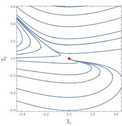
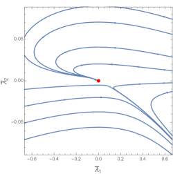
Figure 7: Phase portrait in the plans $(\bar{\lambda}_{1},\bar{\lambda}_{3})$ for $\bar{\lambda}_{2}=0$ (one the left) and in the plan $(\bar{\lambda}_{1},\bar{\lambda}_{2})$, for $\bar{\lambda}_{3}=0$.

In the domain, $\bar{\lambda}_{3}>0$, even if a given trajectory approaches of the Gaussian fixed point, $\bar{\lambda}_{1}$ reaches a negative value, and it is ultimately repelled for $k$ sufficiently large. The same phenomenon occurs for $\bar{\lambda_{2}}$ in the plan $\bar{\lambda}_{2}<0$ (see the Figure(7) one the right). The issue of the UV completion of a theory which is non-Asymptotically free is one of the difficult question that we address to the non-perturbative renormalization group machinery, and the rest of this paper is essentially devoted to this one.

4.2 Non-Gaussian fixed points

Solving numerically the systems (40)-(50), we find some non-Gaussian fixed points, whose relevant characteristics are summarized in the Table (1) below. In addition to these non-Gaussian fixed points, the system admits a   line of fixed points, $LFP$, for the values:

$$LFP=\{\bar{m}^{2}=0,\bar{\lambda}_{1}=0,\bar{\lambda}_{2}=-4\bar{\lambda}_{3}\}\,,$$ (65)

with critical exponents:

$$\begin{cases}\phantom{-}\theta^{(1)}&=-2\,,\\ \phantom{-}\theta^{(2)}&=\,\,\,\,\,0\,,\\ \phantom{-}\theta^{(3)}&=-\frac{1}{2}\big{(}1+\sqrt{1-\frac{128}{9}\pi^{2}\bar{\lambda}_{2}}\big{)}\,,\\ \phantom{-}\beta_{\lambda_{3}}&=-\frac{1}{2}\big{(}1-\sqrt{1-\frac{128}{9}\pi^{2}\bar{\lambda}_{2}}\big{)}.\end{cases}$$ (66)

FP	$\bar{m}^{2}$	$\bar{\lambda}_{1}$	$\bar{\lambda}_{2}$	$\bar{\lambda}_{3}$	$\eta$	$\theta^{(1)}$	$\theta^{(2)}$	$\theta^{(3)}$	$\theta^{(4)}$
$FP_{1}$	-0.3	0.005	0.0009	-0.0002	-6.3	-299	56.1	-11.7	5.8
$FP_{2}$	-0.7	0.008	0.0006	-0.0002	0.76	-7.4-1.9i	-7.4+1.9i	3.34	-0.12
$FP_{3}$	-0.9	0.0007	3.32.$10^{-6}$	0.	1.3	-66.7	-42.63	-27.7	1.80
$FP_{4}$	-0.8	0.04	-0.02	0.	-5.9	-144.8	-14.4	-7.5	-5.4
$FP_{5}$	0.06	-0.006	0.002	0.	-0.04	1.9	1.09	-0.04	-0.01
$FP_{6}$	1.32	-0.5	-0.06	0.	-0.6	3.0	-1.23	-1.13	-0.39

Table 1: Summary of the properties of the non-Gaussian fixed points. Again, the critical exponents $\theta^{i}$ are the opposite values of the eigenvalues of the stability matrix: $\beta_{*}=:\mathrm{diag}(-\theta^{1}_{*},-\theta^{2}_{*},-\theta^{3}_{*},-\theta^{4}_{*})$.

The denominator of $\eta$, $D:=[1+\bar{m}^{2}(k)]^{2}-\bar{\lambda}_{1}(k)\frac{5}{6}\pi$ introduce a singularity in the flow. At the Gaussian fixed point, and in a sufficiently small domain around, $D>0$. But further away from the GFP, $D$ may cancel, creating in the $(\bar{\lambda}_{1},\bar{m}^{2})$-plan a singularity line. The area below this line where $D<0$ is thus disconnected from the region $D>0$ connected to GFP. Then, we ignore for our purpose the fixed points in the disconnected region, for which $D<0$. A direct computation show that only the fixed points $FP_{2}$, $FP_{3}$, $FP_{5}$ and $FP_{6}$ are relevant for an analysis in the domain connected to the Gaussian fixed point.

$\bullet$ The fixed points $FP_{2}$ and $FP_{3}$ are very similar. They have three irrelevant directions and one relevant direction in the UV. For each of these fixed points, the three irrelevant directions span a three dimensional manifold on which the trajectory runs toward the fixed point in the IR, while the trajectories out side are repelled of this critical surface, as pictured on Figure (8). This picture, the existence of a separatrix between two connected regions of the phase space is reminiscent of a critical behavior, with phase transition between a broken and a symmetric phase, and these separatrix are   IR-critical surfaces. This interpretation is highlighted for the two fixed points in the zero momenta limit. Indeed, in both cases, the contributions in the effective action of the terms proportionals to $\bar{\lambda}_{2}$ and $\bar{\lambda}_{3}$ can be neglected in comparison with the contributions of the two first terms, leading in the first approximation a Ginsburg-Landau equation for $\phi^{4}$ scalar complex theory. Note that for $FP_{2}$ two critical exponents are complex, providing some oscillations of the trajectories, and implying that the fixed point is an IR-attractor in the two-dimensional manifold spanned by the eigenvectors corresponding to these two critical exponents. Moreover, the fixed point $FP_{6}$ appears to be an IR fixed point, with coordinates of opposite sign.

$\bullet$ The fixed point $FP_{5}$ has two relevant and two irrelevant directions in the UV. The relevant directions in the UV span a two-dimensional manifold corresponding to a   UV-multicritical surface. Such a surface is interesting for the UV-completion of the theory. Indeed, all the trajectories in the surface are oriented toward the fixed point in the UV, while the dimension of the surface give an interesting number of physical parameter, providing an evidence in favor of the   asymptotic safety of the model in the UV [52].

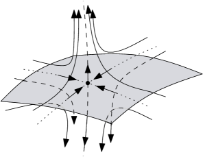
Figure 8: Qualitative behavior of the RG trajectories around an IR fixed point. The critical surface is spanned by the relevant directions in the IR, and the arrows are oriented toward the IR direction. This illustrates the senario of asymptotically safety.

$\bullet$ Finally, we have the line of fixed point, for which we will distinguish four cases:

i   In the domain $d_{1}=\{\bar{\lambda}_{2}<0\}$ we have two relevant, one marginal and one irrelevant directions.

ii   At the point $d_{2}=\{\bar{\lambda}_{2}=0\}$, we recover the GFP, with two relevant and two marginal directions.

iii   In the domain $d_{3}=\{\bar{\lambda}_{2}\in]0,\big{(}\frac{3}{8\pi}\big{)}^{2}]\,\}$ we have three relevant and one marginal directions. One more time, this section of the critical line is interesting in view of the UV-completion of the theory and provide a supplementary evidence if favor of asymptotic safety. Indeed, in each points, the relevant directions in the UV span a three dimensional UV-critical surface, in favor of the existence of a non-trivial asymptotically safe theory with three independent physical parameters. This line of fixed point has been recently discussed in [43] for a similar model improved by unconnected interaction bubbles.

iv   In the domain $d_{4}=\{\bar{\lambda}_{2}>\big{(}\frac{3}{8\pi}\big{)}^{2}\,\}$ The situation is very reminiscent of the previous one. We have three eigenvalues with negative real part and one equal to zero. Hence, we have three relevant and one marginal directions. The only difference in comparison with the domain $d_{3}$ is that the eigenvalue have non-zero imaginary parts, giving some oscillations and attractor phenomena in the trajectories.

Finally, we briefly discuss the values of the anomalous dimensions. With our conventions, the couplings of the relevant operator are suppressed as a power of $k$ in the UV limit $k\rightarrow\infty$. The couplings decrease when the trajectory goes away from the UV regime. However, the power law behavior is limited to the attractive region of the fixed point, far from its scaling regime it can deviate from the power law one. And we can evaluate this deviation. For instance, in the vicinity of $FP_{5}$, one deduce from (24) that the canonical dimension becomes:

$$[t_{b}]_{FP_{5}}\approx 3-1.6\frac{N_{b}}{2}\,,$$ (67)

from which we deduce that all the interaction of valence up or equal to four becomes inessentials. The same phenomenon occurs in the vicinity of $FP_{4}$, where all the interactions up to these of valence four become inessentials. In contrary, at the fixed points $FP_{2}$ and $FP_{4}$ the anomalous dimension is positive, meaning that the power counting is improved with respect to the Gaussian one, and irrelevent operators are enhanced in the UV.

5 Truncation with an interaction of valence 8

This section aims to identify how the adding of interaction of the valence $8$ may modify the flow equation and the fixed point of our model. This means that the effective action is now truncate to satisfy the following form: let $e_{ji}\in[1,5]$ is the color of the bubble of valence 8, with $i=1,2,3,4$ and $j=1,2,\cdots,5,$

$$\Gamma_{k}[\bar{T},T] = \sum_{\vec{p}\in\mathbb{Z}^{5}}\bigg{(}Z(k)\vec{p}\,^{2}+m^{2}(k)\bigg{)}\bar{T}_{\vec{p}}T_{\vec{p}}+\frac{\lambda_{1}(k)}{2}\sum_{\ell=1}^{5}\sum_{\{\vec{p}_{i}\}\,i=1,...,4}\mathcal{W}^{(\ell)}_{\vec{p}_{1},\vec{p}_{2},\vec{p}_{3},\vec{p}_{4}}T_{\vec{p}_{1}}\bar{T}_{\vec{p}_{2}}T_{\vec{p}_{3}}\bar{T}_{\vec{p}_{4}}+$$ (68)

$$+ \frac{\lambda_{2}(k)}{3}\sum_{\ell=1}^{5}\sum_{\{\vec{p}_{i}\}\,i=1,...,6}\mathcal{X}^{(\ell)}_{\vec{p}_{1},\vec{p}_{2},\vec{p}_{3},\vec{p}_{4},\vec{p}_{5},\vec{p}_{6}}T_{\vec{p}_{1}}\bar{T}_{\vec{p}_{2}}T_{\vec{p}_{3}}\bar{T}_{\vec{p}_{4}}T_{\vec{p}_{5}}\bar{T}_{\vec{p}_{6}}$$ (69)

$$+ \lambda_{3}(k)\sum_{\ell_{i}=1,i=1,2,3}^{5}\sum_{\{\vec{p}_{i}\}\,i=1,...,6}\mathcal{Y}^{(\ell_{1},\ell_{2},\ell_{3})}_{\vec{p}_{1},\vec{p}_{2},\vec{p}_{3},\vec{p}_{4},\vec{p}_{5},\vec{p}_{6}}T_{\vec{p}_{1}}\bar{T}_{\vec{p}_{2}}T_{\vec{p}_{3}}\bar{T}_{\vec{p}_{4}}T_{\vec{p}_{5}}\bar{T}_{\vec{p}_{6}}$$ (70)

$$+ \sum_{i=1}^{4}\lambda_{4,i}(k)\sum_{e_{ji}=1/,e_{ji}\neq e_{ki}\forall j\neq k}^{5}\sum_{\{\vec{p}_{l}\}\,l=1,...,8}\mathcal{Z}^{i,(e_{ji})}_{\vec{p}_{1},\vec{p}_{2},\vec{p}_{3},\vec{p}_{4},\vec{p}_{5},\vec{p}_{6},\vec{p}_{7},\vec{p}_{8}}T_{\vec{p}_{1}}\bar{T}_{\vec{p}_{2}}T_{\vec{p}_{3}}\bar{T}_{\vec{p}_{4}}T_{\vec{p}_{5}}\bar{T}_{\vec{p}_{6}}T_{\vec{p}_{7}}\bar{T}_{\vec{p}_{8}},$$ (71)

where we assume that the last term of the action (68) takes into account all contributions of melonic interactions of the form $T^{8}$, and the coupling constants $\lambda_{4,i},\,\,i=1,2,3,4$ are related to the vertex $V_{4,i}$ see figures (9). The set $\{e_{\cdot\,i}\}_{j}$ takes into account all the colors associated to the vertices $V_{4,i}$.

$V_{4,1}$           $V_{4,2}$       $V_{4,3}$          $V_{4,4}$

Figure 9: Graphical representation of the vertices of valence 8

We get for $\Gamma_{k,(3)}$ and $\Gamma_{k,(4)}$ the flow equations:

$$k\partial_{k}\Gamma_{k,(3)} = 2\mathrm{Tr}_{GI}\big{[}\partial_{k}R_{k}\mathcal{K}_{k}^{-1}F_{k,(1)}\mathcal{K}_{k}^{-1}F_{k,(2)}\mathcal{K}_{k}^{-1}\big{]}-\mathrm{Tr}_{GI}\big{[}\partial_{k}R_{k}\mathcal{K}_{k}^{-1}(F_{k,(1)}\mathcal{K}_{k}^{-1})^{3}\big{]}$$ (73)

$$-\mathrm{Tr}_{GI}\big{[}\partial_{k}R_{k}\mathcal{K}_{k}^{-1}F_{k,(3)}\mathcal{K}_{k}^{-1}\big{]}\,,$$

and

$$k\partial_{k}\Gamma_{k,(4)} = -\mathrm{Tr}_{GI}\big{[}\partial_{k}R_{k}\mathcal{K}_{k}^{-1}F_{k,(4)}\mathcal{K}_{k}^{-1}\big{]}+\mathrm{Tr}_{GI}\big{[}\partial_{k}R_{k}\mathcal{K}_{k}^{-1}(F_{k,(2)}\mathcal{K}_{k}^{-1})^{2}\big{]}$$ (76)

$$+\mathrm{Tr}_{GI}\big{[}\partial_{k}R_{k}\mathcal{K}_{k}^{-1}(F_{k,(1)}\mathcal{K}_{k}^{-1})^{4}\big{]}$$

$$-3\mathrm{Tr}_{GI}\big{[}\partial_{k}R_{k}\mathcal{K}_{k}^{-1}F_{k,(2)}\mathcal{K}_{k}^{-1}(F_{k,(1)}\mathcal{K}_{k}^{-1})^{2}\big{]},$$

Taking into account the dimensionless renormalized parameter, and grouping all melonic contributions, the flow equations of the coupling constants $\bar{\lambda}_{2}$, $\bar{\lambda}_{3}$ and $\bar{\lambda}_{4,i}$, are:

$$\begin{cases}\phantom{-}\beta_{m^{2}}&=-(2+\eta)\bar{m}^{2}-\frac{4\pi}{3}\bar{\lambda}_{1}\frac{\eta+5}{[1+\bar{m}^{2}]^{2}}\,,\\ \phantom{-}\beta_{\lambda_{1}}&=-(1+2\eta)\bar{\lambda}_{1}-(\bar{\lambda}_{2}+4\bar{\lambda}_{3})\frac{4\pi}{15}\frac{\eta+5}{[1+\bar{m}^{2}]^{2}}+\bar{\lambda}_{1}^{2}\frac{4\pi}{15}\frac{\eta+5}{[1+\bar{m}^{2}]^{3}}\,,\\ \phantom{-}\beta_{\lambda_{2}}&=-3\eta\bar{\lambda}_{2}+\frac{24\pi}{15}\bar{\lambda}_{1}\bar{\lambda}_{2}\frac{\eta+5}{[1+\bar{m}^{2}]^{3}}-\bar{\lambda}_{1}^{3}\frac{12\pi}{15}\frac{\eta+5}{[1+\bar{m}^{2}]^{4}}-\frac{48\pi}{15}\bar{\lambda}_{4,2}\frac{\eta+5}{[1+\bar{m}^{2}]^{2}}-\frac{12\pi}{15}\bar{\lambda}_{4,4}\frac{\eta+5}{[1+\bar{m}^{2}]^{2}}\\ \phantom{-}\beta_{\lambda_{3}}&=-3\eta\bar{\lambda}_{3}+\frac{16\pi}{15}\bar{\lambda}_{1}\bar{\lambda}_{3}\frac{\eta+5}{[1+\bar{m}^{2}]^{3}}-\frac{8\pi}{15}\bar{\lambda}_{4,1}\frac{\eta+5}{[1+\bar{m}^{2}]^{2}}-\frac{36\pi}{15}\bar{\lambda}_{4,3}\frac{\eta+5}{[1+\bar{m}^{2}]^{2}}-\frac{8\pi}{15}\bar{\lambda}_{4,4}\frac{\eta+5}{[1+\bar{m}^{2}]^{2}}\,,\\ \phantom{-}\beta_{\lambda_{4,1}}&=(1-4\eta)\bar{\lambda}_{4,1}+\frac{16\pi}{15}\bar{\lambda}_{4,1}\bar{\lambda}_{1}\frac{\eta+5}{[1+\bar{m}^{2}]^{2}}+\frac{4\pi}{15}\bar{\lambda}_{3}^{2}\frac{\eta+5}{[1+\bar{m}^{2}]^{3}}-\frac{24\pi}{15}\bar{\lambda}_{1}^{2}\bar{\lambda}_{3}\frac{\eta+5}{[1+\bar{m}^{2}]^{4}}+\frac{4\pi}{15}\bar{\lambda}_{1}^{4}\frac{\eta+5}{[1+\bar{m}^{2}]^{5}}\,,\\ \phantom{-}\beta_{\lambda_{4,2}}&=(1-4\eta)\bar{\lambda}_{4,2}+\frac{32\pi}{15}\bar{\lambda}_{4,2}\bar{\lambda}_{1}\frac{\eta+5}{[1+\bar{m}^{2}]^{2}}+\frac{4\pi}{15}\bar{\lambda}_{2}^{2}\frac{\eta+5}{[1+\bar{m}^{2}]^{3}}-\frac{12\pi}{15}\bar{\lambda}_{1}^{2}\bar{\lambda}_{2}\frac{\eta+5}{[1+\bar{m}^{2}]^{4}}\,,\\ \phantom{-}\beta_{\lambda_{4,3}}&=(1-4\eta)\bar{\lambda}_{4,3}+\frac{24\pi}{15}\bar{\lambda}_{4,3}\bar{\lambda}_{1}\frac{\eta+5}{[1+\bar{m}^{2}]^{2}}\,,\\ \phantom{-}\beta_{\lambda_{4,4}}&=(1-4\eta)\bar{\lambda}_{4,4}+\frac{24\pi}{15}\bar{\lambda}_{4,4}\bar{\lambda}_{1}\frac{\eta+5}{[1+\bar{m}^{2}]^{2}}+\frac{8\pi}{15}\bar{\lambda}_{2}\bar{\lambda}_{3}\frac{\eta+5}{[1+\bar{m}^{2}]^{3}}-\frac{24\pi}{15}\bar{\lambda}_{1}^{2}\bar{\lambda}_{3}\frac{\eta+5}{[1+\bar{m}^{2}]^{4}}\end{cases}$$ (77)

with the anomalous dimension given by equation (57). One more time, the system can be solved numerically, and the fixed points as well as their essential properties are summarized in the Table (2).

FP	$FP_{1}$	$FP_{2}$	$FP_{3}$	$FP_{4}$	$FP_{5}$	$FP_{6}$	$FP_{7}$	$FP_{8}$	$FP_{9}$	$FP_{10}$
$\bar{m}^{2}$	-1.07	-0.91	-0.84	-0.84	-1.22	-0.75	-0.76	-0.74	-0.59	1.45
$\bar{\lambda}_{1}$	0.004	0.005	0.02	0.02	0.009	0.006	0.045	0.05	0.14	-0.65
$10^{2}\bar{\lambda}_{2}$	0.1	0.03	0.7	-0.4	0.2	-0.01	2	1	-40	-16
$10^{3}\bar{\lambda}_{3}$	-0.3	0.04	-3	0.	-0.7	0.02	-10	-10	-0.6	-3
$10^{2}\bar{\lambda}_{4,1}$	0.01	-0.04	0.1	0.01	0.001	-230	0.3	0.3	0.09	-0.3
$10^{3}\bar{\lambda}_{4,2}$	-0.04	-0.01	0.	-1	-0.06	-2000.	-0.9	-1	100	-10
$10^{3}\bar{\lambda}_{4,3}$	0.	0.	-0.3	-0.9	0.	0.	0.	0.	0.	0.
$10^{2}\bar{\lambda}_{4,4}$	0.003	690	0.02	0.4	0.006	670	0.05	0.2	0.03	-0.03
$\eta$	-6.8	-6.3	-6.0	-6.0	2.6	0.9	-5.9	-5.6	-0.65	-0.66
$\theta^{(1)}$	307.8	289.8	179.6	180.0	-110.7	24.7	142.6	137.9	121.6	3.2
$\theta^{(2)}$	-245.8	-112.0	-12+25i	-45.9	-50+13i	14.5	19+6i	20+4i	30	3.1
$\theta^{(3)}$	173.0	-67.8	-12-25i	31	-50-13i	12.2	19-6i	20-4i	23.6	-3.0
$\theta^{(4)}$	113.6	31+6.7i	21+10i	26	-39	7.7	11.7	13+1.7i	18.9	2.8
$\theta^{(5)}$	77+19i	31-6.6i	21-10i	-22	-33	-6	1.2+10i	13-1.7i	17.2	2.7
$\theta^{(6)}$	77-19i	-28.5	-15	10	24.8	5.7	1.2-10i	11	9.8	1.0
$\theta^{(7)}$	-67	-19	6	6.1	-18	-5	9.8	-5.7	6.3	0.7
$\theta^{(8)}$	7.2	5.8	2.2	4	-2.3	-1.3	5.5	5.4	5.2	0.3

Table 2: Summary of the properties of the non-Gaussian fixed points in the $\phi^{8}$ truncation.

Interestingly, note that the line of fixed points has disappeared, that is not a surprise, because such line of fixed points is generally a pathology of the crude truncation. Among the fixed points listed in the table, only $FP_{5}$, $FP_{6}$ and $FP_{10}$ have $D>0$. The over fixed points have a big critical exponent and become harmful pathology of the model.

$\bullet$ The fixed point $FP_{5}$ has seven irrelevant directions and one relevant direction in the UV, and seems to be an IR fixed point, whose irrelevant directions span an IR-critical surface with seven dimensions.

$\bullet$ The fixed point $FP_{6}$ has five relevant directions and three irrelevant directions in the UV. The relevant directions span an UV-multicritical surface of dimension five. The existence of a such sub-manifold is in accordance with the asymptotic safety of the theory.

$\bullet$ The fixed point $FP_{10}$ has seven relevant directions and one irrelevant direction in the UV. It correspond to an UV fixed point whose revelant directions span a seven-dimensional UV-critical surface. One more time, the existence of a such manifold seems to be in accordance with a non-trivial asymptotically safe theory.

At this stage, it is not obvious to make contact with the fixed points obtained in the previous truncation. The standard way to highlight these relation is to consider truncation with higher and higher valence, and seek convergence of the fixed points. But in our case, the difficulty of a such computations is very improved by the non-locality of the interactions, and these conclusions have to be confirmed by more finer analysis. Let us remark that the study of the critical exponent [49] could upset our analysis for the choice of the truncations with valances greater than $6$. For instance, the fixed point $FP_{5}$ leads to a very large critical exponent and this can help to show that the truncation in this order remains non consistent. For the fixed point $FP_{10}$ the critical exponent is small, and adding another interaction of valence more than 8 becomes unnecessary. Unlike, the fixed point $FP_{10}$ exhibits several relevant directions and these do not appear in the previous section by using just the truncation with interaction of valence $6$.

6 Discussion and conclusion

In this paper the renomalization group analysis is applied for just renormalizable $T^{6}_{5}$ TGFT model in the deep UV limit. Using the simplest approximation consisting in a truncation around the marginal interactions with respect to the perturbative power counting i.e. around the Gaussian fixed point, we have derived the flow equations for each couplings. Because we have focused our attention on the UV sector, the leading contributions to the flow equations provide to the melonic sector, a consideration which considerably simplify the computation of the flow equations. In a second time, using of the appropriate notion of canonical dimension in the UV, we have translated our flow equation in an autonomous system of differential equations, whose we have computed numerically the fixed points, as well as the behavior of the flow’s trajectory around each of them.

We have find two type of fixed points. The IR fixed points, whose relevant directions in the IR span an IR-critical surface, a picture in favor of phase-transitions. This is supported, for two of these IR fixed points, by the negative value of their mass-parameter, and the fact that in their vicinity, the effective action turn to be a Ginsburg-Landau like equation for a $\phi^{4}$ scalar complex theory, advocating a condensed phase transition interpretation. In opposition, the second type of fixed points are UV critical, and their relevant directions in the UV span critical surface with dimensions higher or equal to two, a picture in accordance with a well-defined and non-trivial behavior in the UV for asymptotically safe theories. In all the case, we observe that anomalous dimensions enhanced or weaken the UV-power counting for relevant operators with respect to the perturbative power-counting, a phenomena which seems to indicate a break-down of our crude truncation in these domains of the phase-space. Moreover, the presence of pathological effects as a line of fixed point seems to confirm these suspicions, as well as its disappearance in a higher-truncation, while our conclusions about asymptotic safety and IR fixed points remain true. The connection between the new fixed point and these ones obtained in the first truncation remains however unclear at this stage without more control over the approximation procedure.

Finally, note that in the complementary IR regime, the flow equations receive non-melonic contributions. This is due to the fact that, for a very small cut-off, the sums take values $0$ or $1$. As pointed in [41], the appropriate rescalling is provided by the standard power counting, and the flow equation turn as well to be an autonomous system, which can be solved numerically. However, we have to keep in mind that our model is defined on a compact manifold ($U(1)^{6}$ in the referenced paper, $U(1)^{5}$ in our case). Then, no phase transition can be occurs, and all the non-Gaussian fixed point reached to the Gaussian one when the cut-off tend to $0$, except if the radius of the circles tend simultaneously to the infinity.

References

- [1] R. Gurau and J. P. Ryan, “Colored Tensor Models - a review,” SIGMA 8, 020 (2012) doi:10.3842/SIGMA.2012.020 [arXiv:1109.4812 [hep-th]].
- [2] R. Gurau, “Colored Group Field Theory,” Commun. Math. Phys. 304, 69 (2011) doi:10.1007/s00220-011-1226-9 [arXiv:0907.2582 [hep-th]].
- [3] V. Rivasseau, “Constructive Tensor Field Theory,” arXiv:1603.07312 [math-ph].
- [4] V. Rivasseau, “Random Tensors and Quantum Gravity,” arXiv:1603.07278 [math-ph].
- [5] V. Rivasseau, “The Tensor Theory Space,” Fortsch. Phys. 62, 835 (2014) doi:10.1002/prop.201400057 [arXiv:1407.0284 [hep-th]].
- [6] V. Rivasseau, “The Tensor Track, III,” Fortsch. Phys. 62, 81 (2014) doi:10.1002/prop.201300032 [arXiv:1311.1461 [hep-th]].
- [7] V. Rivasseau, “The Tensor Track, IV,” arXiv:1604.07860 [hep-th].
- [8] V. Rivasseau, “The Tensor Track: an Update,” arXiv:1209.5284 [hep-th].
- [9] V. Bonzom, R. Gurau, J. P. Ryan and A. Tanasa, “The double scaling limit of random tensor models,” JHEP 1409, 051 (2014) doi:10.1007/JHEP09(2014)051 [arXiv:1404.7517 [hep-th]].
- [10] S. Dartois, R. Gurau and V. Rivasseau, “Double Scaling in Tensor Models with a Quartic Interaction,” JHEP 1309, 088 (2013) doi:10.1007/JHEP09(2013)088 [arXiv:1307.5281 [hep-th]].
- [11] T. Delepouve and R. Gurau, “Phase Transition in Tensor Models,” JHEP 1506, 178 (2015) doi:10.1007/JHEP06(2015)178 [arXiv:1504.05745 [hep-th]].
- [12] D. Benedetti and R. Gurau, “Symmetry breaking in tensor models,” Phys. Rev. D 92, no. 10, 104041 (2015) doi:10.1103/PhysRevD.92.104041 [arXiv:1506.08542 [hep-th]].
- [13] A. Baratin, S. Carrozza, D. Oriti, J. Ryan and M. Smerlak, “Melonic phase transition in group field theory,” Lett. Math. Phys. 104, 1003 (2014) doi:10.1007/s11005-014-0699-9 [arXiv:1307.5026 [hep-th]].
- [14] D. Benedetti and R. Gurau, “Phase Transition in Dually Weighted Colored Tensor Models,” Nucl. Phys. B 855, 420 (2012) doi:10.1016/j.nuclphysb.2011.10.015 [arXiv:1108.5389 [hep-th]].
- [15] V. Bonzom, R. Gurau, A. Riello and V. Rivasseau, “Critical behavior of colored tensor models in the large N limit,” Nucl. Phys. B 853, 174 (2011) doi:10.1016/j.nuclphysb.2011.07.022 [arXiv:1105.3122 [hep-th]].
- [16] R. Gurau, “The complete 1/N expansion of colored tensor models in arbitrary dimension,” Annales Henri Poincare 13, 399 (2012) doi:10.1007/s00023-011-0118-z [arXiv:1102.5759 [gr-qc]].
- [17] R. Gurau, “The 1/N expansion of colored tensor models,” Annales Henri Poincare 12, 829 (2011) doi:10.1007/s00023-011-0101-8 [arXiv:1011.2726 [gr-qc]].
- [18] D. Oriti, J. P. Ryan and J. Thurigen, “Group field theories for all loop quantum gravity,” New J. Phys. 17, no. 2, 023042 (2015) doi:10.1088/1367-2630/17/2/023042 [arXiv:1409.3150 [gr-qc]].
- [19] D. Oriti, “A Quantum field theory of simplicial geometry and the emergence of spacetime,” J. Phys. Conf. Ser. 67, 012052 (2007) doi:10.1088/1742-6596/67/1/012052 [hep-th/0612301].
- [20] C. Rovelli, “Quantum gravity,” Scholarpedia 3, no. 5, 7117 (2008). doi:10.4249/scholarpedia.7117
- [21] C. Rovelli, “Zakopane lectures on loop gravity,” PoS QGQGS 2011, 003 (2011) [arXiv:1102.3660 [gr-qc]].
- [22] C. Rovelli, “Loop quantum gravity: the first twenty five years,” Class. Quant. Grav. 28, 153002 (2011) doi:10.1088/0264-9381/28/15/153002 [arXiv:1012.4707 [gr-qc]].
- [23] S. Carrozza, D. Oriti and V. Rivasseau, “Renormalization of Tensorial Group Field Theories: Abelian U(1) Models in Four Dimensions,” Commun. Math. Phys. 327, 603 (2014) doi:10.1007/s00220-014-1954-8 [arXiv:1207.6734 [hep-th]].
- [24] S. Carrozza, “Tensorial methods and renormalization in Group Field Theories,” doi:10.1007/978-3-319-05867-2 arXiv:1310.3736 [hep-th].
- [25] S. Carrozza, D. Oriti and V. Rivasseau, “Renormalization of a SU(2) Tensorial Group Field Theory in Three Dimensions,” Commun. Math. Phys. 330, 581 (2014) doi:10.1007/s00220-014-1928-x [arXiv:1303.6772 [hep-th]].
- [26] J. Ben Geloun, “Renormalizable Models in Rank Tensorial Group Field Theory,” Commun. Math. Phys. 332, 117 (2014) doi:10.1007/s00220-014-2142-6 [arXiv:1306.1201 [hep-th]].
- [27] V. Lahoche and D. Oriti, “Renormalization of a tensorial field theory on the homogeneous space SU(2)/U(1),” arXiv:1506.08393 [hep-th].
- [28] V. Lahoche, D. Oriti and V. Rivasseau, “Renormalization of an Abelian Tensor Group Field Theory: Solution at Leading Order,” JHEP 1504, 095 (2015) doi:10.1007/JHEP04(2015)095 [arXiv:1501.02086 [hep-th]].
- [29] J. Ben Geloun and E. R. Livine, “Some classes of renormalizable tensor models,” J. Math. Phys. 54, 082303 (2013) doi:10.1063/1.4818797 [arXiv:1207.0416 [hep-th]].
- [30] D. Ousmane Samary and F. Vignes-Tourneret, “Just Renormalizable TGFT’s on with Gauge Invariance,” Commun. Math. Phys. 329, 545 (2014) doi:10.1007/s00220-014-1930-3 [arXiv:1211.2618 [hep-th]].
- [31] J. Ben Geloun and V. Rivasseau, “A Renormalizable 4-Dimensional Tensor Field Theory,” Commun. Math. Phys. 318, 69 (2013) doi:10.1007/s00220-012-1549-1 [arXiv:1111.4997 [hep-th]].
- [32] J. Ben Geloun and V. Bonzom, “Radiative corrections in the Boulatov-Ooguri tensor model: The 2-point function,” Int. J. Theor. Phys. 50, 2819 (2011) doi:10.1007/s10773-011-0782-2 [arXiv:1101.4294 [hep-th]].
- [33] J. Ben Geloun and D. Ousmane. Samary, “3D Tensor Field Theory: Renormalization and One-loop -functions,” Annales Henri Poincare 14, 1599 (2013) doi:10.1007/s00023-012-0225-5 [arXiv:1201.0176 [hep-th]].
- [34] J. Ben Geloun, “Two and four-loop -functions of rank 4 renormalizable tensor field theories,” Class. Quant. Grav. 29, 235011 (2012) doi:10.1088/0264-9381/29/23/235011 [arXiv:1205.5513 [hep-th]].
- [35] V. Rivasseau, “Why are tensor field theories asymptotically free?,” Europhys. Lett. 111, no. 6, 60011 (2015) doi:10.1209/0295-5075/111/60011 [arXiv:1507.04190 [hep-th]].
- [36] R. C. Avohou, V. Rivasseau and A. Tanasa, “Renormalization and Hopf algebraic structure of the five-dimensional quartic tensor field theory,” J. Phys. A 48, no. 48, 485204 (2015) doi:10.1088/1751-8113/48/48/485204 [arXiv:1507.03548 [math-ph]].
- [37] S. Carrozza, “Discrete Renormalization Group for SU(2) Tensorial Group Field Theory,” Ann. Inst. Henri Poincaré Comb. Phys. Interact. 2 (2015), 49-112 doi:10.4171/AIHPD/15 [arXiv:1407.4615 [hep-th]].
- [38] D. Ousmane Samary, “Beta functions of gauge invariant just renormalizable tensor models,” Phys. Rev. D 88, no. 10, 105003 (2013) doi:10.1103/PhysRevD.88.105003 [arXiv:1303.7256 [hep-th]].
- [39] J. B. Geloun, R. Martini and D. Oriti, “Functional Renormalisation Group analysis of Tensorial Group Field Theories on ,” arXiv:1601.08211 [hep-th].
- [40] J. B. Geloun, R. Martini and D. Oriti, “Functional Renormalization Group analysis of a Tensorial Group Field Theory on ,” Europhys. Lett. 112, no. 3, 31001 (2015) doi:10.1209/0295-5075/112/31001 [arXiv:1508.01855 [hep-th]].
- [41] D. Benedetti and V. Lahoche, “Functional Renormalization Group Approach for Tensorial Group Field Theory: A Rank-6 Model with Closure Constraint,” arXiv:1508.06384 [hep-th].
- [42] D. Benedetti, J. Ben Geloun and D. Oriti, “Functional Renormalisation Group Approach for Tensorial Group Field Theory: a Rank-3 Model,” JHEP 1503, 084 (2015) doi:10.1007/JHEP03(2015)084 [arXiv:1411.3180 [hep-th]].
- [43] J. B. Geloun and T. A. Koslowski, “Nontrivial UV behavior of rank-4 tensor field models for quantum gravity,” arXiv:1606.04044 [gr-qc].
- [44] P. Donà, A. Eichhorn, P. Labus and R. Percacci, “Asymptotic safety in an interacting system of gravity and scalar matter,” Phys. Rev. D 93, no. 4, 044049 (2016) doi:10.1103/PhysRevD.93.044049 [arXiv:1512.01589 [gr-qc]].
- [45] P. Donà, A. Eichhorn and R. Percacci, “Consistency of matter models with asymptotically safe quantum gravity,” Can. J. Phys. 93, no. 9, 988 (2015) doi:10.1139/cjp-2014-0574 [arXiv:1410.4411 [gr-qc]].
- [46] A. Eichhorn and T. Koslowski, “Continuum limit in matrix models for quantum gravity from the Functional Renormalization Group,” Phys. Rev. D 88, 084016 (2013) doi:10.1103/PhysRevD.88.084016 [arXiv:1309.1690 [gr-qc]].
- [47] K. G. Wilson, “Renormalization group and critical phenomena. 1. Renormalization group and the Kadanoff scaling picture,” Phys. Rev. B 4, 3174 (1971). doi:10.1103/PhysRevB.4.3174
- [48] K. G. Wilson, “Renormalization group and critical phenomena. 2. Phase space cell analysis of critical behavior,” Phys. Rev. B 4, 3184 (1971). doi:10.1103/PhysRevB.4.3184
- [49] C. Wetterich, “Average Action and the Renormalization Group Equations,” Nucl. Phys. B 352, 529 (1991). doi:10.1016/0550-3213(91)90099-J
- [50] N. Tetradis and D. F. Litim, “Analytical solutions of exact renormalization group equations,” Nucl. Phys. B 464, 492 (1996) doi:10.1016/0550-3213(95)00642-7 [hep-th/9512073].
- [51] D. F. Litim, “Optimization of the exact renormalization group,” Phys. Lett. B 486, 92 (2000) doi:10.1016/S0370-2693(00)00748-6 [hep-th/0005245].
- [52] R. Percacci, “Asymptotic Safety”, arXiv: 0709.3851, [hep-th], 2008.