Discovering Latent States for Model Learning: Applying Sensorimotor Contingencies Theory and Predictive Processing to Model Context

Abstract

Autonomous robots need to be able to adapt to unforeseen situations and to acquire new skills through trial and error. Reinforcement learning in principle offers a suitable methodological framework for this kind of autonomous learning. However current computational reinforcement learning agents mostly learn each individual skill entirely from scratch. How can we enable artificial agents, such as robots, to acquire some form of generic knowledge, which they could leverage for the learning of new skills? This paper argues that, like the brain, the cognitive system of artificial agents has to develop a world model to support adaptive behavior and learning. Inspiration is taken from two recent developments in the cognitive science literature: predictive processing theories of cognition, and the sensorimotor contingencies theory of perception. Based on these, a hypothesis is formulated about what the content of information might be that is encoded in an internal world model, and how an agent could autonomously acquire it. A computational model is described to formalize this hypothesis, and is evaluated in a series of simulation experiments.

I Introduction

Autonomous robots need to be able to adapt to unforeseen situations and to acquire new skills through trial and error. Reinforcement learning in principle offers a suitable methodological framework for this kind of autonomous learning [1]. However there is undoubtedly still a significant difference between the learning performance of current computational reinforcement learning agents and that of their biological counterparts (humans and other animals): the latter can readily make use of a huge amount of generic knowledge, which they have accumulated over the whole history of their past experience, allowing them to quickly come up with strategies to solve novel tasks, whereas current computational reinforcement leaning agents mostly learn each individual skill entirely from scratch. How can we endow artificial agents, such as robots, with the capability to acquire some form of generic knowledge, which they could leverage for the learning of new skills?

This paper argues that the difference in learning performance is largely due to the lack of a generic model-acquisition mechanism in artificial systems, and offers a perspective on the topic, which is taking inspiration from recent developments in the cognitive science literature. In particular, this work is motivated by “predictive processing (PP)” theories of cognition [2, 3, 4, 5], according to which a fundamental principle behind the functioning of the brain is the continuous minimization of prediction errors, or equivalently “free energy” [3]. As a consequence of this drive, so it is argued by the theories, the brain acquires a hierarchical model that estimates the latent causes of observable events. PP has been well received by the recent cognitive science literature and related disciplines as a candidate brain theory [6]. However, it describes cognitive processing on a rather high level of abstraction and leaves most “implementation details” open for interpretation. In particular, PP does not provide a clear account for how the latent causes of observable events could be learned by an agent without any form of prior knowledge, and to what extent an agent should try to estimate latent causes – an agent can certainly not learn everything, but has to focus on what is relevant for its behavior.

It has recently been proposed [5, 7, 8] that PP lends itself naturally to be combined with the so called “sensorimotor contingencies theory (SMCT)” of perception [9], which might shed some light on aspects of PP that are underspecified. In tandem, PP and SMCT can offer a more concrete hypothesis about what could be the basic units of knowledge in the brain: predictive models that capture information about how certain sensory input signals change in a particular way, in response to own actions. Importantly, these predictive models are generic, as their acquisition and functioning does not depend on a certain task or modality. Furthermore they are contextual: their outputs are only correct in certain contexts (or “contingencies”, in the language of the SMCT). Said otherwise, they only predict well as long as some external situation is in place.

A simple example is that of object perception: A good predictive model capturing information about what an object looks like could produce accurate predictions for the visual input when the agent is looking at the object, and how this input will change when the object is moved. But the predictions of this model would only be correct as long as the object is actually present. When the object is replaced with a different one, the model would of course no longer be able to make accurate predictions. The model itself can thus be seen as an active component in the cognitive system of the agent It corresponds to a hypothesis of the cognitive system about an environmental circumstance: it captures the hypothesis that a certain object is present, or in the general case, the hypothesis of what could be called a “sensorimotor context” (cf. also the model presented in [10], one of the early precursors of the predictive processing hypothesis).

In this paper, these ideas will be further developed, and importantly, it will be explored how a naive agent with no prior experience can autonomously learn the hypothesized basic units of knowledge. A computational model will be presented to demonstrate and evaluate the ideas developed in this paper. It treats the experiences of an agent as transitions in a graph of sensorimotor states. Candidate models are densely connected subgraphs within this graph. It will be explained, how this computational model relates to the concepts behind PP and the SMCT. The computational model is evaluated in a simplistic simulation, which was specifically designed to highlight several important aspects of the learning problem that the agent is facing. In particular, the agent has to deal with ambiguity in sensorimotor states, a difficulty that will be described in detail along with a solution.

II Related Work and Scientific Background

II-A Computational Reinforcement Learning

In the last two decades, computational reinforcement learning has stepped out of the realm of simple simulated grid worlds, and has entered the real world through physical robots: many algorithms that are based on the core principles of reinforcement learning (i.e. iteratively improving a behavior through trial-and-error learning, maximizing a reward signal) have been proposed in the robotics literature, and have been successfully applied to robot skill learning in a range of experiments [11]. However, a key requirement that enables the success of any of these algorithms is the definition of a compact state-space: a re-description of the important aspects of the actual physical problem, in a low-dimensional and often highly task-specific abstract vector space. In a way it can be said that through this definition of a state-space, the human designer already endows the robot with large amounts of her or his generic knowledge (and with it, parts of the solution), before the actual learning has even begun. Naturally, this significantly simplifies the learning problem. In fact, it has recently been shown [12] that many of the successes that we have seen are not due to improvements in learning algorithms, but much rather due to the way that researchers have learned to simplify the learning problem so much [13] that even simple black-box optimization algorithms are able to successfully solve the problem, and in some cases even outperform highly sophisticated learning algorithms. While these approaches have led to robots demonstrating impressive performance in terms of dexterity and precision, the fact that they depend on the manual definition of a state-space (i.e. feature representation of the sensorimotor space) prohibits their application as generic learning methods, which would be required for truly autonomous robot learning.

To overcome the necessity for manually designed feature representations, one might argue that unsupervised learning and dimensionality reduction methods could be employed, as it might be possible to discover suitable and generic features in a data-driven way. The upsurge and success stories of deep learning methods in the computer vision and machine learning communities [14] could be taken as arguments in favor of such a view. And indeed, it has recently been demonstrated that it is possible to not only learn a policy, but at the same time also a suitable abstraction from raw sensory inputs, thus tackling and solving the learning problem “end-to-end” [15, 16]. This is achieved by extending the reinforcement learning system with a deep learning component. Through optimization, these systems are capable to extract a suitable feature representation that is relevant to the task at hand, thus learning a behavior while only minimally relying on human task-knowledge. This is a major step forward from solutions that rely on hand-specified feature representations. But nonetheless, the same fundamental problem remains: the information that is encoded in the system after optimization is highly task-specific, and as a consequence, the agent still has to learn every new task almost entirely from scratch.

Another perspective that can be taken on the topic is that of “transfer learning”, which is concerned with the problem of how to transfer information from one domain (the source domain) to another (the target domain), see [17] for an overview. Ultimately, if it were possible to transfer knowledge in a generic way between domains and behaviors, this could be seen as a solution to the problem of how to endow an agent with generic knowledge. However, the majority of approaches in the body of literature on transfer learning assume that the state space of source and target domain are identical and manually defined in advance. Thus, these approaches do not directly contribute to answering the question of how an agent could acquire generic knowledge. Other works assume different state spaces in source and target domain but either require a manually defined transfer mapping between these (still predefined) spaces, or some other form of task-specific knowledge. There are a few notable exceptions [18, 19], but they are concerned with the question of how to transfer information between two tasks that are in some way equivalent, which is not the case in general.

II-B PP and the SMCT

What is still missing in any of the above described systems, so it seems, is a mechanism to acquire generic knowledge, which could be leveraged for the learning of new skills. In the following, relevant aspects of PP and SMCT will briefly be summarized, with the aim to motivate a choice of learning algorithm for a cognitive agent.

Predictive processing, in form of the “free energy” principle, has been proposed as a candidate for a unifying brain theory [3, 6] and has received much attention in the cognitive science literature in recent years (see also [8] for a more thorough discussion of the historical roots of the theory). The overall idea is that through evolution, brains have developed into a means of adaptive agents to minimize their likelihood to encounter harmful situations. To achieve this, the brain requires the capacity to discover the causes of sensory observations, in order to allow the agent to generate adaptive responses. However, it does not have direct access to information about the true causes, but has to rely solely on the sensory information that it receives. According to PP, the brain deals with this problem by constructing a hierarchical generative model and performing probabilistic inference about what are the causes of sensory observations. It thus builds up an internal model of latent environmental causes, mirroring the informational structure of the external world. The brain then operates by producing top-down predictions of future sensory inputs, and comparing them with actually observed inputs. This way, it generates prediction errors, which are used to update the hierarchical predictive model to better match what is actually observed. This view on the nature of perception as a process largely driven by top-down signals is in stark contrast with traditional views of perception as a bottom-up information processing “pipeline”.

While indirect empirical support for this interpretation of brain function is accumulating [5], the theory is lacking a clear description of how the internal model is constructed, and of the nature of the information that is encoded in the hierarchical model.

The sensorimotor contingencies theory [9] is another prominent theory of perception in the recent cognitive science literature, and also constitutes a radical break with traditional views of perception. According to the theory, perception corresponds to the “mastery of sensorimotor contingencies” (dynamic interactions of the agent with its environment). An often recited example that is meant to illustrate this rather vague description is that of color perception: perceiving something as red, so the argument, does not correspond to the circumstance that light of a certain wave-length is impacting the cones on the retina. Actually, light of the same wave-length can under certain conditions be reflected off of different surfaces that are actually perceived as not having the same color. What actually amounts to the perception of the color red, according to the theory, is the knowledge of how the incoming stimuli change when the agent interacts with the environment (for example by moving the red surface and thus dynamically changing the reflection of ambient light).

The theory can be interpreted in the following way, which helps to formulate the concepts the theory provides in a robotics or machine learning context: An important consequence of the theory is that perception (for example of a certain color) is not a property of the stimulus, nor is it a property of the sensor. Instead, perception is said to be a property of an interaction of the agent with its environment, or rather of the “mastery” of this interaction, which is a sensorimotor contingency. In fact, substantially different sensors and motors could be employed by an agent to engage in the same sensorimotor contingency, and would thus result in the same perception [9, 20]. Through its “mastery” of contingencies, an agent has the means to recognize external reality. It can engage in the interaction with the environment that is specific to a contingency, and as long as this interaction succeeds, the contingency is perceived by the agent. The agent’s knowledge of contingencies can thus be characterized as strategies, or policies, to test specific hypotheses about its environment. By following such a strategy, it can verify the hypothesis that the contingency is indeed in place, or falsify it by noticing that the interaction fails.

As compared to PP, the SMCT lacks a clear description of the underlying processes on the level of neuron activations or in the form of a mathematical formalization. In particular, it is not clearly specified what “mastery” means in concrete terms. On the contrary, SMCT strongly highlights that perception is intimately coupled with action (hence the name “sensorimotor contingencies theory”). Furthermore, in contrast to PP, it makes a distinction about what is perception and what is not: only contingencies that the agent can itself influence through its own actions are relevant for it, whereas arbitrary but recurring patterns of signals, which might occur naturally but without any possibility for the agent to influence, are meaningless for the agent and are thus not perceived.

III A Hierarchical Predictive Model of Sensorimotor Contingencies as Representational Framework

Both PP and the SMCT lack a level of detail that is sufficient for a comprehensive computational implementation. While there exist a number of computational models that serve to demonstrate important properties of the two theories (e.g. [21, 22, 23]), none of them addresses the fundamental question of how a naive agent can autonomously develop the internal structure that is postulated by the respective theory. But taking the two theories together, a picture of a cortical system emerges that moves us closer towards a holistic understanding, as will now be outlined. The described view will also allow us to develop a computational model, which will be described in Section V.

By combining the views of PP and the SMCT, we can hypothesize that the cognitive system of an agent should constitute of a hierarchical predictive model that is employed to predict future sensory signals. In this model, hierarchically higher levels estimate latent causes for information that is encoded on respective lower levels, or said otherwise, hypotheses about lower-level contingencies.

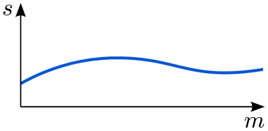
(a)

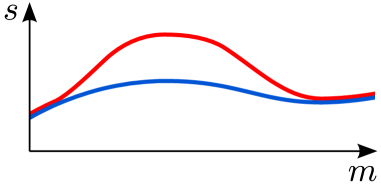
(b)

.

Figure 1: Abstract examples of sensorimotor interactions, see text for description.

To make this a bit clearer, consider the abstract example of a sensorimotor interaction between an agent and its environment that is depicted in Figure 1a, where the horizontal and vertical axes correspond to the agent’s motor and sensor spaces, respectively. When the agent maneuvers through its motor space (i.e. it translates its motor state left and right along the horizontal axis), it observes a stable sensory feedback pattern, which can be plotted as a curve. In this very simple example, the agent can easily learn a predictive model to capture the laws of its sensorimotor interaction. There is no reason for the agent to assume that the environment has a state, which is different from the agent’s own internal state. Indeed, the agent does not even have any reason to assume that there is any such thing as an environment. From the agent’s point of view, the whole world seems perfectly deterministic and completely controllable. Furthermore, there is no point for this agent to maintain a memory of any sort, such as an internal state (as opposed to its physical state, i.e. the one of its body). The agent could perfectly control its sensorimotor apparatus without having to know anything about the past.

Now consider the case of another agent, whose sensorimotor interaction with the environment is depicted in Figure 1b. It has identical motors and sensors as the agent from the first example, but its situation is substantially different: for some of the configurations in its motor space, it always observes a stable sensory feedback, just like the first agent, but for a subpart of its motor space it observes two different sensory feedbacks for identical motor configurations. This second agent faces the problem that was outlined above in the description of the PP account for cognition (see Section II-B): the sensory signals that it observes depend on factors that are external to the agent itself (changes happening in the agent’s environment), and thus are not controllable by the agent. Furthermore, the agent has no means to directly measure the external factors. Were it to make memoryless predictions of sensory observations (like the first agent), it would perform at chance level at most. Its only way to improve its capability to make accurate predictions is by maintaining an internal representation that somehow estimates the external causes of sensory observations.

Many formalisms have been introduced in the literature to address this problem. For example, one common way (among many others) to include an internal state in a predictive model is to use a recurrent neural network, which incorporates temporal information into its predictions. The point here however is not simply that this is a problem that needs to be addressed in some way. Instead, this work looks at the bigger picture: what is the nature of the representational system of the brain, and how could it be implemented in an artificial agent? Without a clear connection to a comprehensive theory of brain organization, it is difficult to see how a computational model might be extended to a complete cognitive system.

PP and the SMCT offer such a theory of brain organization, to a sufficient extent. Following the above interpretation of the theories, we can postulate that the internal representation of external causes of sensorimotor observations is in the form of internal states, which encode hypotheses about how the flow of sensorimotor signals will unfold. Concretely, we can imagine the agent to store two internal models, each of which estimates one of the two curves that are plotted in Figure 1b. By assigning an activation level to each one of these internal models, the agent becomes equipped with a simple form of memory and the ability to test its hypotheses about external causes: the agent can make predictions about how its sensory input will change in response to changing its motor state. Sensory observations will lie on either one of the two curves, which will lead to the corresponding internal model to be selected. In this view, the agent, after learning, would not simply make different sensory observations, but it would perceive two distinct sensorimotor contexts, or contingencies.

It was already demonstrated in the literature that such a selection mechanism can be implemented (e.g. [10]). This paper addresses the problem of how an agent can autonomously discover the external state for the training of appropriate internal models. For the purpose of demonstrating how this can be achieved, the next section will introduce a mathematical formalization of the problem description.

IV Mathematical Formalization

We can formally describe the sensorimotor experience of an agent in the following way: as it explores its sensorimotor space, for example by following an exploratory control policy (such as [24]), the agent observes sequences of sensorimotor states $\mathbf{x}_{i}$. Here, $\mathcal{X}=\{\mathbf{x}_{i}\}$ is the set of possible sensorimotor states and corresponds to extero- as well as interoceptive signals, which also includes efferent copies of motor signals. In the examples described above, this set of sensorimotor states is that of all possible pairs $(m_{i},s_{i})=\mathbf{x}_{i}$ in the two-dimensional plane that is depicted in Figure 1.

We can describe the experience of the agent, as it follows an exploration policy $\pi$, as a stochastic process:

$$X^{\pi}=\left\{X_{t}=\mathbf{x}_{i}~{}:~{}t=1,\dots,n\right\}.$$ (1)

If we further assume that the set $\mathcal{X}$ of sensorimotor states is countable (it will later be shown how to relax this assumption to deal with continuous sensorimotor spaces), we can model the agent’s sensorimotor exploration as a discrete-time Markov chain $X_{1},X_{2},\dots,X_{n}$.

In this formulation, the task of the agent to minimize its error in predicting future states amounts to estimating the probability

$$\Pr(X_{t+1}=\mathbf{x}_{j}~{}|~{}X_{t}=\mathbf{x}_{i},\pi,E_{t}=\mathbf{e}_{k}),$$ (2)

which describes the probability of observing a transition from one sensorimotor state, $\mathbf{x}_{i}$, to another, $\mathbf{x}_{j}$, when generating motor commands according to the policy $\pi$. Additionally, we let the probability distribution depend on a latent variable $\mathbf{e}_{k}$, which represents the current “agent-environment configuration”: it summarizes all external factors that influence the outcome of the agent’s actions. For example, imagine a robot with a control policy to grasp a bottle: executing this policy will obviously only have a chance of success if there is a bottle in reach of the robot in the current situation. As another example, imagine two identical robots, standing in a corridor in front of two identical looking doors, one leading to a kitchen, the other leading to a dining room. The sequence of observations that the two robots would make when opening and passing through the respective doors would of course be very different (one would probably see a fridge, while the other would probably see a dining table). This environmental influence, or sensorimotor context, is summarized in an abstract way by the variable $\mathbf{e}_{k}$. In the above example (Figure 1b), $\mathbf{e}_{k}$ could be said to assume one of two values, corresponding to one of the plotted curves, respectively.

One might be inclined to think of the variable $\mathbf{e}_{k}$ as the set of all possible states of the entire universe. But this would of course be entirely misleading: instead, it is helpful to conceive of it as the most compact way to encode all qualitatively different situations the agent can face, given its sensorimotor apparatus. From this perspective, we can argue that a sensorimotor contingency corresponds to a property of the agent’s interaction with the world, when the value of the latent variable $\mathbf{e}_{k}$ is fixed. Taking again the example of object perception, we could say that a given $\mathbf{e}_{k}$ corresponds to an agent-environment configuration where a certain object is in front of the agent (as compared to the object for example being in a certain absolute position in “world coordinates”).

Thus, since $\mathbf{e}_{k}$ is a latent variable, the agent cannot easily estimate the above probability. What it does observe as it explores its sensorimotor space for a longer period of time (i.e. for large $n$) is the marginal probability distribution

$$Pr(X_{t+1}=\mathbf{x}_{j}~{}|~{}X_{t}=\mathbf{x}_{i},\pi)\\ =\sum_{\mathbf{e}_{k}}Pr(X_{t+1}=\mathbf{x}_{j}~{}|~{}X_{t}=\mathbf{x}_{i},\pi,E_{t}=\mathbf{e}_{k}).$$ (3)

The agent therefore has to demarginalize this observed state transition distribution by estimating the latent environmental causes of sensorimotor states.

One way that the agent can estimate the current state $\mathbf{e}_{k}$, once it has achieved a suitable demarginalization, is by tracking the likelihood of the individual models (corresponding to the individual terms of the sum in Equation 3) over time, that is, using the models to make predictions and comparing each prediction with actually observed future states and updating model likelihoods correspondingly. Importantly, this implies that the distinguishing property on which the agent relies to decide whether two sensorimotor states are similar or not is temporal adjacency: given a high likelihood of an internal model, corresponding to a hypothesis about a contingency, the agent assumes that the next observation will also originate from the same contingency, unless the agent itself disengages from it. Furthermore, the agent can test whether two sensorimotor states are part of the same contingency by trying to reach the one state from the other, by means of its own actions. If the agent can reliably transition between two states whenever a certain internal model has a high likelihood, it can safely assume that both states are part of the corresponding contingency and can update the model accordingly. On the contrary, if the agent cannot reach some sensorimotor state, it can be inferred that this state does not belong to the current contingency.

In the following, we will describe how we can utilize this property to formulate an algorithm to demarginalize the transition probability distribution and to discover latent structure, for an agent to learn predictive models of sensorimotor contingencies.

IV-A Contingencies as Clusters of Mutually Reachable States

Equation 3 describes the marginal probability distribution of state transitions, which an agent observes when following a policy $\pi$ for an extended amount of time. In the discrete case, this distribution can be captured in a transition probability matrix $T_{\pi}$ with entries

$$\left(T_{\pi}\right)_{i,j}=\Pr(X_{t+1}=\mathbf{x}_{j}~{}|~{}X_{t}=\mathbf{x}_{i},\pi),$$ (4)

where $\mathbf{x}_{i},\mathbf{x}_{j}\in\mathcal{X}$.

As argued above, sensorimotor states that belong to the same contingency share the property that the agent can transition between the states using its own actions, or in other words, they are “reachable” from one another for the agent. In contrast, states that are not reachable in this sense do not belong to the same sensorimotor contingency.

The task to discover contingencies within the flux of sensorimotor states can thus be reformulated as one of finding sets of sensorimotor states, for which the agent observes a high probability of transitioning within the set while following its policy, but observing transitions out of the set only with a low probability. Note that it is not generally possible to construct such sets by grouping together sensorimotor states based on how “similar” they are in sensorimotor space (measured for example by their Cartesian distance). While a state $\mathbf{x}_{i}\in\mathcal{X}_{p}$ might have a low distance to another state $\mathbf{x}_{j}\in\mathcal{X}\setminus\mathcal{X}_{p}$, they can be dissimilar from a reachability point of view: they do not co-occur in the same contingency (meaning for example that the agent cannot reach $\mathbf{x}_{j}$ from $\mathbf{x}_{i}$ using its own actions). We will see examples for such cases later in the descriptions of the simulation experiments. A consequence of this property is that standard clustering methods, such as K-means, will not find a valuable solution.

When interpreting the transition probability matrix $T_{\pi}$ as an adjacency matrix for a weighted graph, where nodes represent sensorimotor states and edges represent transition probabilities, then the task of discovering sensorimotor contingencies consequently translates into one of finding densely connected subgraphs within this graph, or said otherwise, finding a partition that separates graph clusters. A suitable partition $\mathcal{P}=\{\mathcal{X}_{1},\mathcal{X}_{2},\dots,\mathcal{X}_{k}\}$ of $\mathcal{X}$ (the nodes of the graph) into $k$ subsets, which satisfies the property of having high intra-subset transition probabilities and low transition probabilities in between subsets can be found with the following minimization:

$$\underset{\mathcal{P}}{\arg\min}\sum_{\mathcal{X}_{p}\in\mathcal{P}}\sum_{\begin{subarray}{c}\mathbf{x}_{i}\in\mathcal{X}_{p}\\ \mathbf{x}_{j}\in\mathcal{X}\setminus\mathcal{X}_{p}\end{subarray}}\Pr(X_{t+1}=\mathbf{x}_{j}~{}|~{}X_{t}=\mathbf{x}_{i},\pi)$$ (5)

$$=\underset{\mathcal{P}}{\arg\min}\sum_{\mathcal{X}_{p}\in\mathcal{P}}\sum_{\begin{subarray}{c}\mathbf{x}_{i}\in\mathcal{X}_{p}\\ \mathbf{x}_{j}\in\mathcal{X}\setminus\mathcal{X}_{p}\end{subarray}}\left(T_{\pi}\right)_{i,j}.$$ (6)

Such a partition should constitute a solution to the problem of the agent of discovering sets of states that correspond to different latent causes. Thus, given a suitable partition $\mathcal{P}$, the probability distribution in Equation 2 can be estimated as

$$\Pr(X_{t+1}=\mathbf{x}_{j}~{}|~{}X_{t}=\mathbf{x}_{i},\pi,E_{t}=\mathbf{e}_{k})\\ \sim\Pr(X_{t+1}=\mathbf{x}_{j}~{}|~{}X_{t}=\mathbf{x}_{i},\pi,\mathbf{x}_{i}\in\mathcal{X}_{k}),$$ (7)

V Computational Model

The minimization problem defined in Equation 6 is an instance of the mincut problem of cutting the transition probability graph (which has the transition probability matrix $T_{\pi}$ as its adjacency matrix) in such a way into $k$ components that the cut-crossing edges have minimal weight. Each of the components would correspond to sets of sensorimotor states with high “inter-reachability”, whereas transitions in between sets occur less frequently, thus matching the property of contingencies when viewed from a graph point of view as described above.

The idea to use graph clustering methods to partition a state graph has already been suggested in the reinforcement learning literature [25, 26], but with a different motivation: the aim of these works is to discover “subgoals”, to speed up learning convergence in reinforcement learning (see also [27]). The idea is that “bottlenecks” (such as doorways in a navigation task) are important subgoals when discovering a policy, and they can be characterized as state transitions with low probability between two clusters of densely connected states. Such transitions can be discovered by formulating a similar minimization problem as the one proposed above. In contrast, here we are interested in discovering densely connected clusters, which we interpret as sensorimotor contingencies.

We thus want to solve the mincut problem for the transition probability graph defined by the matrix $T_{\pi}$ to find a partition into $k$ components. This can be approximately achieved through spectral clustering [28], using the method suggested by Ng and colleagues [29], in the following way.

We first solve the eigenvalue problem for the transition probability matrix to find the $k$ largest eigenvalues $\lambda_{1},\lambda_{2},\dots,\lambda_{k}$ and associated eigenvectors $u_{1},u_{2},\dots,u_{k}$, and form the matrix

$$U=[u_{1}~{}u_{2}~{}\dots~{}u_{k}]\in\mathbb{R}^{m\times k}$$ (8)

where $m=|\mathcal{X}|$ is the number of discrete sensorimotor states that the agent can observe. The matrix $U$ is then normalized such that each row has unit length, resulting in the matrix $V$ with entries

$$V_{i,j}=\frac{U_{i,j}}{\sqrt{\sum_{l}U_{i,l}^{2}}}.$$ (9)

Treating each row in $V$ as a point in $\mathbb{R}^{k}$, we cluster them into $k$ clusters using K-means. Since each row in $V$ also corresponds to a row in the original transition probability matrix $T_{\pi}$, and thus to a state $\mathbf{x}\in\mathcal{X}$, the result of the spectral clustering provides us with the final partition of $\mathcal{X}$ into the $k$ subsets $\{\mathcal{X}_{1},\mathcal{X}_{2},\dots,\mathcal{X}_{k}\}$. The agent can then use this partition of states to train multiple internal models, one for each subset $\mathcal{X}_{i}$ (see Equation 7).

VI Simulation Experiments

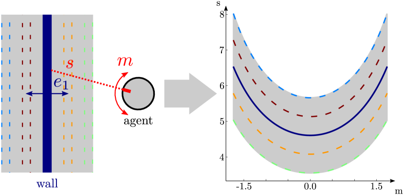
(a) simulated world: wall translates

(c) sensorimotor space

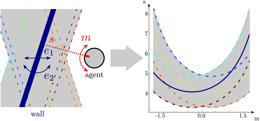
(b) simulated world: wall translates and rotates

(d) sensorimotor space

Figure 2: The simulation scenario that was used in the experiments. LABEL:sub@subfig:robotscenario_world_1d In the first variant, a wall is placed in front of the robot and moves towards and away from it. Several possible wall positions are indicated in different colors. LABEL:sub@subfig:robotscenario_world_2d In the second variant, the wall also rotates. In LABEL:sub@subfig:robotscenario_sms_1d–LABEL:sub@subfig:robotscenario_sms_2d the sensorimotor space is shown for the two variants, with observed manifolds plotted in color, corresponding to the shown wall configuration examples.

. .

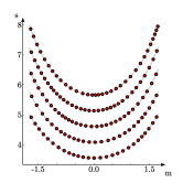
(a) Wall translating, five discrete positions.

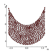
(b) Wall translating, continuous set of positions.

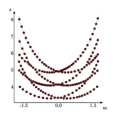
(c) Wall translating and rotating, six discrete positions.

Figure 3: The outcome of the agent’s initial exploration of the sensorimotor space, in three variants of the simulation experiment. Sensorimotor observations are plotted as gray dots, cluster centroids are shown as red circles.

To evaluate the method proposed above, a simplistic simulation scenario was designed with the purpose of highlighting several important aspects of the learning problem that a naive agent is facing when learning to interact with its environment. Consider the situation of an agent (a virtual robot) with a turnable base and a single laser range sensor, measuring the distance to the nearest obstacle in a straight line of sight (see Figures 2LABEL:sub@subfig:robotscenario_world_1d–LABEL:sub@subfig:robotscenario_world_2d). In front of the agent, in the otherwise empty environment, a movable wall is placed. As the agent explores its situation by generating motor commands, i.e. rotating around its base, it makes a sequence of observations. As long as the wall remains static, these observations all lie on a one-dimensional manifold in the agent’s two-dimensional sensorimotor space. However, in this scenario, the wall is randomly moved into new positions. As the wall changes positions, also the manifold in sensorimotor space changes, on which the observations lie that the agent makes. This can be seen in Figures 2LABEL:sub@subfig:robotscenario_sms_1d–LABEL:sub@subfig:robotscenario_sms_2d, which show the agent’s two-dimensional sensorimotor space (with the motor degree of freedom along the horizontal axis, and the sensory input along the vertical axis): for each distinct state of the world (i.e. position and orientation of the wall), the agent’s observations lie on a different curve.

In this simulation scenario, the latent environmental state $\mathbf{e}_{k}$ (cf. Equation 2) consists of the degrees of freedom of the wall: its position and orientation. For each distinct state, the agent’s exploration results in observations lying on a corresponding distinct manifold. When considering this process in terms of the marginal probability distribution described by Equation 3, each individual state of the environments corresponds to one of the summands, and thus a distinct distribution.

The agent however only has access to its own sensor and motor states, whereas the state of the wall is unknown to it. It also has no information about when the environment changes states. But the sensory feedback that it receives when exploring its environment is directly influenced by the state of the environment. From an external perspective, the observations made by the agent can be characterized as sequences of curve segments, a new segment beginning each time when the environment changes states. However, the agent a priori does not know about the existence of this structure in the data. It experiences observations distributed in sensorimotor space, without knowing that they belong to distinct subspaces, or manifolds. From the agent’s point of view, the samples are generated from the marginal probability distribution of sensorimotor state transitions, see Equation 3. When trying to directly estimate a model of the sample distribution from all the samples taken together, the agent would thus face the difficulty of having a large sensory variance associated with each transition, which in turn would result in a low accuracy for prediction.

However, as suggested above, the agent can solve this problem by clustering observations together in terms of how well it can reach them from one another, as opposed to how similar they appear (as for example measured by their Cartesian distance in sensorimotor space), thereby demarginalizing the probability distribution, allowing the agent to estimate multiple separate internal models, to account for different latent states.

In a first step, the continuous sensorimotor space of the agent is discretized in an initial sensorimotor exploration phase, to construct the set of sensorimotor states $\mathcal{X}$: The agent generates observations by exploring its motor space and observing sensory responses, across a timespan long enough for the environment to visit all of its states. In the experiments, a Gaussian random walk was used as exploration policy $\pi$ for the agent’s motor outputs while the environment’s state changed at each time step with a probability of $0.1$ (also performing a Gaussian random walk in its own state space $\mathcal{E}=\left\{\mathbf{e}_{i}\right\}$), thus allowing the agent to explore each constant state of the environment on average for 10 time steps. K-means is then applied on the set of observations to obtain a discretization of the sensorimotor space into $r$ states, resulting in the set of sensorimotor states $\mathcal{X}=\{\mathbf{x}_{i}\}$, $i=1,\dots,r$, $\mathbf{x}_{i}=(m_{i},s_{i})^{T}$. The outcome is plotted in Figures 3LABEL:sub@subfig:kmeans_5x1–LABEL:sub@subfig:kmeans_3x2 for different versions of the scenario. Subsequently, sensorimotor observations are classified as one of these states using nearest-neighbor classification.

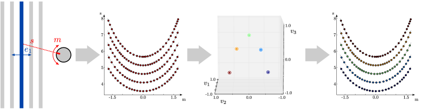
MMMMMMMM

(a) simulated world

MMMMMMMMM

(b) sensorimotor space

MMMMMMM

(c) spectral space

MMMMMMMMMM

(d) sensorimotor contexts

Figure 4: Overview of Simulation 1. LABEL:sub@subfig:simulation_1a The wall moves into five distinct positions, shown in gray. The five distinct configurations can also clearly be seen in the agent’s sensorimotor space LABEL:sub@subfig:simulation_1b, as well as in its spectral projection LABEL:sub@subfig:simulation_1c. In the latter, the outcome of the spectral clustering is indicated by the different colors, showing that LABEL:sub@subfig:simulation_1d the five sensorimotor contexts have correctly been discovered.

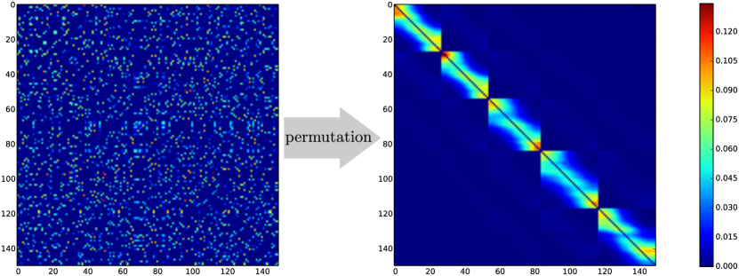
Figure 5: Via a permutation of the transition probability matrix $T_{\pi}$, some of the underlying structure of the sensorimotor interaction of the agent with its environment becomes apparent.

The agent then continues to explore its sensorimotor space for a fixed amount of time and thus observes a sequence of sensorimotor states. Above it was argued that sensorimotor contingencies are characterized by sets of states that are “inter-reachable” for the agent, meaning that it can transform any state within the set into any other state from the same set, with its own actions. The agent thus only requires to retain information about state transitions: knowledge about which state transitions are possible is sufficient to derive which states can be reached from one another. We therefore remove from the sequence of observed sensorimotor states all duplicate entries, such that we obtain a sequence of states (cf. Equation 1) in which each pair of subsequent elements correspond to an observed state transition:

$$X^{\pi}=\left\{X_{t}=\mathbf{x}_{i}~{}:~{}t=1,\dots,n\right\},~{}\textrm{s.t.}~{}\forall~{}t:~{}X_{t}\neq X_{t+1}.$$ (10)

Based on these observed state transitions, the transition probability matrix $T_{\pi}$ is then constructed (cf. Equation 4), where each row is normalized to sum up to $1$ to form a probability mass function. Spectral clustering is then applied as per the method presented in Section V to obtain a partition of the set of sensorimotor states.

In the following, several simulation runs will be presented, to visualize the result of the learning method, and to point out properties of the learning problem that a naive agent is facing when trying to learn sensorimotor contingencies as described above.

VI-A Simulation 1: Spectral Transform of Sensorimotor States

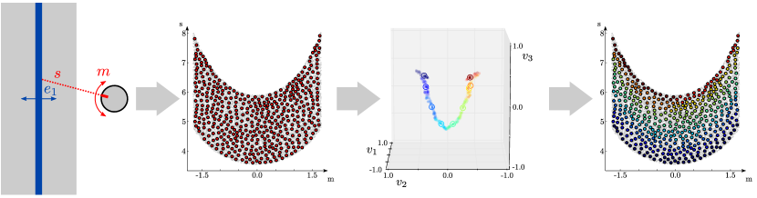
MMMMMMMM

(a) simulated world

MMMMMMMMM

(b) sensorimotor space

MMMMMMM

(c) spectral space

MMMMMMMMMM

(d) sensorimotor contexts

Figure 6: Overview of Simulation 2. LABEL:sub@subfig:simulation_2a In this variant, the wall moves freely within an interval of possible positions (shown as a gray area). LABEL:sub@subfig:simulation_2b Distinct manifolds are no longer visible in sensorimotor space, but LABEL:sub@subfig:simulation_2c its projection into spectral space results in a distribution of the sensorimotor states along a one-dimensional manifold, capturing the one degree-of-freedom of the environment. LABEL:sub@subfig:simulation_2d The spectral clustering successfully captures the structure of the interaction: discovered sensorimotor contexts match the curvature of the continuum of manifolds.

Consider first the case of the simulation scenario where the wall only moves towards and away from the agent into five distinct states, while its orientation is held constant (see Figure 4 for an overview of the simulation experiment). Figure 5 shows the transition probability matrix $T_{\pi}$ that was constructed in this case. We can uncover some of the structure of the interaction by permuting the rows and columns: Since the generation of sensorimotor states through K-means does not carry any information about the topology of the sensorimotor space, the ordering of rows and columns is initially random. However, for the purpose of visualization, we can permute them to match the true topology of the data. This way it becomes easily visible that each of the states of the wall manifests itself for the agent as a “cluster” of states between which the agent can transition with high probability, whereas transitions between the clusters have a low probability. This can be seen in the figure as blocks of entries with high values along the diagonal of the matrix, one for each of the states of the environment. Note that the fact that some of the sensorimotor states have a higher probability to be transitioned to, in particular ones lying close to the left and right limits of the motor space, is due to the way that cluster centroids were placed in sensorimotor space by the K-means algorithm: because of the curvature of the manifolds, the centroids are more “packed” towards the center of the motor space and more spread apart towards the ends, rendering it overall more likely for the agent to observe the centroids lying close to the ends of the motor space.

When interpreting $T_{\pi}$ as an adjacency matrix for a graph, as suggested above in Section IV-A, each of these blocks corresponds to a densely connected subgraph within this graph. Note that the reordering has no effect whatsoever on the result of the learning method, and is therefore unnecessary. It was only done here once for the purpose of visualization, and normally is not part of the learning method.

In the spectral clustering step, the matrix $V\in\mathbb{R}^{m\times k}$ is constructed based on an eigenvalue decomposition of the matrix $T_{\pi}$, as described in Section V. Each of the $k$ rows in $V$ corresponds to exactly one sensorimotor state $\mathbf{x}_{i}$, and is treated as a coordinate in an $m$-dimensional “spectral space”. The $m$ dimensions of the spectral space in turn correspond to the eigenvectors associated to the $m$ strongest eigenvalues of $T_{\pi}$. To visualize this mapping of sensorimotor space into the spectral space, Figure 4c shows a plot of a projection of the $k$ points into the three-dimensional subspace of the three strongest eigenvalues: it can be seen that all points lie in one of five dense clusters. The actual clustering is performed using K-means in the $m$-dimensional spectral space, where $m$ is also the number of clusters to be found.

Selecting the correct number of clusters $m$ of course plays an important role in the outcome, as in any clustering method. However, for the purpose of this discussion, the problem of how to estimate $m$ is not the focus and instead a good value is manually selected. However it should be noted that methods exist to automatically estimate the number of clusters [30]. In this version of the scenario, it is set to $m=5$, to match the number of discrete positions that the wall is entering. Figure 4d shows the result of the clustering of the sensorimotor states: it can be seen that indeed each of the five dense clusters in spectral space groups together all sensorimotor states that belong to one of the position of the wall.

VI-B Simulation 2: The Topology of the Internal State Representation

We can learn more about the topology of the distribution of sensorimotor states in spectral space when considering another variant of the scenario: in this variant, the wall changes positions in form of a continuous Gaussian random walk. The latent variable $\mathbf{e}$ therefore assumes values from an interval, instead of only five discrete values as before. Figure 6 shows an overview of this version of the simulation experiment. Here it can be seen, that the states are no longer clearly separated in spectral space, but instead have a curve-like distribution. Furthermore, as indicated by the color code, this curve-like distribution can be seen as capturing the one degree-of-freedom of the environment: Sensorimotor states that lie at the bottom of sensorimotor space (i.e. states that are observed when the wall is in the position that is closest to the agent) have been mapped to the left end of the curve. As we move rightwards along the curve, the positions of states move upwards in sensorimotor space, until finally, at the other end of the curve, all states are gathered that correspond to the topmost manifold in sensorimotor space (i.e. states that are observed when the wall is in the position that is farthest away from the agent). Note that what is shown in the figure is a three-dimensional projection of a higher-dimensional distribution, in this case $m=10$. Because of the normalization that is done in Equation 9, the points actually lie on the surface of an $m$-dimensional hypersphere.

The result of applying spectral clustering in this case is shown in Figure 6d. It can be seen that overall, sensorimotor states that are located close to similar manifolds (i.e. wall positions) have been clustered together. Note however, that the top-most clusters are “broken apart” in the center: this is a result of choosing a larger value for the parameter $m$ in the K-means step. These clusters that represent curve segments could be merged together in a subsequent step, to improve the quality of the result. How and why the agent could do this will be discussed in the conclusion of this article.

To understand why the sensorimotor points are distributed in a curve-like way in spectral space, that is, along a one-dimensional manifold on the surface of the $m$-dimensional hypersphere, it is again helpful to think of the matrix $T_{\pi}$ as an adjacency matrix of a graph. The construction of the spectral space can then be seen as a means to map out the graph in $m$-dimensional space, such that nodes (i.e. sensorimotor states) that are connected via edges with high weights are placed close together. Transitions between sensorimotor states with higher probability can thus be seen as “springs” that pull these states together in spectral space. In the case of the first simulation, the result is quite clear: only transitions within one of the five clusters had relatively high probabilities, and thus the states of each of the clusters were “pulled together”, effectively collapsing them into five almost point-like distributions. In the case of the second simulation however, the situation is a bit different: Each sensorimotor state can now be observed not only in a single, but many wall positions. Importantly, this means that for a given sensorimotor state, the agent will observe transitions to different other states, depending on the exact position of the wall (for example when moving left in motor space, for one wall position it might transition “left and down” to another state, whereas it might transition ”left and up” when the wall is slightly farther away). As a result, similar sets of sensorimotor states are observed by the agent when the wall is in similar configurations, and thus, they are arranged closely together in spectral space. On the other hand, sensorimotor states that only occur in very different wall configurations are not bound together by high transition probabilities, and thus are mapped further apart in spectral space. This behavior results in the generation of the point distribution that can be seen in Figure 6c.

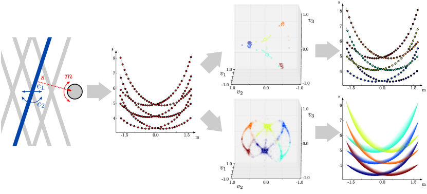
MMMMMMMM

(a) simulated world

MMMMMMMMM

(b) sensorimotor space

MMMMMMM

(c) spectral space

MMMMMMMMMM

(d) sensorimotor contexts

Figure 7: Overview of Simulation 3. LABEL:sub@subfig:simulation_3a In this variant, the wall not only translates but also rotates, resulting in intersecting manifolds in sensorimotor space LABEL:sub@subfig:simulation_3b. The upper and lower paths of LABEL:sub@subfig:simulation_3c–LABEL:sub@subfig:simulation_3d show the result of the spectral clustering for the cases of clustering observations and transitions, respectively (see text for details).

As a first qualitative result, it can thus be said that through the presented learning method, a naive agent constructs an internal representational space (the spectral space), in which observations happen to be distributed along a one-dimensional manifold. This one-dimensional manifold happens to correspond nicely to the actual one-dimensional latent state space $\mathbf{e}$ of the environment, even though at no point was any information about the latent variable put into the learning system. Furthermore, the internal representational space of the agent stabilizes the agent’s perception of the world: instead of trying to directly build up a predictive model of its sensorimotor interaction, which is difficult because of large variances in sensory observations as discussed further above, the agent could first construct the internal space and subsequently select subsets of observations, based on which it could train individual predictive models. In a way this allows the agent to virtually “freeze” the environment, to improve its learning.

VI-C Simulation 3: Ambiguity in Sensorimotor States

So far, only simulations have been described in which the wall changed its position, but not its orientation. What this means is that when the wall moves, the manifold of observations in sensorimotor space translated parallel to the axis corresponding to the sensory input dimension (the vertical axis in the figures above). This in turn means that every point in the agents sensorimotor space unambiguously belonged to exactly one manifold. The agent thus could identify the latent state of the environment from a single observation, and would be able to predict what other sensorimotor states to expect: those lying on the same manifold.

In more technical terms, it can be said that the environment in the above examples was Markovian: to make an accurate prediction about the next sensorimotor state, the agent in principle only has to know the current sensorimotor state. The assumption about the state distribution being Markovian is often made in the reinforcement learning literature, but cannot be assumed to be true in general. In fact, often a state space is specifically designed in such a way that it is compact and casts the problem into a setting in which the Markovian assumption holds. But of course, this is not possible when the goal is to develop generic learning mechanisms, where the task knowledge of the human designer cannot be incorporated into the learning system.

To see what situation a naive agent is facing when confronted with an environment in which the Markovian assumption does not hold, consider the variant of the simulation scenario where the wall not only moves, but also rotates (see Figure 7 for an overview of this third simulation experiment). The key difference to the previous experiments, is that the manifolds in sensorimotor space are now crossing (see Figure 7b). At each intersection point, the agent can now no longer predict what other observations it will make, based solely on the current observation. The sensorimotor states at the intersection points are ambiguous, belonging to multiple distinct contexts. This of course has an important impact on the transition probabilities that the agent observes: while transitions along non-intersecting curve segments have locally Markovian distributions as in the previous simulations, transitions from intersection points can end in sensorimotor states lying on any of the intersecting manifolds.

When interpreting the mapping from sensorimotor space to spectral space again in terms of a graph with “spring-like” edges, it becomes clear why the above property of sensorimotor states lying on intersection points being connected to other states from multiple manifolds has a strong impact on the spectral mapping. This can be seen in the top plot of Figure 7c, which shows again a three-dimensional projection of the (in this case six-dimensional) spectral space. It can be seen that states belonging to different contexts are no longer clearly grouped together in spectral space, nor do they seem to be organized in a low-dimensional manifold. Instead, states from different contexts are “pulled together” by the ambiguous states, resulting in a distribution that – at least in the three-dimensional projection – appears to be “folded” in a non-trivial way. The outcome of the K-means clustering in spectral space, shown in the upper plot in Figure 7d, still correctly separates sensorimotor states into different contexts. However, two things have to be noted: Firstly, the clustering does not always produce the result that is shown here, but instead sometimes incorrectly combines curve segments from intersecting manifolds. This, as well, offers the interpretation that the distribution of sensorimotor states is rather complex, not only in the three-dimensional projection but also in the actual six-dimensional spectral space. Secondly, the hard clustering that is produced by K-means of course results in each sensorimotor state being associated to exactly one cluster, or context. However, the sensorimotor states that lie at the intersection point between manifolds should actually be considered as belonging to both of the intersecting manifolds.

A first step towards resolving these issues is to change the representation of the agent to the space of transitions between observations. By doing this, the method described above no longer clusters together observations, but frequently co-occurring transitions between observations. A similar strategy has also been successfully applied for example by Mnih et al. to disambiguate observations [16]. Minh et al. used sequences of video frames as input to their reinforcement learning system instead of single frames, which might be ambiguous.

The overall method remains unchanged, with the only adaptation being the notion of state: not points in sensorimotor space, but transitions between points are treated as states. To make the distinction explicit, a superscript arrow will be used in the notation of this new definition of state: $\mathcal{X}^{\rightarrow}=\{\mathbf{x}^{\rightarrow}_{d_{i,j}}\}$, where $d_{i,j}$ is an index, and the state $\mathbf{x}^{\rightarrow}_{d_{i,j}}=(\mathbf{x}_{i},\mathbf{x}_{j})$ corresponds to a transition from one K-means cluster, $\mathbf{x}_{i}$, to another, $\mathbf{x}_{j}$. Consequently, the state transition probability (cf. Equation 2) becomes

$$\Pr(X_{t+1}=\mathbf{x}^{\rightarrow}_{d_{j,k}}~{}|~{}X_{t}=\mathbf{x}^{\rightarrow}_{d_{i,j}},\pi,E_{t}=\mathbf{e}_{l}),$$ (11)

and entries in the transition probability matrix $T^{\rightarrow}_{\pi}$ become

$$\left(T^{\rightarrow}_{\pi}\right)_{d_{i,j},d_{j,k}}=\Pr(X_{t+1}=\mathbf{x}^{\rightarrow}_{d_{j,k}}~{}|~{}X_{t}=\mathbf{x}^{\rightarrow}_{d_{i,j}},\pi).$$ (12)

The lower parts of Figures 7LABEL:sub@subfig:simulation_3c–LABEL:sub@subfig:simulation_3d show the outcome of applying the algorithm when using this new definition of state. Each point in spectral space in this case represents one transition between clusters in sensorimotor space. Transitions within one manifold have again been nicely grouped together, forming six clearly visible clusters of states that can easily be separated using K-means.

VII Conclusion

Despite the impressive progress that has been made in machine learning research recently, we still do not know how to efficiently implement the learning of generic knowledge in artificial agents, such as robots. This article offered as a perspective on this topic to take inspiration from two recent developments in the cognitive science literature: predictive processing approaches to cognition, and the sensorimotor contingencies theory of perception. More specifically, this paper is in line with recent works that suggest a combination of PP and the SMCT [5, 7].

According to PP, the cognitive system of adaptive agents has to maintain a hierarchical model of the latent causes of sensory observations. To answer the question of how a naive agent could autonomously learn about these latent causes, this article borrowed the concept of sensorimotor contingency from the SMCT of perception: an agent should try to engage in predictable sensorimotor interactions with its environment, by the means of which it perceives sensorimotor contexts (or contingencies). This idea was formally cast into a computational model as an instance of the mincut problem on a graph of sensorimotor state transitions, and spectral clustering was proposed as a method to solve this problem.

In the proposed model, the agent discovers sensorimotor contexts as sets of sensorimotor states that, for the agent, are reachable from one another: if it observes one state and, after acting, observes another state with high probability, then the agent can assume that these two states belong to the same context. It was demonstrated in a series of simulation experiments that with the proposed method, a naive agent can successfully discover sensorimotor contexts.

In the presented implementation of the method, the agent’s knowledge about the discovered sensorimotor contexts was represented in a very simple way: the set of sensorimotor states was partitioned, resulting in a description of sensorimotor contexts in the form of subsets of this set, in conjunction with a transition probability matrix. As a next step, it would be possible to train more accurate predictive models for each of the discovered sensorimotor contexts, to improve the agent’s capability to predict the flow of sensorimotor observations. But already in this very simple implementation, the agent can be said to reduce its overall prediction error: Were it to make predictions about sensorimotor state transitions directly (i.e. without first discovering the different sensorimotor contexts), it would have to base its predictions on the estimate of the marginal probability distribution (Equation 3). In contrast, as discussed above, the agent can demarginalize the distribution via the discovery of sensorimotor contexts, effectively allowing it to estimate the latent variable $\mathbf{e}$ and to make its predictions under the posterior probability described by Equation 7. The posterior probability distribution necessarily has a lower entropy than the marginal probability distribution, which is equivalent to saying that the agent improves its overall ability to predict [3].

Two variants for defining the notion of “sensorimotor state” were used in the simulation experiments: either prototype points in sensorimotor space (placed using K-means), or transitions between such prototypes. As long as the space of sensorimotor observations is unambiguous, the former definition is suitable for the agent to recognize sensorimotor contexts. However, when sensorimotor observations can belong to more than just a single context, this becomes problematic, as was demonstrated in the simulation experiments. In that case, ambiguous observations were arbitrarily assigned to one context. By implication this means that the agent would always perceive these observations as belonging to a certain context, even when they occur within another. It was demonstrated that this problem could be solved by instead clustering transitions between prototypes. In that case, the agent would no longer recognize a sensorimotor context directly via the set of observations that occur within that context, but via transitions between observations. Said otherwise, the agent has to act in order to perceive a context. It should be noted however that it would still not be strictly necessary for the agent to act to perceive anything. Instead, when an observation unambiguously belongs to only one context (i.e. all transitions from and to this observation belong to the same context), then there is no reason to assume that the agent would first have to move to perceive the context or contingency.

In all of the presented simulation experiments, the number of contexts to be discovered was manually fixed by specifying the number of clusters that should be found by the spectral clustering algorithm. Of course this should be done in an autonomous way instead, which will be addressed in future work. One possibility would be to use a method to estimate a suitable number of clusters [30], as suggested above. However, it may be more natural to approach this difficulty in the scope of the related question of how a system should construct a representational hierarchy, in the following way. Initially, a large number of clusters could be formed, resulting in a too finely grained partition of sensorimotor states. But in a subsequent step, the next level of the representational hierarchy could be constructed by reapplying the same algorithm, but treating clusters as “meta-states”: While the agent would continue to interact with its environment, it would recognize observations as belonging to a number of the initially discovered contexts, or meta-states, namely those that together constitute the actual manifold in sensorimotor space, on which the observations are distributed. It would therefore observe transitions between these contexts to occur with a high probability, comparable to the high probability of transitions between sensorimotor states that belong to the same manifold. The same process of discovering densely connected subgraphs (by constructing a transition probability matrix and applying the spectral clustering algorithm) could thus be repeated at this stage. The outcome would be sets of clusters from the initially too finely grained partition of sensorimotor states. As such, it seems like it might not be necessary to introduce a further mechanism for estimating a suitable number of clusters at each hierarchical level – the method, when repeated across levels of a hierarchy, could be seen as a hierarchical clustering method that iteratively combines more and more clusters.

Another direction of future work is to explore how the presented method can be utilized in the context of reinforcement learning. What the agent discovers is a compact representation of latent states of the environment, which might be used as feature representation. Indeed, it has been shown by Mahadevan and Maggioni that a spectral transformation similar to the one used in this paper can be used for the construction of a basis, to estimate a value function [31].

Finally, the role of the exploration policy in the discovery of sensorimotor contexts, or contingencies, should be investigated. In this work, the agent relied on a simple random walk as exploration policy, which, while sufficient, certainly is a sub-optimal way to gather information about the sensorimotor interaction and the environment. A more directed search strategy could certainly speed up the learning process significantly.

Nikolas J. Hemion Dr. Nikolas Hemion received his Ph.D. degree in Intelligent Systems in 2013 from the Research Institute for Cognition and Robotics, Bielefeld University, Germany. During his doctoral studies, he collaborated with the Honda Research Institute Europe, and visited the Centre for Robotics and Neural Systems, Plymouth University, UK. Subsequently he joined the AI Lab at Aldebaran as senior researcher, and was appointed as director of the AI Lab in 2015. Nikolas is also co-director of the H2020 innovative training network APRIL. His research interests lie in cognitive architecture and model learning for cognitive robotics, and self-organized learning of sensorimotor representations.

References

- [1] R. S. Sutton and A. G. Barto, Reinforcement learning: An introduction. MIT press, 1998.
- [2] D. M. Wolpert, R. C. Miall, and M. Kawato, “Internal models in the cerebellum,” Trends in cognitive sciences, vol. 2, no. 9, pp. 338–347, 1998.
- [3] K. J. Friston and K. E. Stephan, “Free-energy and the brain,” Synthese, vol. 159, no. 3, pp. 417–458, 2007.
- [4] A. Clark, “Whatever next? predictive brains, situated agents, and the future of cognitive science,” Behavioral and Brain Sciences, vol. 36, no. 03, pp. 181–204, 2013.
- [5] A. K. Seth, “A predictive processing theory of sensorimotor contingencies: explaining the puzzle of perceptual presence and its absence in synesthesia,” Cognitive neuroscience, vol. 5, no. 2, pp. 97–118, 2014.
- [6] K. Friston, “The free-energy principle: a unified brain theory?” Nature Reviews Neuroscience, vol. 11, no. 2, pp. 127–138, 2010.
- [7] A. Laflaquiere, N. J. Hemion, M. G. Ortiz, and J.-C. Baillie, “Grounding perception: a developmental approach to sensorimotor contingencies,” in IROS Workshop on Sensorimotor Contingencies for Robotics. IEEE, 2015.
- [8] A. K. Seth, “The cybernetic bayesian brain: From interoceptive inference to sensorimotor contingencies,” 2015.
- [9] J. K. O’Regan and A. Noë, “A sensorimotor account of vision and visual consciousness,” Behavioral and brain sciences, vol. 24, no. 05, pp. 939–973, 2001.
- [10] M. Haruno, D. M. Wolpert, and M. Kawato, “Mosaic model for sensorimotor learning and control,” Neural computation, vol. 13, no. 10, pp. 2201–2220, 2001.
- [11] J. Kober, J. A. Bagnell, and J. Peters, “Reinforcement learning in robotics: A survey,” The International Journal of Robotics Research, p. 0278364913495721, 2013.
- [12] F. Stulp and O. Sigaud, “Robot skill learning: From reinforcement learning to evolution strategies,” Paladyn, Journal of Behavioral Robotics, vol. 4, no. 1, pp. 49–61, 2013.
- [13] A. J. Ijspeert, J. Nakanishi, and S. Schaal, “Movement imitation with nonlinear dynamical systems in humanoid robots,” in Robotics and Automation, 2002. Proceedings. ICRA’02. IEEE International Conference on, vol. 2. IEEE, 2002, pp. 1398–1403.
- [14] Y. Bengio, “Learning deep architectures for ai,” Foundations and trends® in Machine Learning, vol. 2, no. 1, pp. 1–127, 2009.
- [15] S. Levine, C. Finn, T. Darrell, and P. Abbeel, “End-to-end training of deep visuomotor policies,” arXiv preprint arXiv:1504.00702, 2015.
- [16] V. Mnih, K. Kavukcuoglu, D. Silver, A. Graves, I. Antonoglou, D. Wierstra, and M. Riedmiller, “Playing atari with deep reinforcement learning,” arXiv preprint arXiv:1312.5602, 2013.
- [17] M. E. Taylor and P. Stone, “Transfer learning for reinforcement learning domains: A survey,” The Journal of Machine Learning Research, vol. 10, pp. 1633–1685, 2009.
- [18] K. Ferguson and S. Mahadevan, “Proto-transfer learning in markov decision processes using spectral methods,” Computer Science Department Faculty Publication Series, p. 151, 2006.
- [19] M. E. Taylor, N. K. Jong, and P. Stone, “Transferring instances for model-based reinforcement learning,” in Machine learning and knowledge discovery in databases. Springer, 2008, pp. 488–505.
- [20] A. Laflaquiere, A. V. Terekhov, B. Gas, and J. K. O’Regan, “Learning an internal representation of the end-effector configuration space,” in Intelligent Robots and Systems (IROS), 2013 IEEE/RSJ International Conference on. IEEE, 2013, pp. 1230–1235.
- [21] K. Friston, R. Adams, L. Perrinet, and M. Breakspear, “Perceptions as hypotheses: Saccades as experiments,” Frontiers in psychology, vol. 3, p. 151, 2012.
- [22] D. L. Philipona and J. K. O’regan, “Color naming, unique hues, and hue cancellation predicted from singularities in reflection properties,” Visual neuroscience, vol. 23, no. 3-4, pp. 331–339, 2006.
- [23] A. Laflaquière, J. K. O’Regan, S. Argentieri, B. Gas, and A. V. Terekhov, “Learning agent’s spatial configuration from sensorimotor invariants,” Robotics and Autonomous Systems, vol. 71, pp. 49–59, 2015.
- [24] P.-Y. Oudeyer, F. Kaplan, and V. V. Hafner, “Intrinsic motivation systems for autonomous mental development,” Evolutionary Computation, IEEE Transactions on, vol. 11, no. 2, pp. 265–286, 2007.
- [25] Ö. Şimşek, A. P. Wolfe, and A. G. Barto, “Identifying useful subgoals in reinforcement learning by local graph partitioning,” in Proceedings of the 22nd international conference on Machine learning. ACM, 2005, pp. 816–823.
- [26] S. Mannor, I. Menache, A. Hoze, and U. Klein, “Dynamic abstraction in reinforcement learning via clustering,” in Proceedings of the twenty-first international conference on Machine learning. ACM, 2004, p. 71.
- [27] A. G. Barto and S. Mahadevan, “Recent advances in hierarchical reinforcement learning,” Discrete Event Dynamic Systems, vol. 13, no. 4, pp. 341–379, 2003.
- [28] U. Von Luxburg, “A tutorial on spectral clustering,” Statistics and computing, vol. 17, no. 4, pp. 395–416, 2007.
- [29] A. Y. Ng, M. I. Jordan, Y. Weiss et al., “On spectral clustering: Analysis and an algorithm,” Advances in neural information processing systems, vol. 2, pp. 849–856, 2002.
- [30] A. K. Jain, “Data clustering: 50 years beyond k-means,” Pattern recognition letters, vol. 31, no. 8, pp. 651–666, 2010.
- [31] S. Mahadevan and M. Maggioni, “Proto-value functions: A laplacian framework for learning representation and control in markov decision processes.” Journal of Machine Learning Research, vol. 8, no. 2169-2231, p. 16, 2007.