Condensate flow in holographic models in the presence of dark matter

Abstract

Holographic model of a three-dimensional current carrying superconductor or superfluid with dark matter sector described by the additional $U(1)$-gauge field coupled to the ordinary Maxwell one, has been studied in the probe limit. We investigated analytically by the Sturm-Liouville variational method, the holographic s-wave and p-wave models in the background of the AdS soliton as well as five-dimensional AdS black hole spacetimes. The two models of p-wave superfluids were considered, the so called $SU(2)$ and the Maxwell-vector. Special attention has been paid to the dependence of the critical chemical potential and critical transition temperature on the velocity of the condensate and dark matter parameters. The current $J$ in holographic three-dimensional superconductor studied here, shows the linear dependence on $T_{c}-T$ for both s and p-wave symmetry. This is in a significant contrast with the previously obtained results for two-dimensional superconductors, which reveal the $(T-T_{c})^{3/2}$ temperature dependence. The coupling constant $\alpha$, as well as, chemical potential $\mu_{D}$ and the velocity $S_{D}$ of the dark matter, affect the critical chemical potential of the p-wave holographic $SU(2)$ system. On the other hand, $\alpha$, dark matter velocity $S_{D}$ and density $\rho_{D}$ determine the actual value of the transition temperature of the same superconductor/superfluid set up. However, the dark matter does not affect the value of the current.

1 Introduction

The application of gauge/gravity duality mal98 -sac12 to study experimentally relevant systems has resulted in number of important findings erdbook ; zaanen-book . Among the most intriguing issues is the universal ratio between the viscosity and entropy density in the strongly interacting system, which has helped to understand the viscosity of the quark-gluon plasma. Other equally important findings are related to strongly coupled condensed matter systems and their transport properties. They include analysis of holographic superconductors, superfluids and their behavior under special conditions. Based on the AdS/CFT correspondence the description of holographic s-wave superconductor was presented gub08 -mae08 and soon after the method was adopted to take into account p gub08 -liu15 and d-wave superconductors che10 -zen10 . In amo14 a generalization of the standard holographic p-wave superconductor with two interacting vector order parameters was investigated. The model was proposed as a holographic effective theory of a strongly coupled ferromagnetic superconductor.

The aforementioned studies were generalized in many ways, e.g., back-reaction of the order parameter on spacetime metric was considered enabling the second order phase transition to be replaced by the first order one amm10p , the gravitational background of AdS soliton hor98 was proposed to study holographic insulator/superconductor transition at zero temperature nis10 -akh11 . Further, the studies concerning Gauss-Bonnet gravity, non-linear electrodynamics and Weyl corrections on p-wave holographic phase transitions were elaborated pan11 -jin12 , On the other hand, holographic vortices and droplets influenced by magnetic field were discussed in alb08 -roy12 .

The early applications of the gravity methods to study holographic superconductors described by the scalar field in the appropriate gravity background have soon been extended to other symmetries and systems with super-current.

Properties of current carrying superconductors have recently been studied by means of AdS/CFT correspondence with the hope to unveil the novel strong coupling properties of superconductors with a constant velocity or super-current gub08a ; hor08 ; her09a ; bas09 ; son10 ; are10 ; zen11 ; zen13 ; wu14 ; amm10 ; ama13 ; ama14 ; lai16 ; bas09a . In the gauge/gravity duality the super-current is introduced by the spatial component of the gauge field depending on the radial direction. Close to the boundary of the spacetime the constant part is interpreted as superfluid velocity, while the component in front of the next leading term ($\propto 1/r^{2}$) is related to the current in the dual field theory. Continuation of the work hor08 , constitutes the paper her09a in which the authors consider superfluid with superfluid current flowing through the system. It was established that there was a first order phase transition between superfluid and the normal phase in the case when one changed the superfluid current. At high temperatures the phase transition became a second order. In bas09 , in the background of four-dimensional AdS planar black hole, the possibility of a DC-current existence was considered. For the purpose in question, both time and spatial components of Maxwell potential were turned on. The critical point, where the second order superconducting phase transition changed to a first one, was envisaged.

It was shown son10 that in the strongly backreacted regime at low value of the charge, the phase transition remains of the second order one. The direct studies of superconducting film, reveal that a DC current affects the superconducting phase transition, making it first order one for any non-vanishing value of the current are10 . Other studies of $p$ and $p+ip$-wave holographic superconductors with fixed super-current reveal that close to the critical temperature, the critical current is proportional to $(T_{c}-T)^{3/2}$ and the phase transition in the presence of it is a first order one zen11 . One remarks that studying three-dimensional current carrying holographic superconductors, we have obtained the linear dependence of the current on $(T_{c}-T)$ which seems to agree with some experimental measurements, as discussed in the last section of the paper.

The studies of one-dimensional s-wave holographic superconductor with a super-current caused by non-zero $A_{x}$ component of the Maxwell potential, confirmed the previously obtained results zen13 . Further, the studies of holographic superfluids in the probe limit, for spacetime dimensions equal to three and four and various values of scalar field masses were conducted in are10a . It turned out that $T_{c}$ decreases when the super-current increases and the order of the phase transition changes from second to first. For sufficiently large value of the mass it remains second order phase transition, independently how high the superfluid velocity is.

Numerical investigations of a holographic p-wave superfluid in four and five dimensional AdS space-time, in the model with complex Maxwell vector field, reveal that for the condensate with fixed superfluid velocity, the results are similar to s-wave case wu14 . Moreover, it was observed that the increase of the superfluid velocity causes the inversion from the second to the first order phase transition. The larger $m^{2}$ was, the larger translating superfluid velocity one received. On the other hand, numerical studies of p-wave Maxwell vector superfluid model in the background of four-dimensional Lifshitz black hole were presented in wu15 . Investigations in AdS black hole background of p-wave superfluids with back-reaction, were conducted in amm10 . Without back-reaction, the phase transition to the superfluid state is a second order. On the contrary, back-reaction reveals that one can find a critical value of the parameter which describes the ratio of five-dimensional gravitational constant to Yang-Mills coupling, when the phase transition is a first order one. The question of stability of holographic superfluids with finite velocity, using quasi-normal mode spectrum was treated in ama13 ; ama14 .

Analytical studies of s and p-wave holographic superfluids, in the AdS solitonic background, by means of Sturm-Liouville method, were presented in lai16 . It was observed that in the spacetime under consideration the holographic superfluid phase transition is always second-order one. One of our aims is to analyze the holographic superconductor at finite temperatures and calculate $T$ dependence of the super-current in an analytic way. The results are compared to recent experimental work on temperature dependence of the super-current.

The other goal of the paper is related to the tantalizing and long-standing question in the contemporary astrophysics and particle physics which is the problem of dark matter in our Universe. The latest astronomical observations reveals that almost 24 percent of the matter filling Universe constitutes dark matter. Nowadays, cosmological measurements cos1 -cos2 enable us to determine the abundance of dark matter with exquisite precision. Both observations and computer simulations broaden our knowledge about dark matter distribution in galactic halos. But still its nature and experimental detection remain a mystery.

AdS/CMT (condensed matter theory) duality is a method how to treat condensed matter problems by means of the gravity theory. The duality is a sort of calculus which require the AdS spacetime for the mathematics to work in a prescribed way. However, the content of the gravity theory defines the conditions under which the condensed matter problem or phenomenon is studied. For example, the presence of the black soliton in the bulk means that the boundary theory is analyzed at zero temperature, while the presence of the black hole is connected with finite temperature effects in the dual theory. In the same spirit the composition of the matter on the gravity side gives information about its influence on the studied phenomenon. This is the general conviction. Based on it we are exploring here the effect of the dark matter on the properties of superconductors. If the duality really has something to say about real life systems, than the hope is that the calculated effects may one day be discovered in the laboratory.

Thus the main question of astrophysical significance posed in our research is the request how dark matter (present in our Universe) modifies the properties of superfluids studied here in the laboratories. Perhaps one can find some effects which can guide the future experiments enabling the detection of the aforementioned elusive component of the Universe. Studies of the influence of dark matter on various condensed matter systems nak14 -pen15b are timely and of great interest in view of proposing new ways reg15 -nak15aa to detect this hidden component of the matter in our Universe.

We shall construct a holographic superfluid model with a super-flow by allowing for the t-component and additional, spatial component of the gauge field. Moreover, except of Maxwell $U(1)$ field we consider the other gauge field representing the dark matter, coupled to the ordinary one bri09 . The model of dark matter discussed here is supported by numerous astrophysical observations ger15 -massey15b and other experimental data related to the muon anomalous magnetic moment muon , as well as, experimental searches for the dark photon afa09 -red13 . In the paper we discuss three models of the superfluids, i.e., s-wave, p-wave Maxwell vector model and $SU(2)$ one in the gravitational background of the AdS soliton.

The paper is organized as follows. In section 2 we describe s-wave model of holographic superfluid at zero temperature in the space-time of AdS soliton, paying attention to the behavior of the superfluid velocity near the critical point, the relations of condensate operators and charge to the difference between chemical potential and its critical value. We also study the behavior of the spatial component of Maxwell potential near the critical point. In section 3 we describe two models of p-wave holographic superfluids with dark matter sector. Because of the fact that equations of motion for the Maxwell vector model are similar to the s-wave case, we restrict our attention to the $SU(2)$ model. As in the previous model we analyze critical chemical potential, charge density, the behavior of spatial component of Maxwell field and the influence of the dark matter on them. Section 5 is devoted to the studies of s and p-wave superfluids in the background of five-dimensional AdS black hole, i.e., we shall investigate properties of the aforementioned superfluids at a certain temperature due to the presence of black hole in the bulk. We summarize and conclude our investigations in section 6.

2 Holographic s-wave superfluid model in soliton background

In this section we introduce a set up for zero temperature s-wave holographic superfluid. Its action is given by

$$S=\int d^{5}x\sqrt{-g}~{}\bigg{(}R-2\Lambda\bigg{)}+S_{m},$$ (1)

where $\Lambda=-6/L^{2}$, $L$ stands for the radius of the AdS space-time, while the action for the matter fields is taken as

$$S_{m}=\int d^{5}x\sqrt{-g}~{}\bigg{(}-\frac{1}{4}F_{\mu\nu}F^{\mu\nu} - \frac{1}{4}B_{\mu\nu}B^{\mu\nu}-\frac{\alpha}{4}F_{\mu\nu}B^{\mu\nu}+$$

$$- (\nabla_{\mu}\psi-iqA_{\mu})^{\dagger}(\nabla_{\mu}\psi-iqA_{\mu})+V(\psi)\bigg{)},$$

where the potential is of the form $V(\psi)=m^{2}\psi^{2}.$  $F_{\mu\nu}=2\nabla_{[\mu}A_{\nu]}$ denotes the strength tensor for the ordinary Maxwell field, whereas $B_{\mu\nu}=2\nabla_{[\mu}B_{\nu]}$ is responsible for the other $U(1)$-gauge field which represents the dark matter sector. $\alpha$ stands for the coupling constant between both gauge fields, $m,~{}q$ is mass and charge of the scalar field $\psi$, respectively. This model was widely used in the probe limit studies, as well as, backreaction effects were taken into account in order to envisage the influence of the dark matter on the properties of holographic s and p-wave superconductors and vortices nak14 -pen15b .

Assuming that $\psi$ is real and it constitutes a function of $r$-coordinate, one has the following equations of motion:

$$\nabla_{\mu}F^{\mu\nu} + \frac{\alpha}{2}\nabla_{\mu}B^{\mu\nu}-2~{}q^{2}~{}\psi^{2}~{}A^{\nu}=0,$$ (3)

$$\nabla_{\mu}B^{\mu\nu} + \frac{\alpha}{2}\nabla_{\mu}F^{\mu\nu}=0,$$ (4)

$$\nabla_{\mu}\nabla^{\mu}\psi - q^{2}~{}A_{\mu}A^{\mu}~{}\psi-\frac{1}{2}\frac{\partial V}{\partial\psi}=0.$$ (5)

The first two equations can be combined to the relation of the form

$${\tilde{\alpha}}~{}\nabla_{\mu}F^{\mu\nu}-2~{}q^{2}~{}\psi^{2}~{}A^{\nu}=0,$$ (6)

where we have denoted ${\tilde{\alpha}}=1-1/4~{}\alpha^{2}$.

The gravitational background of gauge/gravity correspondence is described by the line element of the five-dimensional AdS soliton spacetime. It implies

$$ds^{2}=-r^{2}~{}dt^{2}+L^{2}~{}\frac{dr^{2}}{f(r)}+f(r)~{}d\phi^{2}+r^{2}~{}(dx^{2}+dy^{2}),$$ (7)

where $f(r)=r^{2}-r_{0}^{4}/r^{2}$, $r_{0}$ denotes the tip of the line element which constitutes a conical singularity of the considered solution. In what follows, without loss of generality, one sets the radius of the AdS space-time $L$ equal to one. The AdS solitonic solution may be achieved from the five-dimensional Schwarzschild-AdS black hole spacetime by implementing two Wick rotations. The Scherk-Schwarz transformation of $\phi$-coordinate in the form $\phi\sim\phi+\pi/r_{0}$, enables to get rid of this inconvenient feature of the gravity background. The temperature of the aforementioned background equals to zero. In the AdS/CMT correspondence, the gravitation background in question provides a description of a three-dimensional field theory with a mass gap, resembling an insulator in condensed matter physics.

In what follows we assume that the components of the Maxwell gauge field are given by $A_{t}(r)=\varphi(r)$ and $A_{\phi}(r)$. On this account, the equations of motion are provided by

$$\psi^{\prime\prime} + \bigg{(}\frac{f^{\prime}}{f}+\frac{3}{r}\bigg{)}~{}\psi^{\prime}-\frac{1}{f}~{}\bigg{(}m^{2}+\frac{q^{2}~{}A_{\phi}^{2}}{f}-\frac{q^{2}~{}\phi^{2}}{r^{2}}\bigg{)}\psi=0,$$ (8)

$$\varphi^{\prime\prime} + \bigg{(}\frac{f^{\prime}}{f}+\frac{1}{r}\bigg{)}~{}\varphi^{\prime}-\frac{2~{}q^{2}~{}\psi^{2}}{{\tilde{\alpha}}~{}f}~{}\varphi=0,$$ (9)

$$A_{\phi}^{\prime\prime} + \frac{3}{r}~{}A_{\phi}^{\prime}-\frac{2~{}q^{2}~{}\psi^{2}}{{\tilde{\alpha}}~{}f}~{}A_{\phi}=0,$$ (10)

where the prime denotes derivative with respect to $r$-coordinate. Let us note that in the absence of dark matter ( $\alpha=0$ and $\tilde{\alpha}=1$) the above equations reduce to those describing the s-wave superconductor in a model with no dark matter sector lai16 . Moreover, the existence of the condensate $\psi^{2}\neq 0$ couples otherwise independent components of the gauge field $A_{t}(r)$ and $A_{\phi}(r)$. The coupling among condensing $\psi$ and the aforementioned components of gauge field, may cause the black object (black soliton or black hole) to be unstable to forming scalar hair. The effective mass of scalar field $\psi$ is given by $m^{2}_{eff}=m^{2}+q^{2}g^{tt}A_{t}^{2}+q^{2}g^{\phi\phi}A_{\phi}^{2}$ (see the equation (8)). The term proportional to $g^{tt}$ may become sufficiently negative near the event horizon to destabilize the scalar field, as explained gub08 ; hor11 for a model with $A_{\phi}=0$. The existence of the dark matter sector modifies the underlying fields, effectively resulting in the replacement of $\psi(r)$ by $\psi(r)/\tilde{\alpha}$, but does not effect the physics of the transition. This is due to our minimal coupling between visible and dark matter sectors. It should be remarked that for $\psi\equiv 0$ there is no coupling among various fields and both components of the gauge field become mutually independent.

In order to solve the above equations one should impose the adequate boundary conditions on the tip of the AdS soliton and at infinity. Let us remark that the form of equation (6) is such that the influence of the dark matter sector shows up by appearing $\alpha$-coupling constant in the relations governing the ordinary Maxwell field. Nevertheless, for the completeness of our considerations we take into account the required behavior of dark matter fields. The fields in the considered theory are supposed to behave as

$$\psi = \psi_{0}+\psi_{1}(r-r_{0})+\psi_{2}(r-r_{0})^{2}+\dots,$$ (11)

$$\varphi = \varphi_{(0)}+\varphi_{(1)}(r-r_{0})+\varphi_{(2)}(r-r_{0})^{2}+\dots,$$ (12)

$$A_{\phi} = A_{\phi(0)}+A_{\phi(1)}(r-r_{0})+A_{\phi(2)}(r-r_{0})^{2}+\dots,$$ (13)

$$B_{t} = B_{t(0)}+B_{(1)}(r-r_{0})+B_{t(2)}(r-r_{0})^{2}+\dots,$$ (14)

$$B_{\phi} = B_{\phi(0)}+B_{\phi(1)}(r-r_{0})+B_{\phi(2)}(r-r_{0})^{2}+\dots,$$ (15)

where $\psi_{a},~{}\varphi_{(a)},~{}A_{\phi(a)}~{}B_{t(a)},~{}B_{\phi(a)}$, for $a=0,~{}1,~{}2,\dots$ are the appropriate integration constants. In order to obtain the finiteness of the above quantities the Neumann-like boundary conditions are required to be satisfied. Let us remark that the Neumann-boundary conditions were widely treated, e.g., in dom10 where the dynamical gauge fields subject to the aforementioned conditions on the AdS boundary were implemented.

At the tip of the the considered AdS soliton, one requires that $\phi,~{}B_{t}$ will have constant non-zero value (contrary to the behavior at the black hole event horizon, where the quantities in question are equal to zero). On the other hand, at the asymptotic AdS boundary, when $r\rightarrow\infty$, one has to satisfy the following relations:

$$\psi=\frac{\psi_{-}}{r^{\Delta_{-}}}+\frac{\psi_{+}}{r^{\Delta_{+}}},\qquad\varphi=\mu-\frac{\rho}{r^{2}},\qquad A_{\phi}=S_{\phi}-\frac{J_{\phi}}{r^{2}},$$ (16)

where $\Delta_{\pm}=2\pm\sqrt{4+m^{2}},~{}\mu$ and $S_{\phi}$ stand for the chemical potential and superfluid velocity, respectively. $\rho$ is the charge density, while $J_{\phi}$ gives the current in the dual field theory. Both quantities $\psi_{-}$ and $\psi_{+}$ multiply normalizable modes of the scalar field equation. According to the AdS/CFT correspondence, they constitute the vacuum expectation values $\psi_{-}=<{\cal O}_{-}>$ and $\psi_{+}=<{\cal O}_{+}>$ of the operator dual to the scalar field. One can impose the boundary conditions that either $\psi_{-}$ or $\psi_{+}$ vanish. As was revealed in har08 imposing the boundary conditions in which $\psi_{-}$ and $\psi_{+}$ are nonzero caused the asymptotic AdS theory unstable her04 ; her05 ; sio10 . Moreover, there are two alternative quantizations for the scalar field in $AdS_{5}$, i.e., the operators are normalizable kle99 if $0<\sqrt{m^{2}+4}<1$, which implies that $-3>m^{2}>-4$. In the following we shall use $\psi_{+}\neq 0$ and let $\psi_{-}=0$.

As a first preparatory step, let us rewrite the equations (8)-(10) in the new coordinates $z=r_{0}/r$. They can be rewritten in the following form

$$\psi^{\prime\prime}(z) + \bigg{(}\frac{f^{\prime}(z)}{f(z)}-\frac{1}{z}\bigg{)}~{}\psi^{\prime}(z)-\frac{1}{f(z)}~{}\bigg{(}\frac{m^{2}}{z^{4}}+\frac{q^{2}~{}A_{\phi}^{2}(z)}{r_{0}^{2}~{}f(z)~{}z^{4}}-\frac{q^{2}~{}\phi^{2}(z)}{r_{0}^{2}~{}z^{2}}\bigg{)}\psi(z)=0,$$ (17)

$$\varphi^{\prime\prime}(z) + ~{}\bigg{(}\frac{f^{\prime}(z)}{f(z)}+\frac{1}{z}\bigg{)}~{}\varphi^{\prime}(z)-\frac{2~{}q^{2}~{}\psi^{2}(z)}{r_{0}^{2}~{}{\tilde{\alpha}}~{}f(z)~{}z^{4}}~{}\varphi(z)=0,$$ (18)

$$A_{\phi}^{\prime\prime}(z) - \frac{1}{z}~{}A_{\phi}^{\prime}(z)-\frac{2~{}q^{2}~{}\psi^{2}(z)}{r_{0}^{2}~{}{\tilde{\alpha}}~{}f(z)~{}z^{4}}~{}A_{\phi}(z)=0,$$ (19)

where $f(z)=(1-z^{4})/z^{2}$.

In the next sections we solve these equations analytically close to the transition point sio10 and obtain the critical value of the chemical potential $\mu_{c}$, the behavior of the order parameter and $A_{\phi}$ component of the Maxwell field.

2.1 Critical chemical potential for s-wave superfluid

On the gravity side, the transition we are discussing here results from the addition of the chemical potential $\mu$ to the soliton. The resulting solution is unstable towards scalar hair for $\mu$ bigger than the critical one. The resulting system with a mass gap is on the field theory side interpreted as an insulator. At zero temperature and for $\mu>\mu_{c}$ the system undergoes phase transition to the superfluid phase.

At the critical potential $\mu_{c}$, the order parameter $\psi\sim 0$ and the equation of motion for $\varphi$-gauge field implies

$$\varphi^{\prime\prime}(z)+\bigg{(}\frac{1}{z}+\frac{f^{\prime}}{f}\bigg{)}~{}\varphi^{\prime}(z)\simeq 0,$$ (20)

then $\varphi=\mu+c_{1}~{}\log(1+z^{2})/(1-z^{2})$. The boundary conditions at the tip of the soliton require that $c_{1}=0$. It leads to the condition that $\varphi(r)$ has the constant value $\mu$, when the order parameter tends to zero. Under the same conditions the $A_{\phi}$-component fulfills the equation

$$A_{\phi}^{\prime\prime}(z)-\frac{1}{z}A^{\prime}_{\phi}(z)\simeq 0,$$ (21)

with a solution $A_{\phi}=S_{\phi}(1-z^{2})$. It fulfills the boundary conditions $A_{\phi}(1)=0$ as required in lai16 . When $\mu\rightarrow\mu_{c}$ one gets the following equation for $\psi$

$$\psi^{\prime\prime}(z)+\bigg{(}\frac{f^{\prime}}{f}-\frac{1}{z}\bigg{)}\psi^{\prime}(z)-\frac{1}{f}~{}\bigg{(}\frac{m^{2}}{z^{4}}+\frac{q^{2}~{}S_{\phi}^{2}(1-z^{2})^{2}}{r_{0}^{2}~{}f~{}z^{4}}-\frac{q^{2}~{}\mu^{2}}{r_{0}^{2}~{}z^{2}}\bigg{)}\psi(z)=0.$$ (22)

The boundary conditions for the equation (22) are given by the relations (16). In order to get information valid close to the boundary ($z\rightarrow 0$), where the field theory lives, we suppose that $\psi$ can be approximated by

$$\psi\sim<{\cal O}_{+}>~{}z^{\Delta_{+}}~{}F(z),$$ (23)

where $\Delta_{+}=2+\sqrt{4+m^{2}}$. For the function $F(z)$ we impose the standard boundary conditions $F(0)=1,~{}F^{\prime}(0)=0$ and for numerical illustration take $F(z)=1-az^{2}$, with $a$ being a variational parameter.

In principle, the are two slightly different ways to treat the problem in question. Both rely on the Sturm-Liouville variational method sio10 . In the first one, used in lai16 , one introduces a dimensionless parameter

$$k=\frac{S_{\phi}}{\mu_{c}},$$ (24)

and rewrites the relation (22) as

$$F^{\prime\prime}(z) + F^{\prime}(z)\bigg{[}\frac{2\Delta_{i}}{z}+\bigg{(}\frac{f^{\prime}}{f}-\frac{1}{z}\bigg{)}\bigg{]}$$

$$+ F(z)~{}\bigg{[}\frac{\Delta_{i}~{}(\Delta_{i}-1)}{z^{2}}+\bigg{(}\frac{f^{\prime}}{f}-\frac{1}{z}\bigg{)}\frac{\Delta_{i}}{z}-\frac{1}{z^{2}~{}f}~{}\bigg{(}\frac{m^{2}+(1-z^{2})^{2}~{}q^{2}~{}S_{\phi}^{2}/r_{0}^{2}}{z^{2}}-\frac{\mu_{c}^{2}~{}q^{2}}{r_{0}^{2}}\bigg{)}\bigg{]}=0.$$

The above equation can easily be converted into standard Sturm-Liouville one

$$(p(z)~{}F^{\prime}(z))^{\prime}-q(z)~{}F(z)+{\lambda}^{2}~{}r(z)~{}F(z)=0,$$ (26)

where we have denoted

$$p(z) = z^{2\Delta_{i}-1}~{}f(z),$$ (27)

$$q(z) = -z^{2\Delta_{i}-1}~{}f(z)~{}\bigg{[}\frac{\Delta_{i}(\Delta_{i}-1)}{z^{2}}+\bigg{(}\frac{f^{\prime}}{f}-\frac{1}{z}\bigg{)}~{}\frac{\Delta_{i}}{z}-\frac{m^{2}}{z^{4}~{}f}\bigg{]},$$ (28)

$$r(z) = z^{2\Delta_{i}-3}~{}\bigg{(}1-\frac{(1-z^{2})^{2}}{z^{2}}~{}k^{2}\bigg{)}.$$ (29)

The Sturm-Liouville eigenvalue problem enables us to study a variational determination of the lowest eigenvalue $\lambda^{2}=\mu^{2}~{}q^{2}/r_{0}^{2}$. Varying the following functional we estimate the lowest value of the aforementioned spectral parameter

$$\lambda^{2}=\frac{\mu^{2}~{}q^{2}}{r_{0}^{2}}=\frac{\int_{0}^{1}dz~{}[F^{\prime}(z)^{2}~{}p(z)+q(z)~{}F^{2}(z)]}{\int_{0}^{1}dz~{}r(z)~{}F^{2}(z)}.$$ (30)

The above Sturm-Liouville problem is subject to the divergent behavior for large values of $k^{2}$, due to the structure of $r(z)$ function in the denominator.

To avoid such unphysical divergences we rewrite the Sturm-Liouville equation (26) with the following functions ${\tilde{p}}(z),~{}{\tilde{q}}(z)$ and ${\tilde{r}}(z)$ and the new parameter $K=q~{}S_{\phi}/r_{0}$. They yield

$${\tilde{p}}(z) = z^{2\Delta_{i}-1}~{}f(z),$$ (31)

$${\tilde{q}}(z) = -z^{2\Delta_{i}-1}~{}f(z)~{}\bigg{[}\frac{\Delta_{i}(\Delta_{i}-1)}{z^{2}}+\bigg{(}\frac{f^{\prime}}{f}-\frac{1}{z}\bigg{)}~{}\frac{\Delta_{i}}{z}-\frac{m^{2}+K^{2}(1-z^{2})^{2}}{z^{4}~{}f}\bigg{]},$$ (32)

$${\tilde{r}}(z) = z^{2\Delta_{i}-3}.$$ (33)

Again, the Sturm-Liouville eigenvalue problem enables us to determine $\Lambda^{2}=\mu_{c}^{2}~{}q^{2}/r_{0}^{2}$ as a spectral parameter and estimate its minimum eigenvalue by the variation of the functional given by

$$\Lambda^{2}=\frac{\mu_{c}^{2}~{}q^{2}}{r_{0}^{2}}=\frac{\int_{0}^{1}dz~{}[F^{\prime}(z)^{2}~{}{\tilde{p}}(z)+{\tilde{q}}(z)~{}F^{2}(z)]}{\int_{0}^{1}dz~{}{\tilde{r}}(z)~{}F^{2}(z)}.$$ (34)

This form of equation is free of the unphysical divergences for large value of $k$. It has to be noted that, while $k$ formally is a function of $\mu_{c}$ the parameter $K$ does not depend on $\mu$. It enters the function ${\tilde{q}}(z)$ and leads to continuous increase of ${\lambda}$ with $K$.

For numerical purposes we have set $q=1$ and $r_{0}=1$. Figure 1 (left panel) illustrates the dependence on the critical value of the chemical potential in both cases, or more precisely, ${\lambda}$ ($\Lambda$) as a function of $k$ ($K$). We show both dependencies on the same plot, but one has to take into account that the units of $k$ are different from $K$. This means that the actual values of $S_{\phi}$ are much bigger if parametrized by $k$. For both ways of calculations, the parameter $\lambda(\Lambda)$ increases in an approximately quadratic manner with $S_{\phi}$, starting with the same value for $S_{\phi}=0$. However, this dependence seems to be much slower if $S_{\phi}$ is measured in units of the critical potential $\mu_{c}$. This is related to the fact that $\mu_{c}$ is generally bigger than 1 and the actual superflow values differ. Needless to say, the numerical results for $\lambda$ exactly agree with those reported in lai16 , in the appropriate cases.

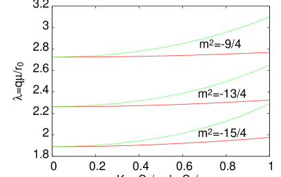
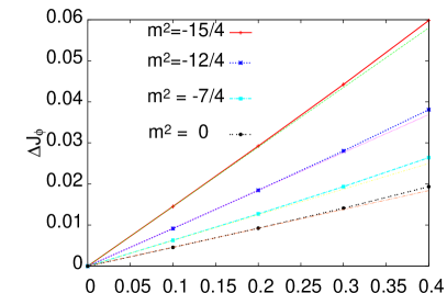
Figure 1: (left panel) The dependence of the critical chemical potential on the superflow parameter $S_{\phi}$. We plot $\lambda=q\mu/r_{0}$ vs. $K=qS_{\phi}/r_{0}$ (green, dashed curves) or the same spectral parameter vs. $k=S_{\phi}/\mu$ (red, solid curves), for $m^{2}$ equal to $-9/4,~{}-13/4,~{}-15/4$, respectively. One observes quadratic increase of $\lambda$ with $k$ and $K$, albeit on different scales. (right panel) The dependence of the super-current $\Delta J_{\phi}=(J_{\phi}-S_{\phi})/(q^{2}~{}S_{\phi}~{}<{\cal O}_{i}>^{2})$ in a s-wave superconductor on the velocity $S_{\phi}$, for a few values of the parameter $-4=m^{2}_{BF}<m^{2}\leq 0$ (curves with symbols). Curves without symbols correspond to linear approximations for low values of $S_{\phi}$.

2.2 Critical phenomena

In this subsection we shall concentrate on the relation connecting charge density and the chemical potential. Because of the fact that the equations describing the problem in question are the same as studied in nak15a , we refer the reader to this reference for the details.

Among all, one finds that the order parameter $<{\cal O}_{i}>$ depends on the chemical potential as

$$<{\cal O}_{i}>=\sqrt{\frac{{\tilde{\alpha}}~{}(\mu-\mu_{c})}{2~{}\mu_{c}~{}\xi(0)}}.$$ (35)

It shows that the critical phenomenon represents the second order phase transition for which the exponent has the mean field value $1/2$. The final result describing the dependence of $\rho$ on the chemical potential $\mu$ reads

$$\rho=\frac{\mu-\mu_{c}}{2~{}\xi(0)}~{}q^{2}~{}\int_{0}^{1}dz~{}z^{2\Delta_{i}-3}~{}F^{2}(z).$$ (36)

As in nak15 the charge density for s-wave holographic superfluid is proportional to the difference of $(\mu-\mu_{c})$ and is independent of $\alpha$-coupling constant of dark matter sector.

2.3 Behavior of $A_{\phi}$ near critical point

To extract the relation between the super-current $J_{\phi}$ and velocity $S_{\phi}$ one needs to consider the asymptotic behavior of $A_{\phi}$. Thus we investigate here the properties of $A_{\phi}$-component of Maxwell field near the critical point. The inspection of the equation of motion (19) reveals

$$A_{\phi}^{\prime\prime}-\frac{1}{z}A_{\phi}^{\prime}-\frac{2~{}q^{2}~{}z^{2\Delta_{i}}~{}<{\cal O}_{i}>^{2}~{}r_{0}^{2}~{}F^{2}(z)}{{\tilde{\alpha}}~{}f(z)~{}z^{4}}~{}A_{\phi}=0,$$ (37)

Then, expanding $A_{\phi}$ near the critical point in series, implies

$$A_{\phi}\simeq S_{\phi}(1-z^{2})+<{\cal O}_{i}>^{2}~{}\bigg{[}\kappa(0)+\kappa^{\prime}(0)~{}z+\frac{1}{2}~{}\kappa^{\prime\prime}(0)~{}z^{2}+\dots\bigg{]}.$$ (38)

The same procedure as in the preceding section implemented to $A_{\phi}$, enables us to find that for $\kappa(z)$ up to 2-order in $<{\cal O}_{i}>$, we get

$$\kappa^{\prime\prime}(z)-\frac{1}{z}~{}\kappa(z)^{\prime}\simeq\frac{2~{}q^{2}}{~{}r_{0}^{2}{\tilde{\alpha}}~{}f(z)}~{}S_{\phi}~{}(1-z^{2})~{}z^{2\Delta_{i}-4}~{}F^{2}(z).$$ (39)

In the next step we find that

$$\kappa^{\prime\prime}(0)=\frac{\kappa^{\prime}(z)}{z}\mid_{z\rightarrow 0}=-\frac{2~{}q^{2}~{}S_{\phi}}{~{}r_{0}^{2}}~{}\int_{0}^{1}dz~{}\frac{(1-z^{2})}{{\tilde{\alpha}}~{}f(z)}~{}z^{2\Delta_{i}-5}~{}F^{2}(z),$$ (40)

where we have used the fact that inspection of the z-order terms reveals that $\kappa^{\prime}(0)=0$.

All the above help us to determine that

$$A_{\phi}=S_{\phi}(1-z^{2})-\frac{q^{2}~{}S_{\phi}~{}<{\cal O}_{i}>^{2}}{~{}r_{0}^{2}{\tilde{\alpha}}}~{}z^{2}~{}\int_{0}^{1}dx~{}\frac{(1-x^{2})}{f(x)}~{}x^{2\Delta_{i}-5}~{}F^{2}(x).$$ (41)

The obtained relation is in accord with our boundary condition demand that $A_{\phi}(1)=0$, at the critical point. The $A_{\phi}$ is $\alpha$-coupling dependent. The bigger $\alpha$ one considers, the smaller value of the spatial component of Maxwell field we gain. Thus, the existence of dark matter sector diminishes the value of $A_{\phi}$, causing the increase of the superfluid current $J_{\phi}$. Using the asymptotic behavior of $A_{\phi}$ as given in (16), the current $J_{\phi}$ is provided by

$$J_{\phi}=S_{\phi}+\frac{q^{2}~{}S_{\phi}~{}<{\cal O}_{i}>^{2}}{r_{0}^{2}~{}{\tilde{\alpha}}}~{}\int_{0}^{1}dx~{}\frac{(1-x^{2})}{f(x)}~{}x^{2\Delta_{i}-5}~{}F^{2}(x).$$ (42)

The above equation shows that the current $J_{\phi}$ is linearly related to the velocity $S_{\phi}$. Small deviations are expected for the dependence of the integral on $S_{\phi}$. In the right panel of figure 1, the dependence of $\Delta J_{\phi}=(J_{\phi}-S_{\phi})/(q^{2}~{}S_{\phi}~{}<{\cal O}_{i}>^{2})$ on $S_{\phi}$ is shown for a s-wave superconductor and for a few values of the parameter $m^{2}_{BF}<m^{2}\leq 0$ and the coupling to the dark matter $\alpha=0$. Only the slight deviation from the linear dependence can be observed. It is traced back to the neglecting of backreaction effects. Due to independence of $<{\cal O}_{i}>^{2}/{\tilde{\alpha}}$ on $\alpha$ one notes that $J_{\phi}$ does not depend on dark matter.

3 Holographic p-wave superfluid model in soliton background

3.1 Vector model of p-wave superfluid

In this subsection we shall analyze the so-called Maxwell vector model of p-wave superfluids cai13 with dark matter sector. Its action is similar to the action appearing in quantum electrodynamical $\rho$-meson description dju05 .

The gravitational part of the model in question is the same as before, whereas the matter action is given by

$$S_{m}=\int\sqrt{-g}~{}d^{5}x\bigg{(}-\frac{1}{4}F_{\mu\nu}F^{\mu\nu} - \frac{1}{4}B_{\mu\nu}B^{\mu\nu}-\frac{\alpha}{4}~{}B_{\mu\nu}F^{\mu\nu}$$ (43)

$$-\frac{1}{2}~{}\rho^{\dagger}_{\mu\nu}~{}\rho^{\mu\nu} - m^{2}~{}\rho^{\dagger}_{\mu}~{}\rho^{\mu}+i~{}q~{}\gamma_{0}~{}\rho_{\mu}~{}\rho^{\dagger}_{\nu}~{}F^{\mu\nu}\bigg{)},$$

where $\rho_{\mu}$ is a complex vector field with mass $m$ and the charge $q$. The quantity $\rho_{\mu\nu}$ is defined by means of the co-variant derivative $D_{\mu}=\nabla_{\mu}-iqA_{\mu}$ in the form $\rho_{\mu\nu}=D_{\mu}\rho_{\nu}-D_{\nu}\rho_{\mu}.$ The last term in equation (43) is devoted to the magnetic moment of the vector field $\rho_{\mu}$. In the model under consideration, a charged $U(1)$ vector field is equivalent on the AdS/CFT side to an operator carrying the same charge under the symmetry in question. On the other hand, a vacuum expectation value of this operator is being subject to the spontaneous $U(1)$ symmetry breaking. The condensate of the dual operator leads to the $U(1)$ symmetry breaking. Due to vector character of the field, the rotational symmetry is broken by choosing a specific spatial direction. Therefore one can conclude that the vector field may be regarded as an order parameter and the model may describe p-wave superfluids.

We suppose that the vector field is real with only one component and the other gauge fields are chosen as

$$\rho_{\alpha}~{}dx^{\alpha}=\rho_{x}~{}dx,\qquad A_{\mu}~{}dx^{\mu}=\varphi(r)~{}dt+A_{\phi}(r)~{}d\phi,\qquad B_{\nu}~{}dx^{\nu}=\eta(r)~{}dt+\xi(r)~{}d\phi.$$ (44)

The close inspection of the equations of motion for the underlying theory with dark matter sector and with the real components of the vector field, gives us the same description as the s-wave model studied before, when we exchange $\psi(r)$ (which acts as an order parameter in s-wave case) for the $\rho_{x}$-component of the vector field. The same situation has been encountered earlier in the description of p-wave superconductors in rog16 . Therefore we shall not discuss this model and concentrate on the other holographic superfluid p-wave model, the $SU(2)$ one.

3.2 SU(2) Yang-Mills p-wave holographic superfluid model with dark matter sector

This section is devoted to the basic features of the SU(2) Yang-Mills holographic p-wave superfluid model with the dark matter sector. The action for the matter field is given by

$$S_{m}=\int\sqrt{-g}~{}d^{5}x\bigg{(}-\frac{1}{4}F_{\mu\nu}{}{}^{(a)}F^{\mu\nu(a)}-\frac{1}{4}B_{\mu\nu}{}{}^{(a)}B^{\mu\nu(a)}-\frac{\alpha}{4}~{}B_{\mu\nu}{}{}^{(a)}F^{\mu\nu(a)}\bigg{)},$$ (45)

where $F_{\mu\nu}{}{}^{(a)}$ and $B_{\mu\nu}{}{}^{(a)}$ are two $SU(2)$ Yang-Mills field strengths of the form $F_{\mu\nu}{}{}^{(a)}=\nabla_{\mu}A^{(a)}_{\nu}-\nabla_{\nu}A^{(a)}_{\mu}+\epsilon^{abc}~{}A^{(b)}_{\mu}A^{(c)}_{\nu}$. The totally antisymmetric tensor is set as $\epsilon^{123}=1$. The components of the gauge fields are bounded with the three generators $\tau$ of the $SU(2)$ algebra by the relations $A=A^{(a)}_{\beta}~{}\tau^{a}~{}dx^{\beta}$, where $[\tau^{a},~{}\tau^{b}]=\epsilon^{abc}~{}\tau^{c}$. As before, the parameter $\alpha$ describes the coupling between ordinary and dark matter $U(1)$-gauge fields.

The equations of motion for $B_{\mu\nu}$ are provided by

$$\nabla_{\mu}B^{\mu\nu(a)}+\frac{\alpha}{2}\nabla_{\mu}F^{\mu\nu(a)}+\epsilon^{abc}~{}B_{\mu}{}{}^{(b)}~{}B^{\mu\nu(c)}+\frac{\alpha}{2}\epsilon^{abc}~{}B_{\mu}{}{}^{(b)}~{}F^{\mu\nu(c)}=0.$$ (46)

and for $F_{\mu\nu}$ by

$$\nabla_{\mu}F^{\mu\nu(a)}+\frac{\alpha}{2}\nabla_{\mu}B^{\mu\nu(a)}+\epsilon^{abc}~{}A_{\mu}{}{}^{(b)}~{}F^{\mu\nu(c)}+\frac{\alpha}{2}~{}\epsilon^{abc}~{}A_{\mu}{}{}^{(b)}~{}B^{\mu\nu(c)}=0.$$ (47)

In order to simplify the above equations we multiply relation (46) by $\alpha/2$ and extract the term $\frac{\alpha}{2}\nabla_{\mu}B^{\mu\nu(a)}$. The second term in the equation (47) is replaced by the aforementioned outcome. The final result may be written as

$$\tilde{\alpha}~{}\nabla_{\mu}F^{\mu\nu(a)} - \frac{\alpha}{2}\epsilon^{abc}~{}B_{\mu}{}{}^{(b)}~{}B^{\mu\nu(c)}-\frac{\alpha^{2}}{4}\epsilon^{abc}~{}B_{\mu}{}{}^{(b)}~{}F^{\mu\nu(c)}$$

$$+ \epsilon^{abc}~{}A_{\mu}{}{}^{(b)}~{}F^{\mu\nu(c)}+\frac{\alpha}{2}\epsilon^{abc}~{}A_{\mu}{}{}^{(b)}~{}B^{\mu\nu(c)}=0,$$

where $\tilde{\alpha}=1-\frac{\alpha^{2}}{4}$.

Both $A_{\mu}{}{}^{(b)}$ and $B_{\mu}{}{}^{(b)}$ fields, are dual to some current operators in the four-dimensional boundary field theory. We choose the following components of the underlying gauge fields

$$A = \varphi(r)~{}\tau^{3}~{}dt+A_{\phi}(r)~{}\tau^{3}~{}d\phi+w(r)~{}\tau^{1}~{}dx,$$ (49)

$$B = \eta(r)~{}\tau^{3}~{}dt+\xi(r)~{}\tau^{3}~{}d\phi.$$ (50)

In the above relations the $U(1)$ subgroups of $SU(2)$ group generated by $\tau^{3}$ are identified with the electromagnetic $U(1)$-gauge field ($\varphi(r)$) and the other $U(1)$ group connected with the dark matter sector field ($\eta(r)$) coupled to the Maxwell one. The gauge boson field ($w(r)$) having the nonzero component along $x$-direction is charged under $A_{t}^{(3)}=\varphi(r)$. According to the AdS/CFT dictionary, $\phi(r)$ is dual to the chemical potential on the boundary, whereas $w(r)$ is dual to $x$-component of a charged vector operator. The condensation of $w(r)$ field will spontaneously break the $U(1)$ symmetry and is subject to the superconducting phase transition. It breaks the rotational symmetry by making the $x$-direction a special one and inclines the phase transition. The transition in question is interpreted as a p-wave superconducting phase transition on the boundary. As far as the $U(1)$-gauge field related to the dark matter sector is concerned, it has the component $B_{t}^{(3)}$ dual to a current operator on the boundary. One can remark that the choice described by the relation (49) is the only consistent choice of the gauge field components allowing the analytic treatment of the problem rog16 .

The direct calculations reveal that the $x(1)$, $\varphi(3)$ and $t(3)$ components of the equation (46) are given as follows

$$\frac{\alpha}{2}~{}\nabla_{\mu}F^{\mu x(1)} + \frac{\alpha}{2}~{}\bigg{(}\epsilon^{132}~{}B_{t}{}{}^{(3)}~{}F^{tx(2)}+\epsilon^{132}~{}B_{\varphi}{}{}^{(3)}~{}F^{\phi x(2)}\bigg{)}=0,$$ (51)

$$\nabla_{\mu}B^{\mu\phi(3)} + \frac{\alpha}{2}~{}\nabla_{\nu}F^{\nu\phi(3)}=0,$$ (52)

$$\nabla_{\mu}B^{\mu t(3)} + \frac{\alpha}{2}~{}\nabla_{\nu}F^{\nu t(3)}=0,$$ (53)

while the same components of the equation (47) yield

$$\nabla_{\mu}F^{\mu x(1)} + \epsilon^{132}~{}A_{\phi}{}{}^{(3)}~{}F^{\phi x(2)}+\epsilon^{132}~{}A_{t}{}{}^{(3)}~{}F^{tx(2)}=0,$$ (54)

$$\nabla_{\nu}F^{\nu\phi(3)} + \frac{\alpha}{2}~{}\nabla_{\nu}B^{\nu\phi(3)}+\epsilon^{312}~{}A_{x}{}{}^{(1)}~{}F^{xt(2)}=0,$$ (55)

$$\nabla_{\nu}F^{\nu t(3)} + \frac{\alpha}{2}~{}\nabla_{\nu}B^{\nu t(3)}+\epsilon^{312}~{}A_{x}{}{}^{(1)}~{}F^{\mu t(2)}=0,$$ (56)

and the main relation (3.2) reduces to the following:

$$\tilde{\alpha}~{}\nabla_{\mu}F^{\mu x(1)} - \frac{\alpha^{2}}{4}~{}\epsilon^{1bc}~{}B_{\mu}{}^{(b)}~{}F^{\mu x(c)}+\epsilon^{1bc}~{}A_{\mu}{}{}^{(b)}~{}F^{\mu x(c)}=0,$$ (57)

$$\tilde{\alpha}~{}\nabla_{\mu}F^{\mu\phi(3)} + \epsilon^{3bc}~{}A_{\mu}{}{}^{(b)}~{}F^{\mu\phi(c)}=0,$$ (58)

$$\tilde{\alpha}~{}\nabla_{\mu}F^{\mu t(3)} + \epsilon^{3bc}~{}A_{\mu}{}{}^{(b)}~{}F^{\mu t(c)}=0.$$ (59)

In what follows, we rewrite the above general equations for the adequate components of $A_{\mu}$ and $B_{\mu}$ gauge fields, given by the relations (49) and (50), discuss the appropriate boundary conditions, the asymptotic behavior and the relations between them in the superconducting and normal states.

3.2.1 Critical chemical potentials

As in s-wave case we shall consider the gravitational background of five-dimensional AdS soliton characterized by the line element (7)

$$ds^{2}=-r^{2}~{}dt^{2}+L^{2}~{}\frac{dr^{2}}{f(r)}+f(r)~{}d\phi^{2}+r^{2}~{}(dx^{2}+dy^{2}),$$ (60)

where $f(r)=r^{2}-r_{0}^{4}/r^{2}$. Let us recall that $r_{0}$ denotes the tip of the line element which constitutes a conical singularity of the considered solution. Solitonic background means that we shall consider zero temperature model of p-wave superfluid. In order to solve the underlying equations of motion for the p-wave holographic superfluid model, one imposes the adequate Neuman-like boundary conditions. At the tip one has the same boundary conditions as in the s-wave superfluid problem

$$w = w_{0}+w_{1}~{}(r-r_{0})+w_{2}~{}(r-r_{0})^{2}+\dots,$$ (61)

$$A_{\phi} = A_{\phi(0)}+A_{\phi(1)}(r-r_{0})^{2}+\dots,$$ (62)

$$\varphi = \varphi_{(0)}+\varphi_{(1)}~{}(r-r_{0})+\varphi_{(2)}~{}(r-r_{0})^{2}+\dots,$$ (63)

$$\eta = \eta_{(0)}+\eta_{(1)}(r-r_{0})+\eta_{(2)}(r-r_{0})^{2}+\dots,$$ (64)

$$\xi = \xi_{(0)}+\xi_{(1)}(r-r_{0})+\xi_{(2)}(r-r_{0})^{2}+\dots,$$ (65)

where $w_{j}$ $A_{\phi(j)},~{}\varphi_{(j)},~{}\eta_{(j)},~{}\xi_{(j)}$, for $j=0,~{}1,~{}2,\dots$ are constants. One encumbers the Neumann-like boundary condition to obtain every physical quantity finite nis10 . Contrary, near the boundary where $r\rightarrow\infty$, we have the different asymptotic behavior (comparing to the s-wave case). The asymptotic solutions read

$$w\rightarrow w_{0} + \frac{w_{2}}{r^{2}},\qquad\varphi\rightarrow\mu-\frac{\rho}{r^{2}},\qquad A_{\phi}\rightarrow S_{\phi}-\frac{J_{\phi}}{r^{2}},$$ (66)

$$\eta\rightarrow\mu_{D} - \frac{\rho_{D}}{r^{2}},\qquad B_{\phi}\rightarrow S_{D}-\frac{J_{D}}{r^{2}},$$ (67)

where $\mu,~{}\mu_{D}$ and $\rho,~{}\rho_{D}$ are interpreted as the chemical potential and the charge density in the dual theory for ordinary and dark matter, respectively. Similarly, $S_{\phi}$, $J_{\phi}$, $S_{D}$ and $J_{D}$ are interpreted as velocity and current of ordinary matter superfluid and dark matter sector quantities. Consequently with the requirements of the AdS/CFT dictionary, $w_{0}$ and $w_{2}$ have interpretations as a source and the expectation value of the dual operator. In order to gain the normalizable solution, one puts $w_{0}=0$ as we are interested in the spontaneous transitions to the condensed state.

In $z$-coordinates (with $r_{0}=1$) the equations in question yield

$$w^{\prime\prime}(z) + \bigg{(}\frac{f^{\prime}(z)}{f(z)}+\frac{1}{z}\bigg{)}~{}w^{\prime}(z)+\frac{\varphi(z)[\varphi(z)-\frac{\alpha^{2}}{4}~{}\eta(z)]}{\tilde{\alpha}~{}f(z)~{}z^{2}}~{}w(z)+$$

$$- \frac{A_{\phi}(z)[A_{\phi}(z)-\frac{\alpha^{2}}{4}~{}\xi(z)]}{\tilde{\alpha}~{}f^{2}(z)~{}z^{4}}~{}w(z)=0,$$

$$A_{\phi}^{\prime\prime}(z) - \frac{1}{z}~{}A_{\phi}^{\prime}(z)-\frac{w^{2}(z)}{\tilde{\alpha}~{}z^{2}~{}f(z)}~{}A_{\phi}(z)=0,$$ (69)

$$\varphi^{\prime\prime}(z) + \bigg{(}\frac{f^{\prime}(z)}{f(z)}+\frac{1}{z}\bigg{)}~{}\varphi^{\prime}(z)-\frac{w^{2}(z)}{\tilde{\alpha}~{}z^{2}~{}f(z)}~{}\varphi(z)=0.$$ (70)

The obtained equations can be benchmarked against the known results for SU(2) model of p-wave holographic superconductors. Putting ${\tilde{\alpha}}=1$ and $A_{\phi}=0$ one obtains the set of equations studied earlier in cai15 , albeit in 3+1 dimensional background. In analogy to the discussion of s-wave case we remark again, that it is a condensation of the field $w(z)$ which, when non-vanishing, couples various gauge fields and makes them linearly dependent everywhere in the bulk. On the other hand if, the vector condensate vanishes, $w(z)\equiv 0$, the various components of the gauge fields become independent.

In the next step we find the dependence of $\varphi(z)$ and $A_{\phi}(z)$ on the component of the dark matter sector $\eta(z)$ and $\xi(z)$. Using the the adequate components of the metric tensor for the line element (60) and the equations (52)-(53), we arrive at the following relations

$$\xi(z) + \frac{\alpha}{2}~{}A_{\phi}=C_{1}~{}(1-z^{2}),$$ (71)

$$\eta(z) + \frac{\alpha}{2}~{}\varphi(z)=D_{2},$$ (72)

where $C_{1}$ and $D_{2}$ are integration constants. The integration constant $D_{1}$ we put equal to zero at $z=0$, due to the well behavior of the functions. We set $D_{2}=\mu_{D}$. On the other hand, the relation between $C_{1}$ and $C_{2}$ was established taking into account the boundary conditions $\xi(1)=0$ and $A_{\phi}(1)=0$, then identify the integration constants with dark matter characteristics $S_{D}$ and $\mu_{D}$, one obtains

$$\xi(z) = S_{D}~{}(1-z^{2})-\frac{\alpha}{2}~{}A_{\phi}(z),$$ (73)

$$\eta(z) = \mu_{D}-\frac{\alpha}{2}~{}\varphi(z).$$ (74)

For $z$ close to boundary $z\rightarrow 0$, we use the fact that $\varphi(z)=\mu$ and $A_{\phi}=S_{\phi}(1-z^{2})$, which in turn leads to the following relations:

$$\xi(z) = S_{D}~{}(1-z^{2})-\frac{\alpha}{2}~{}S_{\phi}(z)(1-z^{2}),$$ (75)

$$\eta(z) = \mu_{D}-\frac{\alpha}{2}~{}\mu(z).$$ (76)

Let us turn back to the problem of the consistency of the chosen ansatz. Using the equation (51) and (54) multiplied by $\alpha/2$, as well as having in mind the relations (75) and (76), we arrive at

$$\bigg{(}-\frac{(2+\alpha)}{\alpha}~{}B_{\phi}{}{}^{(3)}+\frac{2}{\alpha}S_{D}~{}(1-z^{2})\bigg{)}~{}F^{\phi x(2)}+\bigg{(}-\frac{(2+\alpha)}{\alpha}~{}B_{t}{}{}^{(3)}+\frac{2}{\alpha}\mu_{D}\bigg{)}~{}F^{tx(2)}=0.$$ (77)

Having in mind that

$$F_{\phi x}{}{}^{(2)}=A_{\phi}{}{}^{(3)}A_{x}{}{}^{(1)},\qquad F_{tx}{}{}^{(2)}=-A_{x}{}{}^{(1)}A_{t}{}{}^{(3)},$$ (78)

we obtain the following relation binding the components of the ansatz if $A^{(1)}_{x}=w(z)\neq 0$

$$\bigg{(}-\frac{(2+\alpha)}{\alpha}~{}\xi(z)+\frac{2}{\alpha}S_{D}~{}(1-z^{2})\bigg{)}~{}A_{\phi}(z)~{}g^{\phi\phi}-\bigg{(}-\frac{(2+\alpha)}{\alpha}~{}\eta(z)+\frac{2}{\alpha}\mu_{D}\bigg{)}~{}\varphi(z)~{}g^{tt}=0.$$ (79)

This relation between $A_{\phi}(z)$ and $\phi(z)$ is valid for condensed state. On the other hand, for $A^{(1)}_{x}=0$ equation (77) is identically fulfilled and both components of $A_{\mu}$ evolve independently.

The above equations enable us to rewrite the equation (3.2.1) as

$$w^{\prime\prime}(z) + \bigg{(}\frac{f^{\prime}(z)}{f(z)}+\frac{1}{z}\bigg{)}~{}w^{\prime}(z)+\mu^{2}~{}\frac{[\beta-(1-\tilde{\alpha})k_{\mu}]}{\tilde{\alpha}}~{}\frac{1}{f(z)~{}z^{2}}~{}w(z)$$

$$- S^{2}_{\phi}(1-z^{2})^{2}~{}\frac{[\beta-(1-{\tilde{\alpha}})~{}k_{S}}{\tilde{\alpha}}~{}\frac{1}{f^{2}(z)~{}z^{4}}~{}w(z)=0,$$

where we have denoted by $k_{\mu}=\mu_{D}/\mu$ the ratio between chemical potentials of dark and visible sector, while by $k_{S}=S_{D}/S_{\phi}$ similar ratio of the velocities, $\beta=1+\alpha^{3}/8$. The obtained equation for the field $w(z)$ is valid close to the critical value of the chemical potential $\mu_{c}$ and in fact constitutes an equation for its determination. To find $\mu_{c}$, we correct the solution for $w(z)$ close to the boundary $z\rightarrow 0$ by defining the trial function $G(z)$

$$w(z)\sim<{\cal O}>~{}z^{2}~{}G(z),$$ (81)

with $G(z)=1-az^{2}$ fulfilling the appropriate boundary conditions $G(0)=1$ and $G^{\prime}(0)=0$ and $<{\cal O}>=w_{2}$. Equation for $w(z)$ can be rewritten in the form adequate to study the Sturm-Liouville eigenvalue problem sio10

$$(P(z)~{}G^{\prime}(z))^{\prime}-Q(z)~{}G(z)+{\Lambda}^{2}~{}R(z)~{}G(z)=0,$$ (82)

where we have defined

$$\Lambda^{2} = \mu^{2}~{}\frac{\beta-(1-\tilde{\alpha})k_{\mu}}{\tilde{\alpha}}$$ (83)

$$P(z) = z^{5}~{}f(z),$$ (84)

$$Q(z) = -f(z)~{}\bigg{(}4z^{3}+2z^{4}~{}\frac{f^{\prime}(z)}{f(z)}-S_{\phi}^{2}(1-z^{2})^{2}~{}\frac{[\beta-(1-{\tilde{\alpha}})~{}k_{S}]}{{\tilde{\alpha}}~{}f^{2}(z)}\bigg{)},$$ (85)

$$R(z) = z^{3}.$$ (86)

This equation allows us to find the minimum eigenvalue of $\Lambda^{2}$, by the method of minimizing the following functional with respect to $a$

$${\Lambda}^{2}=\frac{\int_{0}^{1}dz~{}[G^{\prime}(z)^{2}~{}P(z)+Q(z)~{}G^{2}(z)]}{\int_{0}^{1}dz~{}R(z)~{}G^{2}(z)}.$$ (87)

It has to be noted that the critical chemical potential $\mu_{c}$ we are looking at, depends on the parameters $k_{\mu}$ and $k_{S}$ as well as on the velocity $S_{\phi}$ and the $\alpha$-coupling constant to dark matter sector. Under the adopted approximations the dependence on $\mu_{c}(\alpha)$ has two sources: one is the direct dependence of $\Lambda(\alpha)$ and the other is subject to the function $Q(z)$, in the considered functional. The results are shown in the figures 2 and 3.

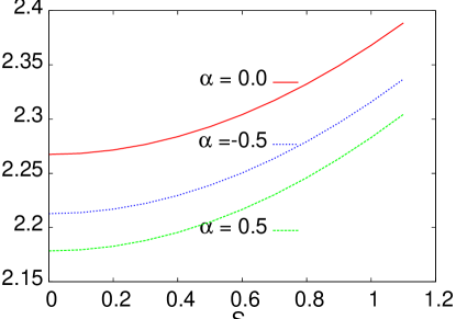
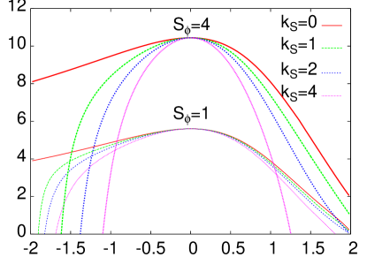
Figure 2: In the left panel we illustrate the dependence of the critical value of $\mu_{c}$ of the p-wave $SU(2)$ Yang-Mills superconductor on the velocity for a few values of the coupling constant $\alpha$, for fixed $\mu_{D}=S_{D}=0$. The right panel shows the dependence of the critical chemical potential squared on the coupling $\alpha$ to the dark matter, for $k_{\mu}=0$, two values of velocity $S_{\phi}=1,~{}4$ and a number of parameters $k_{S}=S_{D}/S_{\phi}$.

In view of the dependence of the critical chemical potential of the p-wave superfluid on four parameters ($\alpha$, $S_{\phi}$, $k_{S}$ and $k_{\mu}$), we shall only show some of the results. We start with the dependence of $\mu^{2}_{c}$ on the superfluid velocity $S_{\phi}$, for a few values of the $\alpha$-coupling to the dark matter sector and for $k_{S}=k_{\mu}=0$. The results are shown in the left panel of the figure 2.

The right panel of the figure 2 shows the dependence of $\mu^{2}_{c}$ on $\alpha$ for zero value of the dark matter chemical potential $\mu_{D}=0$, two values of the velocity $S_{\phi}=1,4$ and a few values of $k_{S}$ for each of the $S_{\phi}$. For some values of $\alpha$, the Sturm-Liouville eigenvalue $\Lambda$ drops below zero, which is unphysical. This means absence of the superconducting solution in these parameter ranges. Our equations are valid close to critical value of chemical potential, but otherwise are exact. The lack of the solution means that for those parameters, no matter how big will be the chemical potential, the system will stay insulating. The increase of the dark matter velocity $S_{D}$ ($k_{S}=S_{D}/S_{\phi}$) generally decreases the value of $\mu_{c}$ thus making the transition easier to appear, until one reaches zero value of $\mu_{c}$. This conclusion is generally true also for non-zero value of the dark matter chemical potential, as is visible in the right panel of the figure 3, albeit the detailed dependence $\mu_{c}(\alpha)$ is different. The fact that $\mu_{c}$ increases with the superflow $S_{\phi}$ indicates the adverse effect of the latter parameter on the transition.

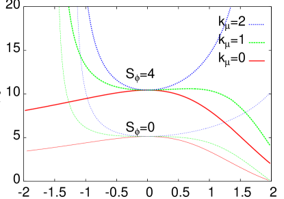
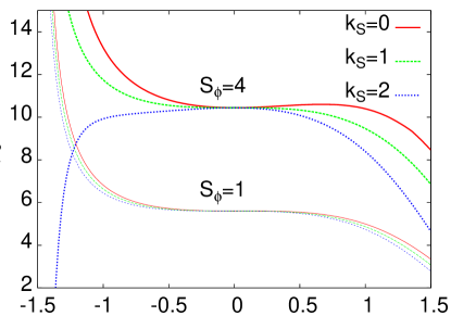
Figure 3: The dependence of the squared critical chemical potential on the $\alpha$-coupling to the dark matter, for $k_{\phi}=0$, a number of parameters $k_{\mu}=\mu_{D}/\mu_{c}$ and two values of superflow velocity $S_{\phi}=0,4$ (left panel). The right panel presents the similar dependence for $S_{\phi}=1,4$ and a few values of the velocity of dark matter parametrized by $k_{S}=S_{D}/S_{\phi}$ and for $k_{\mu}=1$. Note that the effect of the dark matter velocity is relatively small for the small values of $S_{\phi}$ and dramatically increases for the large values of the superflow.

The left panel of figure 3 envisages the dependence of $\mu_{c}^{2}$ on the $\alpha$-coupling constant of dark matter for $k_{S}=0$, a number of parameters $k_{\mu}=\mu_{D}/\mu_{c}$ and the two values of the superflow velocity $S_{\phi}=0,~{}4$. For a constant $\alpha\neq 0$, the growth of the dark matter chemical potential $\mu_{D}$ generally increases $\mu_{c}$, thus making the condensation harder to appear. The right panel of figure 3 shows the similar dependence of $\mu_{c}^{2}$ on $\alpha$ for $S_{\phi}=1,4$ and a few values of the velocity of dark matter parametrized by $k_{S}=S_{D}/S_{\phi}$ but contrary to the figure 2 for $k_{\mu}=1$. Note that the effect of the dark matter velocity is relatively small for small values of $S_{\phi}$ and dramatically increases for the elevated superflow. In the latter case the detailed behavior strongly depends on the dark matter velocity, $i.e.$, on $k_{S}$.

3.2.2 Critical phenomena in p-wave superfluid model

The equations of motion for $\varphi(z)$-component of the Maxwell field are the same as analyzed in rog16 , where holographic p-wave superconductor with dark matter sector have been studied. We refer the readers to this reference for the particulars of calculations and figures describing the elaborated quantities. However in this section we present only a bird eye view on the problem in question.

When $\mu\rightarrow\mu_{c}$, the condensate operator value is small but finite and the equation for time component of Maxwell potential is given by

$$\varphi^{\prime\prime}(z)+\bigg{(}\frac{f^{\prime}}{f}+\frac{1}{z}\bigg{)}~{}\varphi^{\prime}(z)-\frac{<{\cal O}>^{2}~{}z^{2}~{}F^{2}(z)}{\tilde{\alpha}~{}f}~{}\varphi(z)=0.$$ (88)

Calculations analogous to those presented previously in  rog16 lead to the following expression of the mean value of the condensation operator:

$$<{\cal O}>\simeq~{}\Delta~{}(\mu-\mu_{c})^{\frac{1}{2}},$$ (89)

where the pre-factor $\Delta=\sqrt{\frac{\tilde{\alpha}}{\mu_{c}\xi(0)}}$, the exact value of $\xi(0)$ is given in rog16 . The form of the equation (89) envisages the fact that the p-wave holographic superfluid critical phenomenon represents the second order phase transition for which the critical exponent has the mean field value $1/2$.

On the other hand, the charge density is found to linearly depend on $\mu$

$$\rho=(\mu-\mu_{c})~{}{\tilde{D}},$$ (90)

where the quantity $\tilde{D}$ is constant independent on $\alpha$.

3.2.3 $A_{\phi}$ in $SU(2)$ p-wave holographic model

In this subsection let us consider the velocity of p-wave superfluid current. The adequate equation of motion for the spatial component of Maxwell potential $A_{\phi}$ is given by

$$A_{\phi}^{\prime\prime}(z)-\frac{1}{z}~{}A_{\phi}^{\prime}(z)-\frac{w^{2}(z)}{\tilde{\alpha}~{}f(z)~{}z^{2}}~{}A_{\phi}(z)=0.$$ (91)

As in the preceding sections, we set again the ansatz for $w(z)=<{\cal O}>~{}z^{2}~{}F(z)$ and reduce the relation to the form

$$A_{\phi}^{\prime\prime}(z)-\frac{1}{z}~{}A_{\phi}^{\prime}(z)-\frac{<{\cal O}>^{2}~{}z^{2}~{}F^{2}(z)}{\tilde{\alpha}~{}f(z)}~{}A_{\phi}(z)=0.$$ (92)

The function $F(z)$ obeys the standard boundary conditions $F(0)=1,~{}F^{\prime}(0)=0$. To proceed further, let us approximate $A_{\phi}$ near the critical point. It yields

$$A_{\phi}\simeq S_{\phi}~{}(1-z^{2})+<{\cal O}>^{2}~{}\chi(z)+\dots$$ (93)

As in the previous case we expand $\chi(z)$, near the boundary of AdS space-time in a series provided by

$$\chi(z)=\chi(0)+\chi^{\prime}(0)z+\frac{1}{2!}~{}\chi^{\prime\prime}(0)z^{2}+\dots,$$ (94)

which leads to the relation of the form

$$\chi^{\prime\prime}(z)-\frac{1}{z}~{}\chi^{\prime}(z)=\frac{F^{2}(z)~{}z^{2}}{\tilde{\alpha}~{}f(z)}~{}(1-z^{2})~{}S_{\phi}(z)+{\cal O}\bigg{(}<{\cal O}>^{n\geq 2}\bigg{)}.$$ (95)

Then, the above equation can be rewritten in the form

$$(p(z)~{}\chi^{\prime}(z))^{\prime}+q(z)~{}F^{2}(z)=0,$$ (96)

where we have set

$$p(z)=\frac{1}{z},\qquad q(z)=-\frac{F^{2}(z)~{}z}{\tilde{\alpha}~{}f(z)}~{}(1-z^{2})~{}S_{\phi}.$$ (97)

Integrating the above relation and using the condition $\chi^{\prime}(0)=0$, one gains

$$\chi^{\prime\prime}(0)=\frac{\chi^{\prime}(z)}{z}\mid_{z\rightarrow 0}=-S_{\phi}\int_{0}^{1}dz~{}\frac{(1-z^{2})~{}z~{}F^{2}(z)}{\tilde{\alpha}~{}f(z)}.$$ (98)

Having in mind $z^{2}$-order terms, we can find that the superfluid current implies

$$J_{\phi}=S_{\phi}+S_{\phi}~{}\frac{<{\cal O}>^{2}}{\tilde{\alpha}}\int_{0}^{1}dz~{}\frac{(1-z^{2})~{}z~{}F^{2}(z)}{f(z)}~{}.$$ (99)

Consequently, the relation describing $A_{\phi}(z)$ yields

$$A_{\phi}(z)=S_{\phi}~{}(1-z^{2})-\frac{S_{\phi}~{}<{\cal O}>^{2}}{\tilde{\alpha}}~{}z^{2}~{}\int_{0}^{1}dx\frac{(1-x^{2})~{}F^{2}(x)}{f(x)}.$$ (100)

Taking into account the dependence of the pre-factor of $<{\cal O}>$ (see the equation (89)) on ${\tilde{\alpha}}$, one finds that the dark sector does not directly effect the current of holographic p-wave superconductor. Contrary to the s-wave case, the current depends on dark matter indirectly via $\mu_{c}=\mu_{c}(\alpha,\mu_{D},S_{D})$.

4 Holographic s-wave superfluid in black hole background

In this section we take up the problem of three dimensional s-wave holographic superfluid at a certain temperature. In order to scrutinize the question one analyzes the background of five-dimensional AdS black hole given by the line element

$$ds^{2}=-f(r)~{}dt^{2}+\frac{dr^{2}}{f(r)}+\frac{r^{2}}{L^{2}}~{}(dx^{2}+dy^{2}+dz^{2}),$$ (101)

where $f(r)=r^{2}/L^{2}-r_{+}^{4}/r^{2}L^{2}$. In what follows, without loss of generality we set $L=1$. The Hawking temperature for the black hole is equal to $T_{BH}=r_{+}/\pi$ and defines the temperature $T$ at the boundary. We assume that the non-zero components of the Maxwell fields are given by $A_{t}(r)=\phi(r),~{}A_{y}(r)$. The equations of motion read

$$\psi^{\prime\prime}(r) + \bigg{(}\frac{3}{r}+\frac{f^{\prime}}{f}\bigg{)}~{}\psi^{\prime}(r)-\bigg{(}\frac{m^{2}}{f(r)}-\frac{q^{2}~{}\phi^{2}(r)}{f^{2}(r)}+\frac{q^{2}~{}A^{2}_{y}(r)}{r^{2}~{}f(r)}\bigg{)}~{}\psi(r)=0,$$ (102)

$$\phi^{\prime\prime}(r) + \frac{3}{r}~{}\phi^{\prime}(r)-2~{}\frac{q^{2}~{}\psi^{2}(r)}{{\tilde{\alpha}}~{}f(r)}~{}\phi(r)=0,$$ (103)

$$A^{\prime\prime}_{y}(r) + \bigg{(}\frac{1}{r}+\frac{f^{\prime}}{f}\bigg{)}~{}A^{\prime}_{y}(r)-2~{}\frac{q^{2}~{}\psi^{2}(r)}{{\tilde{\alpha}}~{}r^{3}~{}f(r)}~{}A_{y}(r)=0,$$ (104)

where the prime denotes the derivative with respect to $r$-coordinate. We again note that the dependence between $\phi(r)$ and $A(r)_{\mu}$ is induced by the condensation of the $\psi(r)$ field.

The close inspection of the above relations envisages that in $z=r_{+}/r$-coordinates, they are given by

$$\psi^{\prime\prime}(z) + \bigg{(}\frac{f^{\prime}}{f}-\frac{1}{z}\bigg{)}~{}\psi^{\prime}(z)+\frac{q^{2}~{}\phi^{2}(z)}{r_{+}^{2}z^{4}~{}f^{2}(z)}~{}\psi(z)-\frac{q^{2}~{}A^{2}_{y}(z)}{~{}r_{+}^{2}z^{2}~{}f(z)}~{}\psi(z)-\frac{m^{2}}{z^{4}~{}f(z)}~{}\psi(z)=0,$$ (105)

$$\phi^{\prime\prime}(z) - \frac{1}{z}~{}\phi^{\prime}(z)-2~{}\frac{q^{2}~{}\psi^{2}(z)}{{\tilde{\alpha}}~{}f(z)~{}z^{4}}~{}\phi(z)=0,$$ (106)

$$A^{\prime\prime}_{y}(z) + \bigg{(}\frac{1}{z}+\frac{f^{\prime}}{f}\bigg{)}A^{\prime}_{y}(z)-2~{}\frac{q^{2}~{}\psi^{2}(z)}{{\tilde{\alpha}}~{}r_{+}^{3}~{}f(z)~{}z}~{}A_{y}(z)=0,$$ (107)

where now the prime is bounded with taking derivative with respect to $z$-coordinate. We have also denoted by $f(z)$ the relation

$$f(z)=~{}\bigg{(}\frac{1-z^{4}}{z^{2}}\bigg{)}.$$ (108)

4.1 Critical temperature for s-wave superfluids

For $T\rightarrow T_{c}$ the condensate is very small $\psi(z)\rightarrow 0$. The value of the horizon radius for the black hole with temperature $T_{c}$ is denoted by $r_{+c}$. The asymptotic boundary conditions, as $r$ tends to infinity, are the same as given by the equation (16), with the replacement of $A_{\phi}$ and $J_{\phi}$ by $A_{y}$ and $J_{y}$, respectively.

The equation (106) for the $\phi$ field near the critical point reduces to the relation

$$\phi^{{}^{\prime\prime}}(z)-\frac{\phi^{\prime}(z)}{z}\simeq 0,$$ (109)

which has the general solution of the form $\phi(z)=c_{1}+c_{2}z^{2}$. The boundary conditions imposed on Maxwell t-component gauge field $\phi(1)=0$, enable us to find that

$$\phi\simeq\rho r_{+c}^{-2}(1-z^{2}).$$

Consequently, the inspection of the spatial component of the Maxwell gauge field, near the critical temperature implies

$$A^{\prime\prime}_{y}(z)+\bigg{(}\frac{f^{\prime}}{f}+\frac{1}{z}\bigg{)}~{}A^{\prime}_{y}(z)\simeq 0,$$ (110)

with the condition $A_{y}(1)=0$, we get $A_{y}=S_{y}$. We are looking for the function $\psi(z)$ near the boundary $z\rightarrow 0$ of the considered spacetime. It is approximated by the expression

$$\psi(z)\mid_{z\rightarrow 0}=\frac{<{\cal C}>}{r^{\Delta}_{+}}~{}z^{\Delta}~{}F(z),$$ (111)

where we have to set $F(0)=1,~{}F^{\prime}(0)=0$. Finally, near the critical temperature one arrives at

$$F^{\prime\prime}(z) + F^{\prime}(z)~{}\bigg{[}\frac{2\Delta}{z}+\bigg{(}\frac{f^{\prime}}{f}-\frac{1}{z}\bigg{)}\bigg{]}+{\lambda}^{2}~{}\frac{(1-z^{2})^{2}}{f^{2}(z)~{}z^{4}}~{}F(z)+$$

$$+ F(z)~{}\bigg{[}\frac{\Delta~{}(\Delta-1)}{z^{2}}+\frac{\Delta}{z}~{}\bigg{(}\frac{f^{\prime}}{f}-\frac{1}{z}\bigg{)}-\frac{m^{2}}{z^{4}~{}f(z)}-\frac{q^{2}~{}S^{2}_{y}}{~{}r^{2}_{+}z^{2}~{}f(z)}\bigg{]}=0,$$

with the parameter $\lambda^{2}=\rho^{2}~{}q^{2}/~{}r^{6}_{+}$. Repeating the procedure leading to the Sturm-Liouville functional, we get

$${\lambda}^{2}=\frac{\int_{0}^{1}dz~{}[F^{\prime}(z)^{2}~{}p(z)+q(z)~{}F^{2}(z)]}{\int_{0}^{1}dz~{}r(z)~{}F^{2}(z)},$$ (113)

where the introduced functions are defined as

$$p(z) = z^{2\Delta-1}~{}f(z),$$ (114)

$$q(z) = -z^{2\Delta-1}~{}f(z)~{}\bigg{[}\frac{\Delta~{}(\Delta-1)}{z^{2}}+\frac{\Delta}{z}~{}\bigg{(}\frac{f^{\prime}}{f}-\frac{1}{z}\bigg{)}-\frac{m^{2}}{z^{4}~{}f(z)}-\frac{q^{2}~{}S^{2}_{y}}{~{}r^{2}_{+}~{}z^{2}~{}f(z)}\bigg{]},$$ (115)

$$r(z) = \frac{z^{2\Delta-5}}{f(z)}~{}q^{2}~{}(1-z^{2})^{2}.$$ (116)

Interestingly, the relation for ${\lambda}^{2}$ which serves as a condition for the critical temperature of the superconductor itself depends parametrically on the temperature of the considered black hole. This is a direct consequence of the fact that the Hawking black hole temperature $T_{BH}=r_{+}/\pi$ and ${\lambda}_{min}=\rho q/r^{3}_{+}$ enter the function $q(z)$ above. In order to find the transition temperature $T_{c}$, one ought to elaborate the self-consistent solution of the transcendental equation (113), as the critical temperature is related to ${\lambda}_{min}$ $via$ relation

$$T_{c}=(\rho)^{\frac{1}{3}}~{}\bigg{(}\frac{1}{\pi^{3}~{}{\lambda}_{min}}\bigg{)}^{\frac{1}{3}}.$$ (117)

with ${\lambda}_{min}$ depending on $T_{c}$. This behavior is characteristic to the superconductor carrying the current or superfluid with non-zero velocity of the condensate. Without superflow, $S_{y}=0$, one gets simple equation for $T_{c}$.

We have solved the resulting equation numerically in a self-consistent way. The results of the dependence of $T_{c}$ on $S_{y}$ for a number of $m^{2}$ values are presented in figure 4. The increase of the velocity results in the rise of the eigenvalue of the Sturm-Liouville problem and thus by the equation (117) to decrease of the superconducting transition temperature. Quantitatively it agrees with the known phenomenology of real superconductors.

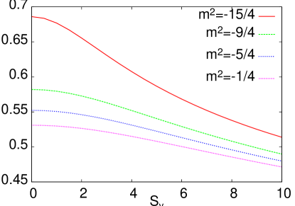
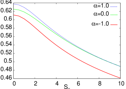
Figure 4: The dependence of the self-consistently calculated transition temperature of the current carrying superconductors of s-wave symmetry, equation (117) (left panel) and the p-wave symmetry, equation (148) (right panel), on the superflow velocity $S_{y}$ for a number of mass parameters $m^{2}$ or couplings $\alpha$, respectively. For numerical purposes we have taken $q=1$ and $\rho=1$. In the right panel we have set $k_{S}=0$ and $k_{\rho}=0$.

4.2 Condensation operator values

Here we study the influence of dark matter sector on the condensation operator for s-wave holographic superfluid. The equation of motion for $\phi$ is independent of the spatial component of the Maxwell field potential $A_{y}$ and has the form studied in nak15a . So we address here only the main features of the derivation, referring the reader the the previous work, for details.

The equation of motion for the time component of the Maxwell field, near the critical temperature is obtained from by introducing (111) into (106) and is given by

$$\phi^{\prime\prime}(z)-{\phi^{\prime}(z)\over z}={2~{}q^{2}~{}r_{+}^{2}~{}\phi(z)\over\tilde{\alpha}~{}f(z)}~{}z^{2\Delta-4}~{}\frac{<{\cal C}>^{2}}{r_{+}^{2\Delta}}~{}F^{2}(z).$$ (118)

Proceeding as in nak15a for $T\rightarrow T_{c}$, the condensation operator $<{\cal C}>$ is found as

$$<{\cal C}>=\sqrt{2~{}\tilde{\alpha}\over{\cal B}}~{}(\pi~{}T_{c})^{\Delta}~{}\sqrt{1-{T\over T_{c}}},$$ (119)

where ${\cal B}$ is given nak15a by

$${\cal B}=2\int_{0}^{1}dz~{}{q^{2}~{}r_{+}^{2}\over f(z)}~{}(1-z^{2})~{}z^{2\Delta-5}~{}F^{2}(z).$$ (120)

The mean value of the condensation operator depends on the $\alpha$-coupling constant of the dark matter sector. The bigger $\alpha$-coupling one takes into account, the smaller is the value of the condensate mean value operator $<{\cal C}>$. In addition operator $<{\cal C}>$ depends on $\alpha$ via $T_{c}(\alpha)$.

4.3 $A_{y}$ in s-wave superfluid at given temperature

Having in mind the relation (111) the equation of motion for $A_{y}(z)$ (107) near $T\rightarrow T_{c}$ reads

$$A^{\prime\prime}_{y}(z)+A^{\prime}_{y}(z)~{}\bigg{(}\frac{f^{\prime}}{f}+\frac{1}{z}\bigg{)}-\frac{2~{}q^{2}~{}A_{y}}{{\tilde{\alpha}}}<{\cal C}>^{2}~{}\frac{z^{2\Delta-1}~{}F^{2}(z)}{f(z)~{}r_{+}^{2\Delta+1}}\simeq 0.$$ (121)

To proceed further, we assume that

$$A_{y}(z)\simeq S_{y}+<{\cal C}>\chi(z),$$ (122)

and restrict our consideration to the terms of order $<{\cal C}>$. Consequently we obtain

$$\chi^{\prime\prime}(z)+\chi^{\prime}(z)~{}\bigg{(}\frac{f^{\prime}}{f}+\frac{1}{z}\bigg{)}-2\frac{q^{2}~{}<{\cal C}>~{}S_{y}}{{\tilde{\alpha}}~{}f(z)~{}r_{+}^{2\Delta+3}}~{}z^{2\Delta-1}~{}F^{2}(z)\simeq 0.$$ (123)

Like in the preceding sections, expansion of $\chi(z)$ in series near $z=0$ and the comparison of terms in the expansion of $z^{2}$-order, enable us to write the relation binding $A_{y}(z)$ and the super-current. It implies

$$A_{y}(z)=S_{y}-z^{2}~{}\frac{<{\cal C}>^{2}~{}S_{y}~{}q^{2}}{{\tilde{\alpha}}~{}r_{+}^{2\Delta+3}}~{}\int_{0}^{1}dx~{}x^{2\Delta}~{}F^{2}(x).$$ (124)

One can point out that, as in the AdS solitonic background the dark matter sector increases the value of the super-current $J_{y}(z)$, while its dependence on $S_{y}$ remains nearly linear in a close analogy to the s-wave superconductor in a solitonic background. On the other hand, the current does depend on the coupling constant to dark matter sector only through $T_{c}(\alpha)$, as is visible from the dependence of $<{\cal C}>^{2}\propto{\tilde{\alpha}}$. More importantly, we have found the dependence of the current on temperature in the linear form $J_{y}\propto(T_{c}-T)$, sometimes called the Onnes relation. This fact is in a significant contrast to the Ginzburg-Landau analysis of $J_{c}$ for thin superconducting films, i.e., effectively two-dimensional systems, were one has $J\propto(T_{c}-T)^{3/2}$. The experimental relevance of these results will be discussed later.

5 Holographic p-wave superfluid in black hole background

In this section we shall pay attention to the holographic p-wave superfluid case at finite temperatures. As in the previous sections, one can consider at least two models of p-wave holographic superfluids, i.e., the Maxwell vector and $SU(2)$ one. The same arguments as quoted in the section concerning holographic p-wave superfluid models in the AdS solitonic background, can be implemented in this case. Namely, the Maxwell vector model reduces to the s-wave case when one elaborates real vector field $\rho_{x}$. Therefore we restrict our considerations to the $SU(2)$ model. Taking into account five-dimensional AdS black hole background we choose gauge fields components as

$$A = \phi(r)~{}\tau^{3}~{}dt+A_{y}(r)~{}\tau^{3}~{}dy+w(r)~{}\tau^{1}~{}dx,$$ (125)

$$B = \eta(r)~{}\tau^{3}~{}dt+\xi(r)~{}\tau^{3}~{}dy.$$ (126)

The $z$-dependent equations of motion $x(1)$, $y(3)$ and $t(3)$ can be written as

$$w^{\prime\prime}(z) + \bigg{(}\frac{f^{\prime}(z)}{f(z)}+\frac{1}{z}\bigg{)}~{}w^{\prime}(z)+\frac{\phi(z)[\phi(z)-\frac{\alpha^{2}}{4}~{}\eta(z)]}{\tilde{\alpha}~{}f(z)~{}z^{2}}~{}w(z)+$$

$$- \frac{A_{y}(z)[A_{y}(z)-\frac{\alpha^{2}}{4}~{}\xi(z)]}{r_{+}^{4}~{}\tilde{\alpha}~{}f^{2}(z)~{}z^{4}}~{}w(z)=0,$$

$$A_{y}^{\prime\prime}(z) - \frac{1}{z}~{}A_{y}^{\prime}(z)-\frac{w^{2}(z)}{r_{+}^{2}~{}\tilde{\alpha}~{}z^{2}~{}f(z)}~{}A_{y}(z)=0,$$ (128)

$$\phi^{\prime\prime}(z) - \frac{1}{z}~{}\phi^{\prime}(z)-\frac{w^{2}(z)}{r_{+}^{2}~{}\tilde{\alpha}~{}z^{2}~{}f(z)}~{}\phi(z)=0,$$ (129)

where the prime denotes the derivative with respect to $z$-coordinate, $f(z)$ is described in the preceding section. The structure of the above equations is analogous to those studied earlier, with obvious changes related to the SU(2) character of the gauge field components. In particular their independence is lost due to the hairy structure, $w(z)\neq 0$, of the black hole. For $w(z)=0$, the equations (128) and (129) are independent and each of the components of the $A_{\mu}$ field evolves independently, albeit in the same way as it is visible from the above equations of motion.

The choice of the gauge field components (125) is the only consistent choice enabling the analytic considerations of the problem in question. The set of the differential equations (5)-(129) ought to be accomplished by the addition of the boundary conditions. One assumes that on the black hole event horizon $\phi(1)=0$ and the condensation field is of a finite norm, which in turn requires that $w(r_{+})$ should be finite. By virtue of the above, we assume that the following will hold in $r$ space

$$w = w_{0}+w_{1}~{}(r-r_{0})+w_{2}~{}(r-r_{+})^{2}+\dots,$$ (130)

$$A_{y} = A_{y(0)}+A_{y(1)}(r-r_{+})^{2}+\dots,$$ (131)

$$\phi = \phi_{(1)}~{}(r-r_{+})+\phi_{(2)}~{}(r-r_{+})^{2}+\dots,$$ (132)

$$\eta = \eta_{(0)}+\eta_{(1)}(r-r_{+})+\eta_{(2)}(r-r_{+})^{2}+\dots,$$ (133)

$$\xi = \xi_{(0)}+\xi_{(1)}(r-r_{+})+\xi_{(2)}(r-r_{+})^{2}+\dots,$$ (134)

where $w_{j}$ $A_{y(j)},~{}\phi_{(j)},~{}\eta_{(j)},~{}\xi_{(j)}$, for $j=0,~{}1,~{}2,\dots$ are constants. The Neumann-like boundary condition are required to obtain every physical quantity finite. When $r$ tends to infinity (one is close the boundary of the AdS space-time) the fields behave as

$$\phi(r)\rightarrow\mu-\frac{\rho}{r^{2}},\qquad w(r)\rightarrow w^{(0)}+\frac{w^{(2)}}{r^{2}},\qquad A_{y}(r)\rightarrow S_{y}-\frac{J_{y}}{r^{2}},$$ (135)

From equations

$$\nabla_{\mu}B^{\mu t(3)} + \frac{\alpha}{2}~{}\nabla_{\mu}F^{\mu t(3)}=0,$$ (136)

$$\nabla_{\mu}B^{\mu y(3)} + \frac{\alpha}{2}~{}\nabla_{\mu}F^{\mu y(3)}=0,$$ (137)

the dependence of $\phi(z)$ and $A_{y}(z)$ on the component of the dark matter sector $\eta(z)$ and $\xi(z)$ can be established. Namely, having in mind the boundary conditions $\eta(1)=0$ and $\phi(1)=0$ we can identify the integration constants with dark flow and dark density. It results in the following relations binding the ordinary and dark matter characteristics for the holographic p-wave superfluid

$$\xi(z) + \frac{\alpha}{2}~{}A_{y}=S_{D},$$ (138)

$$\eta(z) + \frac{\alpha}{2}~{}\phi(z)=\frac{\rho_{D}}{r^{2}_{+}}~{}(1-z^{2}).$$ (139)

For $z$ close to boundary, $z\rightarrow 0$, we use the fact that $\phi(z)=(\rho/r^{2}_{+})(1-z^{2})$ and $A_{y}(z)=S_{y}$ and rewrite the equation (5), having in mind the relations (138). Consequently it yields

$$w^{\prime\prime}(z) + w^{\prime}(z)\bigg{(}\frac{1}{z}+\frac{f^{\prime}}{f}\bigg{)}+\frac{1}{{\tilde{\alpha}}~{}z^{4}~{}f^{2}(z)}\bigg{(}\frac{\rho}{r^{3}_{+}}\bigg{)}^{2}(1-z^{2})^{2}~{}\bigg{[}\beta-(1-{\tilde{\alpha}})~{}k_{\rho}\bigg{]}w(z)$$

$$- \frac{~{}S_{y}^{2}}{r^{2}_{+}{\tilde{\alpha}}~{}z^{2}~{}f(z)}~{}\bigg{[}\beta-(1-{\tilde{\alpha}})~{}k_{S}\bigg{]}w(z)=0,$$

where we have defined

$$k_{S}=\frac{S_{D}}{S_{y}},\qquad k_{\rho}=\frac{\rho_{D}}{\rho}.$$ (141)

Inserting $w(z)\sim<{\cal R}>~{}z^{2}~{}G(z)$, we can rewrite the above equation in the form characteristic for studies of the Sturm-Liouville variational problem, which results in

$$G^{\prime\prime}(z) + \bigg{(}\frac{5}{z}+\frac{f^{\prime}}{f}\bigg{)}G^{\prime}(z)+\bigg{[}\frac{4}{z}+\frac{2}{z}\frac{f^{\prime}}{f}-\frac{~{}S_{y}^{2}}{r_{+}^{2}~{}{\tilde{\alpha}}~{}f(z)~{}z^{2}}~{}\bigg{(}\beta-(1-{\tilde{\alpha}})~{}k_{S}\bigg{)}\bigg{]}G(z)$$

$$+ \Lambda^{2}~{}\frac{(1-z^{2})^{2}}{f^{2}(z)~{}z^{4}}~{}G(z)=0,$$

where $\Lambda^{2}$ is provided by

$$\Lambda^{2}=\bigg{(}\frac{\rho}{r^{3}_{+}}\bigg{)}^{2}~{}[\beta-(1-{\tilde{\alpha}})~{}k_{\rho}].$$ (143)

The Sturm-Liouville variational problem enables us to achieve the minimum eigenvalue of $\Lambda^{2}$ from the functional

$$\Lambda^{2}=\frac{\int_{0}^{1}dz~{}[G^{\prime}(z)^{2}~{}p(z)+q(z)~{}G^{2}(z)]}{\int_{0}^{1}dz~{}r(z)~{}G(z)},$$ (144)

where we have defined the following quantities

$$p(z) = z^{5}~{}f(z),$$ (145)

$$q(z) = -z^{5}~{}f(z)~{}\bigg{[}\frac{4}{z^{2}}+\frac{2}{z}\frac{f^{\prime}}{f}-\frac{~{}S^{2}_{y}}{r_{+}^{2}{\tilde{\alpha}}~{}z^{2}~{}f(z)}~{}\bigg{[}\beta-(1-{\tilde{\alpha}})~{}k_{S}\bigg{]},$$ (146)

$$r(z) = \frac{z~{}(1-z^{2})^{2}}{f(z)}.$$ (147)

The transition temperature is calculated as

$$\pi T_{c}=\left(\frac{\rho^{2}[\beta-(1-{\tilde{\alpha}})~{}k_{\rho}]}{\Lambda^{2}}\right)^{1/6}.$$ (148)

In a close analogy to the s-wave superconductors discussed earlier, $T_{c}$ of the SU(2) p-wave superconductor has also to be determined in a self-consistent way, as the function $q(z)$ above depends on $r_{+}$ and makes $\Lambda$ to depend on $T_{c}$.

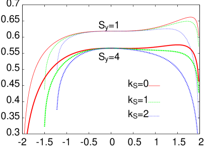
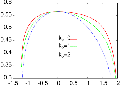
Figure 5: In the left panel we depicted the dependence of the self-consistently calculated transition temperature of the current carrying superconductor, equation (148), on the $\alpha$-coupling constant, for two values of the velocity $S_{y}=1,~{}4$, $k_{\rho}=0$ and a few values of the dark matter velocity $S_{D}$ parametrized here by $k_{S}=S_{D}/S_{y}$ is shown in the left panel. The right panel shows similar dependence of $T_{c}(\alpha)$ for $S_{y}=4$,  $k_{S}=2$ and three values of $k_{\rho}=0,1,2$.

The results of the self-consistent calculations of the $\alpha$ dependence of the transition temperature ($\pi T_{c}$) are shown in the left panel of figure 4 and in figure (5). For the current carrying superconductor $T_{c}$ is calculated form the relation (148). We show the results for $k_{\rho}=0$, two values of the superfluid velocity $S_{y}=1,~{}4$ and three values of the dark matter velocity $S_{D}$ parametrized here by $k_{S}=S_{D}/S_{y}$. With increasing dark matter velocity $T_{c}$ diminishes and eventually it ceases to exist (one gets negative solution for $\Lambda^{2}$) for negative values of $\alpha$. The behavior is qualitatively the same for both values of $S_{y}$. The right panel of figure 5 shows the similar dependence of $T_{c}(\alpha)$ for $S_{y}=4$,  $k_{S}=2$ and three values of $k_{\rho}=\rho_{D}/\rho=0,1,2$. The increase of the dark matter density generally leads to the relatively small decrease of $T_{c}$, for a given coupling $\alpha<0$ and larger decrease, for $\alpha$ closer to the value $2.$

5.1 Condensation value

In this subsection we discuss the behavior of the condensation operator due to the presence of dark matter sector and its dependence on temperature, near the critical one, $T_{c}$. The form of the equation (129) is the same as studied in rog16 , so for the details we refer to this work. For completeness of our discussion, we quote only the final result for the condensation operator $<{\cal R}>$

$$<{\cal R}>=\sqrt{\frac{2\tilde{\alpha}\pi^{2}}{E}}T_{c}(\alpha)\sqrt{1+\frac{T}{T_{c}(\alpha)}}~{}\sqrt{1-\frac{T}{T_{c}(\alpha)}},$$ (149)

where $E$ is given by the integral

$$E=\int_{0}^{1}dz~{}\frac{z^{3}~{}F^{2}(z)}{(1+z^{2})}.$$ (150)

One concludes that $<{\cal R}>$ depends on $\alpha$-coupling constant of the dark matter sector directly via factor $\tilde{\alpha}^{1/2}$ and indirectly through $T_{c}(\alpha)$. It also depends on the density $\rho_{D}$ of the dark matter via $T_{c}$. The mean value of the operator $<{\cal R}>$ can be interpreted as responsible for the pairing mechanism. The smaller vacuum expectation value it has, the harder condensation happens. So we conclude that dark matter sector destructively influences the condensation phenomena in p-wave superconductors for $\rho_{D}/\rho>1$. One has to notice, that in the presence of the velocity the dependence of $<{\cal R}>$ on $\alpha$ differs from that without super-flow and the resulting $\alpha$ dependence of $T_{c}$ will be different from that reported earlier rog16 .

5.2 $A_{y}$ in p-wave black hole holographic superfluid

As in the preceding sections we want to find the velocity and the current of the y-directed superflow. The equation of motion for $A_{y}(z)$ is of the form

$$A_{y}^{\prime\prime}(z)+\bigg{(}\frac{1}{z}+\frac{f^{\prime}}{f}\bigg{)}~{}A_{y}^{\prime}(z)-\frac{w^{2}(z)~{}A_{y}(z)}{r_{+}^{2}~{}{\tilde{\alpha}}~{}f(z)~{}z^{2}}=0.$$ (151)

For $T$ close to $T_{c}$ we correct $w(z)$ using an ansatz $w(z)=<{\cal R}>~{}z^{2}~{}F(z)$ and reduce the relation to the form

$$A_{y}^{\prime\prime}(z)+\bigg{(}\frac{1}{z}+\frac{f^{\prime}}{f}\bigg{)}~{}A_{y}^{\prime}(z)-\frac{<{\cal R}>^{2}~{}z^{2}~{}F^{2}(z)}{r_{+}^{2}~{}\tilde{\alpha}~{}f(z)}~{}A_{y}(z)=0.$$ (152)

To proceed, let us approximate $A_{y}(z)$ near the critical point by

$$A_{y}\simeq S_{y}+<{\cal R}>~{}\chi(z)+\dots$$ (153)

As in the previous cases we expand $\chi(z)$, near the boundary of AdS space-time in a series provided by

$$\chi(z)=\chi(0)+\chi^{\prime}(0)z+\frac{1}{2!}~{}\chi^{\prime\prime}(0)z^{2}+\dots,$$ (154)

which leads to the relation

$$\chi^{\prime\prime}(z)+\bigg{(}\frac{1}{z}+\frac{f^{\prime}}{f}\bigg{)}~{}\chi^{\prime}(z)=\frac{F^{2}(z)~{}z^{2}}{\tilde{\alpha}~{}f(z)}~{}(1-z^{2})~{}S_{y}(z)+{\cal O}\bigg{(}<{\cal R}>^{n\geq 2}\bigg{)}.$$ (155)

The above equation can be rewritten in the form

$$(p(z)~{}\chi^{\prime}(z))^{\prime}+q(z)~{}F^{2}(z)=0,$$ (156)

where we set for $p(z)$ and $q(z)$ the following relations:

$$p(z)=f(z)~{}z,\qquad q(z)=-\frac{<{\cal R}>~{}z^{3}}{r_{+}^{2}~{}\tilde{\alpha}}~{}S_{y}.$$ (157)

Integrating the above equation and using the condition $f(0)=0$, enable us to find that

$$\chi^{\prime\prime}(0)=\frac{\chi^{\prime}(0)}{z}\mid_{z\rightarrow 0}=-\frac{S_{y}}{r_{+}^{2}~{}}\int_{0}^{1}dz~{}\frac{z^{3}~{}F^{2}(z)}{\tilde{\alpha}}.$$ (158)

Thus we get

$$A_{y}(z)=S_{y}-\frac{S_{y}~{}<{\cal R}>^{2}}{2r_{+}^{2}~{}{\tilde{\alpha}}}~{}z^{2}~{}\int_{0}^{1}dx~{}x^{3}~{}F^{2}(x),$$ (159)

where the term multiplying $z^{2}$ is interpreted as the superfluid current. In analogy to the previously studied cases, the coupling constant to the dark matter sector cancels out and the current depends on $\alpha$ via transition temperature $T_{c}(\alpha)$ enters through $r_{+}$. Again, we find the linear in temperature, $(T_{c}-T)$ dependence, of the current. The disappearance of the current at $T=T_{c}$ is a well established behavior. It is encouraging that the holographic approach recovers this behavior.

6 Summary and discussion

In the paper we have considered the properties of holographic superfluid with the superflow of the condensate, i.e., the situation when on the gravity side one accepts not only t-component of the gauge fields but also takes into account the spatial one, as well. The problem in question has been studied analytically by means of the Sturm-Liouville variational method. We have analyzed the s-wave and p-wave current carrying superfluids with dark matter sector which has been described by additional $U(1)$-gauge field coupled to the ordinary one, in the background of the AdS soliton (T=0) or black hole (T$\neq$ 0). We have elaborated the probe limit case. According to the AdS/CFT dictionary the asymptotic ($r\rightarrow\infty$) behavior of the spatial component of the gauge potential $A_{\phi}(r)$, respectively $A_{y}(r)$, being of the form $A_{i}(r)=S_{i}-J_{i}/r^{2}$ are related to the superfluid velocity $S_{i}$ and superfluid current $J_{i}$ in the dual field theory.

In agreement with the previous analysis of the similar models without superflow we have found that the transitions are of the second order, as indicated by the mean field values of the critical exponents. The presence of the superflow does not change the fact that, neither the critical value of the chemical potential nor the density operator depend on $\alpha$-coupling constant. The spatial components of the Maxwell field identified with the currents at the boundary are affected by the coupling to dark matter sector. Also the current of the s-wave holographic superconductor in the solitonic background (equation (42)) does not depends on the dark matter sector. Its dependence on the chemical potential is of the form $J_{\phi}\propto(\mu-\mu_{c})$.

The critical chemical potential of the SU(2) p-wave holographic superconductor/superfluid in the solitonic background is strongly effected by the presence of dark matter. Not only it depends on the velocity of the condensate $S_{\phi}$ but also the coupling $\alpha$, the dark matter chemical potential $\mu_{D}$ and the dark matter velocity $S_{D}$. These dependencies have been illustrated in figures 2 and 3.

The black hole taken as a gravitational background allows the study of finite temperature phase transitions. The critical temperature of the model with superflow has to be calculated self-consistently, due to the transcendental character of the corresponding equations. This is true for both s-wave and p-wave symmetries. The s-wave superconducting transition temperature does not depend on the coupling constant to the dark matter sector. Contrary to that, the transition temperature of the p-wave SU(2) holographic superconductor depends on the dark matter not only $via$ the coupling $\alpha$ but also through the dark matter velocity $S_{D}$ and density $\rho_{D}$. In the figures, the last two parameters have been quantified by their ratio to corresponding parameters of the Maxwell sector.

In $SU(2)$ p-wave superfluids one can observe an interesting duality between solitonic and black hole backgrounds. Near $z\rightarrow 0$, in the case of solitonic background one has that $A_{\phi}$ is function of $z^{2}$ and $A_{t}$ tends to the constant value of chemical potential $\mu$. On the contrary, in black hole background the situation changes dramatically. The $t$-component is function of $z^{2}$, while the spatial one leads to the constant value of the superfluid velocity $S_{y}$.

The table I summarizes our findings related to the dependence on the dark matter of the critical chemical potentials, critical temperatures, the order parameters and the currents for both symmetries and both gravitational backgrounds, respectively. Of some interest are the universal relations of the currents on $\mu$, which read $J\propto(\mu-\mu_{c})$ for both s-wave and p-wave holographic superconductors. Much more important is the dependence of the currents on temperature. Again for both symmetries we get the linear in $(1-T/T_{c})$ dependence. This important finding which might be of relevance for real superconductors, as discussed below. In the literature, the above behavior is sometimes referred as the Onnes relation kvit15 ; dew01 .

Table 1: Summary of the obtained results. The table shows the functional dependence of the critical chemical potentials and temperatures as well as order parameters and currents of holographic superconductors on dark matter parameters $\alpha$, $\mu_{D}$ and $S_{D}$ (see text). Note the linear dependence of the currents on temperature for both symmetries of the order parameter independently of its symmetry.

	soliton (T=0)	black hole ($T\neq 0$)
	$\mu_{c}(\alpha)=\mu_{c}(0)$	$T_{c}=T_{c}(\alpha)$
s-wave	$<{\cal O}(\alpha)>=\sqrt{\tilde{\alpha}}<{\cal O}(0)>\propto(\mu-\mu_{c})$	$<{\cal O}(\alpha)>=\sqrt{\tilde{\alpha}}<{\cal O}(0)>$
	$J_{\phi}(\alpha)=J_{\phi}(0)(\mu-\mu_{c})$	$J_{y}(\alpha,T)=J_{y}(T_{c})(1-\frac{T}{T_{c}})$
	$\mu_{c}=\mu_{c}(\alpha,\mu_{D},S_{D})$	$T_{c}=T_{c}(\alpha,\mu_{D},S_{D})$
p-wave	$<{\cal O}(\alpha)>=\sqrt{\tilde{\alpha}}<{\cal O}(\mu_{c})>$	$<{\cal R}(\alpha)>=\sqrt{\tilde{\alpha}}<{\cal R}(T_{c})>$
SU(2)	$J_{\phi}(\alpha)=J_{\phi}(\mu_{c})(\mu-\mu_{c})$	$J_{y}(\alpha,T)=J_{y}(T_{c})(1-\frac{T}{T_{c}})$

Now we shall discuss the obtained results in the light of experimental data on different families of superconductors with various symmetries of the order parameter. We start with some preliminaries. It is well known that the vanishing of the electrical resistivity and the appearance of the ideal diamagnetism ($i.e.,$ the expulsion of the external magnetic field) below specific transition temperature $T_{c}$ are two defining characteristics of superconductors, with the latter being of utmost importance for the understanding of the phenomenon. The real material remains in the superconducting phase if its temperature $T$, magnetic field $B$ and the current (density) $J$ are kept below their critical values, $T_{c}$, $B_{c}$ or $J_{c}$, respectively. It means that on phase diagram in the temperature $T$, magnetic field $B$ and current $J$ space, there exist critical surface below which the system is superconducting. Out of the range of the aforementioned parameters, the changes of the superconducting properties of materials, subject to the current flow, are not quite well theoretically elaborated. However, it is known that if the current flowing in a superconductor exceeds a certain critical value, the system undergoes a superconductor to the normal metal transition.

The response of the superconductor to the current flow is completely different for the type I and type II superconductors, due to the appearance and the flow of vortices and the concomitant existence of two critical fields (lower and upper), in the latter. Generally it has been assumed that the superconductors undergo superconductor - normal conductor transition, if the flowing current produces on the surface of material magnetic field of the order of the critical one $H_{c}$ cyrot-pavuna . Type II superconductors are typically used for applications and they also can sustain only the finite currents. The maximum value of $J_{c}$ is related to the lower critical field $H_{c1}$ as indicated in recent experiments studying the properties of current currying superconductors tal15 ; tal16 ; kam16 , where some universalities observed in a number of different families of superconductors with various symmetries of the order parameter have been pointed out. Among all, it has been shown that for thin films of thickness $b$ less than the penetration depth $\lambda$, there exist a limiting value of the current $J_{c}$ which for type I superconductors is $H_{c}/\lambda$, whereas for type II materials $H_{c1}/\lambda$, where $H_{c1}$ is the lower critical field tal15 .

More recent data seem to indicate that the relation between $J_{c}$ and the penetration depth changes from $J_{c}\propto\lambda^{-3}$ valid for films with $b\leq\lambda$ to $J_{c}\propto\lambda^{-2}$ valid for films with $b>>\lambda$. This analysis which the main aim was to show the above dependence in the whole temperature range and for a number of different superconductors with various symmetries of the order parameter, obtained an additional support from the present ond earlier calculations using holography. Namely, the holographic analysis of (2+1)-dimensional superconductors and the present one studying 3+1 dimensional systems show universal temperature dependence of the currents for s-wave and p-wave superconductors of the form $J(T)=J(0)(1-T/T_{c})^{\nu}$ with the expenent $\nu$ depending only on the dimensionality of the system with $\nu=3/2$ for two dimensional and $\nu=1$ for three dimensional systems. The experimental data on three dimsional sample show kvit15 $J(T)=J(0)(1-T/T_{c})$ temperature dependence for $T$ close to $T_{c}$. For superconducting films of the thickness lower than the penetration depth, the experimental data for the critical current close to $T_{c}$ well agree with the dependence given by the relation $J(T)=J(0)(1-T/T_{c})^{3/2}$. Recent summary of a number of experimental data tal16 supports the holographic results.

- (1)
- (2)
- (3)
- (4) J.M.Maldacena, The large-N limit of superconformal field theories and supergravity, Adv. Theor. Math. Phys. 2 (1998) 231.
- (5) E.Witten, Anti-de-Sitter space and holography, Adv. Theor. Math. Phys. 2 (1998) 253.
- (6) S.S.Gubser, I.R.Klebanov and A.M.Polyakov, Gauge theory correlators from noncritical string theory, Phys. Lett. B 428 (1998) 105.
- (7) S.Sachdev, What can gauge-gravity duality teach us about condensed matter physics?, Annual Rev. of Cond. Matter Physics 3, (9) 2012.
- (8) M.Ammon and J.Erdmenger, Gauge/Gravity Duality, Cambridge University Press, Cambridge (2015).
- (9) Jan Zaanen, Ya-Wen Sun, Yan Liu and Koenraad Schalm, Holographic Duality in Condensed Matter Physics, Cambridge University Press, Cambridge (2015).
- (10) S.S.Gubser, Breaking an Abelian gauge symmetry near a black hole horizon, Phys. Rev. D 78 (2008) 065034.
- (11) S. S. Gubser, Colorful Horizons with Charge in Anti de Sitter Space, Phys. Rev. Lett. 101 (2008) 191601.
- (12) S.A.Hartnoll, C.P.Herzog and G.T.Horowitz, Building a holographic superconductor, Phys. Rev. Lett. 101 (2008) 031601.
- (13) G. T. Horowitz and M. M. Roberts, Holographic superconductors with various condensates, Phys. Rev. D 78 (2008) 126008.
- (14) K.Maeda and T.Okamura, Characteristic length of an AdS/CFT superconductor, Phys. Rev. D 78 (2008) 106006.
- (15) G. T. Horowitz, Introduction to holographic superconductors, in E. Papantonopoulos (ed.), From gravity to thermal gauge theories: the AdS/CFT correspondence, Lecture Notes in Physics, 821, Springer-Verlag, Berlin, Heidelberg 2011.
- (16) S.S.Gubser and S.S.Pufu, The gravity dual of a p-wave superconductor, JHEP 11 (2008) 033.
- (17) P.Basu, J.He, A.Mukharjee and H.H.Shieh, Hard-gapped holographic superconductors, Phys. Lett. B 689 (2010) 45.
- (18) F.Aprile, D.Rodriguez-Gomez and J.G.Russo, p-wave holographic superconductors and five-dimensional gauged supergravity, JHEP 01 (2011) 056.
- (19) S.Gangopadhyay and D.Roychowdhury, Analytic study of properties of holographic p-wave superconductors, JHEP 08 (2012) 104.
- (20) M.Ammon, J.Erdmenger, V.Grass and P.Kerner, On holographic p-wave superfluids with back-reaction, Phys. Lett. B 686 (2010) 192.
- (21) S.Liu, Y.Q.Wang, Holographic model of hybrid and coexisting s-wave and p-wave Josephson junction, Eur.Phys.J. C 75 (2015) 493.
- (22) J.W.Chen, Y.J.Kao, D.Maity, W.Y.Wen and C.P.Yeh, Towards a holographic model of D-wave superconductors, Phys. Rev. D 81 (2010) 106008.
- (23) F.Benini, C.P.Herzog, R.Rahman and A.Yarom, Gauge gravity duality for d-wave superconductors: prospects and challenges, JHEP 11 (2010) 137.
- (24) M.Rogatko and K.I.Wysokiński, Remarks on the Hall conductivity in chiral superconductors: weak vs. strong coupling approach, Acta Phys. Polonica A 126, (2014) A9.
- (25) H.B.Zeng, Z.Y.Fan and H.S.Zong, d-wave holographic superconductor vortex lattice and non-Abelian holographic superconductor droplet, Phys. Rev. D 82 (2010) 126008.
- (26) A.Amoreti, A.Braggio, N.Magiore, N.Magroll, and D.Musso, Coexistence of two vector order parameters: a holographic model for ferromagnetic superconductivity, JHEP 01 (2014) 054.
- (27) G.T.Horowitz and R.C.Myers, The AdS/CFT correspondence and a new positive energy conjecture for general relativity, Phys. Rev. D 59 (1998) 026005.
- (28) T.Nishioka, S.Ryu and T.Takayanagi, Holographic superconductor/ insulator transition at zero temperature, JHEP 03 (2010) 131.
- (29) R.G.Cai, H.F.Li, H.Q.Zhang, Analytical studies on holographic insulator/superconductor phase transitions, Phys. Rev. D 83 (2011) 126007.
- (30) A.Akhavan and M.Alishahiha, p-wave holographic insulator/superconductor phase transition, Phys. Rev. D 83 (2011) 086003.
- (31) Q.Pan, J.Jing and B.Wang, Analytical investigation of the phase transition between holographic insulator and superconductor in Gauss-Bonnet gravity, JHEP 11 (2011) 088.
- (32) R.G.Cai, S.He, L.Li and L.F.Li, A holographic study on vector condensate induced by a magnetic field, JHEP 12 (2013) 036.
- (33) L.Zhang, Q.Pan and J.Jing, Holographic p-wave superconductor models with Weyl corrections, Phys. Lett. B 743 (2015) 104.
- (34) P.Chaturvedi and G.Sengupta, p-wave holographic superconductors from Born-Infeld black holes, JHEP 04 (2015) 001.
- (35) R.G.Cai, Z.Y.Nie and H.Q.Zhang, Holographic phase transitions of p-wave superconductors in Gauss-Bonnet gravity with back-reaction, Phys. Rev. D 83 (2011) 066013.
- (36) R.G. Cai, L. Li, L. F. Li, R. Q. Yang, Science China - Phys Mech Astron 58, 060401 (2015)
- (37) Z.Zhao, Q.Pan and J.Jing, Holographic insulator/superconductor phase transition with Weyl corrections, Phys. Lett. B 719 (2013) 440.
- (38) J.Jing, Q.Pan and S.Chen, Holographic superconductor/insulator transition with logarithmic electromagnetic field in Gauss-Bonnet gravity, Phys. Lett. B 716 (2012) 385.
- (39) T.Albash and C.V.Johnson, A holographic superconductor in an external magnetic field, JHEP 09 (2008) 121.
- (40) X.H.Ge, B.Wang, S.F.Wu, and G.H.Yang, Analytical study on holographic superconductors in external magnetic field, JHEP 08 (2010) 108.
- (41) X.H.Ge and H.Q.Leng, Analytical Calculation on Critical Magnetic Field in Holographic Superconductor with Backreaction, Prog. Theor. Phys. 128 (1211) 2012.
- (42) S.L.Cui and Z.Xue, Critical magnetic field in a holographic superconductor in Gauss-Bonnet gravity with Born-Infeld electrodynamics, Phys. Rev. D 88 (107501) 2013.
- (43) D.Roychowdhury, Effect of external magnetic field on holographic superconductors in presence of nonlinear corrections, Phys. Rev. D 86 (106009) 2012.
- (44) C.P.Herzog, P.K.Kovtun, and H.H.Son, Holographic model of superfluidity, Phys. Rev. D 79 (2009) 066002.
- (45) P.Basu, A.Mukherjee, and H.H.Shieh, Supercurrent: Vector hair for an AdS black hole, Phys. Rev. D 79 (2009) 045010.
- (46) J.Sonner and B.Withers, Gravity derivation of the Tisza-Landau model in AdS/CFT, Phys. Rev. D 82 (2010) 026001.
- (47) D.Area, M.Bertolini, J.Evslin, and T.Prochazka, On holographic superconductors with DC current, JHEP 07 (2010) 060.
- (48) H.B.Zeng, W.M.Sun, and H.S.Zong, Supercurrent in a p-wave holographic superconductor, Phys. Rev. D 83 (2011) 046010.
- (49) H.B.Zeng, One dimensional -wave holographic superconductor with super-current, Phys. Rev. D 87 (2013) 046009.
- (50) D.Area, P.Basu, and TC.Krishnan, The many phases of holographic superfluids, JHEP 10 (2010) 006.
- (51) Y.B.Wu, J.W.Lu, W.X.Zhang, C.Y.Zhang, J.B.Lu, and F.Yu, Holographic p-wave superfluid, Phys. Rev. D 90 (2014) 126006.
- (52) Y.B.Wu, J.W.Lu, C.Y.Zhang, N.Zhang, X.Zhang, Z.Q.Yang, and S.Y.Wu, Lifshitz effects on holographic p-wave superfluid, Phys. Lett. B 741 (2015) 138.
- (53) M.Ammon, J.Erdmenger, M.Kaminski, and A.O’Bannon, Fermionic operator mixing in holographic p-wave superfluids, JHEP 05 (2010) 053.
- (54) I.Amado, D.Arean, A.Jimenez-Alba, K.Landsteiner, L.Melgar, and I.S.Landea, Holographic type II Goldstone bosons, JHEP 07 (2013) 108.
- (55) I.Amado, D.Arean, A.Jimenez-Alba, K.Landsteiner, L.Melgar, and I.S.Landea, Holographic superfluids and the Landau criterion, JHEP 02 (2014) 063.
- (56) C.Lai, Q.Pan, J.Jing, and Y.Wang, Analytical study on holographic superfluid in AdS solitonic background, Phys. Lett. B 757 (2016) 65.
- (57) P. Basu, J. He, A. Mukherjee and H.-H. Shieh, Superconductivity from D3/D7: holographic pion superfluid, JHEP 11, 070 (2009).
- (58) G.Hinshaw et al., Nine-year Wilkinson Microwave Anisotropy Probe (WMAP) observations, Astrophys. J. Suppl. Ser. 208 (2013) 19 .
- (59) P.A.R.Ade et al., astro-ph 1502.01589 (2015)Planck 2015 results. XIII. Cosmological parameters.
- (60) Ł.Nakonieczny and M.Rogatko, Analytic study on backreacting holographic superconductors with dark matter sector, Phys. Rev. D 90 (2014) 106004.
- (61) Ł.Nakonieczny, M.Rogatko and K.I. Wysokiński, Magnetic field in holographic superconductors with dark matter sector, Phys. Rev. D 91 (2015) 046007.
- (62) Ł. Nakonieczny, M. Rogatko and K.I. Wysokiński, Analytic investigation of holographic phase transitions influenced by dark matter sector, Phys. Rev. D 92 (2015) 066008.
- (63) M. Rogatko, K.I. Wysokiński, P-wave holographic superconductor/insulator phase transitions affected by dark matter sector, JHEP 03 (2016) 215.
- (64) M. Rogatko, K.I. Wysokiński, Holographic vortices in the presence of dark matter sector, JHEP 12 (2015) 041.
- (65) Y.Peng, Holographic entanglement entropy in superconductor phase transition with dark matter sector, Phys. Lett. B 750 (2015) 420.
- (66) Y.Peng, Q.Pan and Y.Liu, Holographic insulator/superconductor phase transition model with dark matter sector away from the probe limit, hep-th 1512.08950 (2015).
- (67) M.Regis, J.Q.Xia, A.Cuoso, E.Branchini, N.Fornengo, and M.Viel, Particle Dark Matter Searches Outside the Local Group, Phys. Rev. Lett. 114 (2015) 241301.
- (68) Y.Ali-Haimoud, J.Chluba, and M.Kamionkowski, Constraints on Dark Matter Interactions with Standard Model Particles from Cosmic Microwave Background Spectral Distortions, Phys. Rev. Lett. 115 (2015) 071304.
- (69) R.Foot and S.Vagnozzi, Dissipative hidden sector dark matter, Phys. Rev. D 91 (2015) 023512.
- (70) R.Foot and S.Vagnozzi, Diurnal modulation signal from dissipative hidden sector dark matter, Phys. Lett. B 748 (2015) 61.
- (71) J.Bramante and T.Linden, Detecting dark matter with imploding pulsars in the galactic center, Phys. Rev. Lett. 113 (2014) 191301.
- (72) J.Fuller and C.D.Ott, Dark-matter-induced collapse of neutron stars: a possible link between fast radio bursts and missing pulsar problem, Mon. Not. R. Astr. Soc. 450 (2015) L71.
- (73) I.Lopes and J.Silk, A particle dark matter footprint on the first generation of stars, Astrophys. J. 786 (2014) 25.
- (74) A.Nakonieczna, M.Rogatko, and R.Moderski, Dynamical collapse of charged scalar field in phantom gravity, Phys. Rev. D 86 (2012) 044043.
- (75) A.Nakonieczna, M.Rogatko, and L.Nakonieczny, Dark matter impact on gravitational collapse of an electrically charged scalar field, JHEP 11 (2015) 016.
- (76) Y.Brihaye and B.Hartmann Effect of dark strings on semi-local strings, Phys. Rev. D 80 (2009) 123502.
- (77) A.Geringer-Sameth and M.G.Walker, Indication of Gamma-Ray Emission from the Newly Discovered Dwarf Galaxy Reticulum II, Phys. Rev. Lett. 115 (2015) 081101.
- (78) K.Van Tilburg, N.Leefer, L.Bougas, and D.Budker, Search for Ultralight Scalar Dark Matter with Atomic Spectroscopy, Phys. Rev. Lett. 115 (2015) 011802.
- (79) P.Jean et al., Early SPI/INTEGRAL measurements of 511 keV line emission from the 4th quadrant of the Galaxy, Astron. Astrophys. 407 (2003) L55.
- (80) J.Chang et al., An excess of cosmic ray electrons at energies of 300-800 GeV, Nature 456, (2008) 362.
- (81) O.Adriani et al. (PAMELA Collaboration), An anomalous positron abundance in cosmic rays with energies 1.5-100 Gev, Nature 458, (2009) 607.
- (82) D.Harvey, R.Massey, T.Kitching, A.Taylor and E.Tittley, The nongravitational interactions of dark matter in colliding galaxy clusters, Science 347, (2015) 1462.
- (83) R.Massey et al., The behaviour of dark matter associated with four bright cluster galaxies in the 10 kpc core of Abell 3827, Mon. Not. R. Astr. Soc. 449 (2015) 3393.
- (84) G.W.Bennett et al., Final report of the E821 muon anomalous magnetic moment measurement at BNL, Phys. Rev. D 73 (2006) 072003.
- (85) A.Afanasev, O.K. Baker, K.B.Beard, G.Biallas, J.Boyce, M.Minarni, R.Ramdon, M.Shinn, and P.Slocum, New experimental limit on photon hidden-sector paraphoton mixing, Phys. Lett. B 679 (2009) 317.
- (86) S. N. Gninenko and J.Redondo, On search for EV hidden-sector in Supper-Kanionkande and CAST experiments, Phys. Lett. B 664 (2008) 180.
- (87) J.Suzuki, T.Horie, Y.Inoue, and M.Minowa, Experimental search for hidden photon CDM in the eV mass range with a dish antenna, JCAP 09, (2015) 042.
- (88) A.Mirizzi, J.Redondo, and G.Sigl, Microwave background constraints on mixing of photons with hidden photons, JCAP 03, (2009) 026.
- (89) J.Redondo and G.Raffelt, Solar constraints on hidden photons re-visited, JCAP 08, (2013) 034.
- (90) O.Domenech, M.Motull, A.Pomarol, A.Salvio, P.J.Silva, Emergent gauge fields in holographic superconductors, JHEP 08 (2010) 033.
- (91) T.Hertog and G.T.Horowitz, Towards a big crunch dual, JHEP 07 (2004) 073.
- (92) T.Hertog and G.T.Horowitz, Holographic description of AdS cosmologies, JHEP 04 (2005) 005.
- (93) G.Siopsis and J.Therrien, Analytic calculation of properties of holographic superconductors, JHEP 05 (2010) 013.
- (94) I.R.Klebanov and E.Witten, AdS/CFT correspondence and symmetry breaking, Nucl. Phys. B 556 (1999) 89.
- (95) D.Djukanovic, M.R.Schindler, J.Gegelia, and S.Scherer, Quantum electrodynamics for vector mesons, Phys. Rev. Lett. 95 (2005) 012001.
- (96) E. F. Talantsev, J. L. Tallon, Universal self-field critical current for thin-film superconductors, Nature Communications 6, (2015) 7820.
- (97) E. F. Talantsev, W. P. Crump and J. L. Tallon, Thermodynamic parameters of single- or multi-band superconductors derived from self-field critical currents, arXiv1609.03670v1 (2016).
- (98) A. Kaminski, S. Rosenkranz, M. R. Norman, M. Randeria, Z. Z. Li, H. Raffy, and J. C. Campuzano, Destroying Coherence in High-Temperature Superconductors with Current Flow, Phys. Rev. X 6 (2016) 031040.
- (99) J. Kvitkovic, R. Hatwar, S. V. Pamidi, S. Fleshler, C. Thieme, Temperature dependence of critical current and transport current losses of 4 mm YBCO coated conductors manufactured using nonmagnetic substrate, IOP Conf. Series: Materials Science and Engineering 102, (2015) 012033.
- (100) D. Dew-Hughes, The critical current of superconductors: an historical review, Fiz. Nizk. Temp. 27, (2001) 967, (Low Temp. Phys. 27, (2001) 713).
- (101) M. Cyrot, D. Pavuna, Introduction to Superconductivity and High- Materials, World Scientific (1992).