Boundary effects and gapped dispersion in rotating fermionic matter

Abstract

We discuss the importance of boundary effects on fermionic matter in a rotating frame. By explicit calculations at zero temperature we show that the scalar condensate of fermion and anti-fermion cannot be modified by the rotation once the boundary condition is properly implemented. The situation is qualitatively changed at finite temperature and/or in the presence of a sufficiently strong magnetic field that supersedes the boundary effects. Therefore, to establish an interpretation of the rotation as an effective chemical potential, it is crucial to consider further environmental effects such as the finite temperature and magnetic field.

1 Introduction

Examples of relativistic fermionic systems with substantial angular velocity are found in matter in extreme environments such as the cores of spinning compact stellar objects, the merger of binary stars, the heavy-ion collision, etc. In early days pioneering works [1, 2, 3] were motivated by astrophysical applications, and nowadays, the theoretical interest in relativistic rotating systems is being revived inspired by non-central collisions of heavy ions where a global spin polarization could be measurable [4, 5, 6, 7, 8, 9, 10, 11, 12]. Although it is technically difficult to design a directly rotating experiment, a material of Dirac/Weyl semimetal under circular polarized electromagnetic fields (as considered in Ref. [13] for instance) can be also understood in the same way as a rotating system, which is evident with an appropriate Floquet transformation [14]. From an intuitive analogy between the angular momentum and the magnetic field and a further formal similarity with Landau quantization-like effects [15, 16, 17], it has been anticipated that the rotation should induce as exotic phenomena as the magnetic field would do; one typical example is the topological current induced by vorticity (local rotation) [18, 19], which is called the chiral vortical effect and is analogous to the chiral magnetic effect [20, 21]. It is also pointed out that the chiral vortical effect has origins not only from the gauge sector but also from the gravitational (mixed) anomaly [22, 23]. These currents may affect some of the condensates and the ground state structure too [24].

For the magnetic effects on the ground state structure, the best known and understood is an inevitable formation of the scalar condensate leading to spontaneous breaking of chiral symmetry, which is referred to as the magnetic catalysis  [25, 26, 27, 28]. It is thus a quite natural idea to expect a rotational counterpart that affects some of the condensates. The question we are going to address is how the scalar condensate of fermion and anti-fermion (which will be called the “chiral condensate” hereafter) should be influenced by the rotation.

In a preceding work by two of the present authors and two colleagues [29], it has been demonstrated by explicit calculations that the rotation generates a term that can be interpreted as an effective chemical potential and such a masqueraded density manifests itself in a form of the finite-density inverse magnetic catalysis [30, 31] under a strong magnetic field. This finiteness of density is a genuine physical consequence beyond formal similarity and it arises from the quantum anomaly as argued in Ref. [32] (that is also closely related to the chiral pumping effect [13]) if a strong magnetic field is imposed.

Recently, a speculative scenario has been proposed about phase transitions caused solely by angular velocity [33]. Because the chiral condensate melts at sufficiently high density, it is likely that there is a critical value of the angular velocity, $\Omega_{c}$, above which the chiral condensate is vanishing. According to the estimate in Ref. [33] a first-order phase transition takes place at $\Omega_{c}\simeq 0.65\;\text{GeV}$ for rotating quark matter sitting at $r=0.1\;\text{GeV}^{-1}$ described by an effective model with four-fermion interaction. The purpose of this paper is to investigate the finite radius effects of rotating fermionic matter. In Ref. [33] the finite size effect has been partially taken into account in the local density approximation, but we will point out that not only the local information at $r$ but also the bulk boundary effects at $R$ would become as important.

Before looking into calculation details, let us give a hand-waving argument: The effective chemical potential in a rotating frame with $\boldsymbol{\Omega}=\Omega\hat{z}$ is characterized by $|\Omega j|$ where $j$ is the $z$-component of the total angular momentum. Therefore, fermionic modes with the energy lower than $|\Omega j|$ are Pauli blocked. If $\Omega$ goes larger, more modes are blocked and eventually formation of condensation could be hindered, which is an account for possible phase transitions unless the boundary effect is properly implemented. In finite size systems, the infrared (IR) cutoff is introduced and the momenta should be discrete. Hence, the fermion energy dispersion should have a gap of order of $\sim R^{-1}$. Because the wave-function with larger $j$ tends to have a more spreading configuration profile due to the centrifugal force, it costs a more energy in effect to confine the system in a cylinder, and accordingly the energy gap should also increase as $\sim R^{-1}|j|$. It would be then a delicate quantitative competition which of $|\Omega j|$ and $R^{-1}|j|$ can be larger. Our explicit calculations (at zero temperature) will show that the energy gap $\sim R^{-1}|j|$ is always larger than the effective chemical potential $|\Omega j|$, so that no mode is actually Pauli blocked. This means that the chiral condensate cannot be modified at all so long as the temperature is smaller than the effective chemical potential.

We append two brief comments about the above intuitive argument. First, we assume the quasiparticle approximation, which contains only the leading order contribution in the systematic expansion with respect to internal degrees of freedom (such as the number of the color of quarks). Since the contributions from the fermionic paired states (e.g. mesons) are the next higher order, the aforementioned argument is correct within the four fermion interaction model, which consists of the leading order terms. Besides even including bosonic states our argument should not to change because in the bosonic case the rotational energy shift cannot exceed the boundary gap, as discussed in Refs. [3, 34].

Second is about the difference of the rotational effects on fermions and antifermions. While the authentic chemical potential affects fermions and antifermions oppositely, the rotational energy shift influences fermions and antifermions similarly. Hence, both fermions and antifermions (and thus both $j>0$ and $j<0$ states) contribute to dynamics in rotating systems unlike the finite-density case at zero temperature. For example, if a fermion with angular momentum $j$ forms the chiral condensate, the partner antifermion should have $-j$ because the chiral condensate is a scalar paired state, with zero total angular momentum [33]. Therefore, in the Pauli blocking argument, as long as the authentic chemical potential is absent, fermions and antifermions and thus $j>0$ and $j<0$ states equally make a contribution and only the modulus of $\Omega j$ matters.

Our results imply that the phase transition scenario needs judicious refinements in the low-temperature region. At finite temperatures the situation could be qualitatively changed, because there is no strict Pauli blocking, and moreover the anomalous effects are turned on. In the end we will briefly mention on non-trivial interplay between the rotation and the finite temperature and magnetic field.

2 Reviewing the Dirac equation in a rotating frame

We explain our notation by making a quick summary of basic formulas for Dirac fermions in a rotating frame. The free Dirac equation in curved spacetime reads [35],

$$\bigl{[}i\gamma^{\mu}(\partial_{\mu}+\Gamma_{\mu})-m\bigr{]}\psi=0\;,$$ (1)

where the covariant derivatives associated with finite rotation are specified as $\Gamma_{\mu}=-\frac{i}{4}\omega_{\mu ij}\sigma^{ij}$ with the Dirac spin matrices $\sigma^{ij}=\frac{i}{2}[\gamma^{i},\gamma^{j}]$. The spin connection is given by $\omega_{\mu ij}=g_{\alpha\beta}e^{\alpha}_{i}(\partial_{\mu}e^{\beta}_{j}+\Gamma^{\beta}_{\mu\nu}e^{\nu}_{j})$ in terms of the metric and the vierbein, where Greek and Latin letters represent coordinate $(\mu=t,x,y,z)$ and tangent $(i=0,1,2,3)$ space, respectively. In a rotating frame with the angular frequency vector, ${\boldsymbol{\Omega}}=\Omega\hat{\boldsymbol{z}}$, we can write down the explicit form of the metric as

$$g_{\mu\nu}=\begin{pmatrix}1-(x^{2}+y^{2})\Omega^{2}&y\Omega&-x\Omega&0\\ y\Omega&-1&0&0\\ -x\Omega&0&-1&0\\ 0&0&0&-1\\ \end{pmatrix}\;.$$ (2)

The corresponding vierbein is not unique and for convenience we shall choose them as

$$e^{t}_{0}=e^{x}_{1}=e_{2}^{y}=e^{z}_{3}=1,\qquad e^{x}_{0}=y\Omega,\qquad e^{y}_{0}=-x\Omega\;,$$ (3)

and zero for the other components. We can simplify the Dirac matrix structure of Eq. (1) converting $\gamma^{\mu}$ to $\gamma^{i}$, and then the Dirac equation in these rotating $(t,x,y,z)$ coordinates with $\gamma^{i}$ takes the following form,

$$\Bigl{\{}i\gamma^{0}\bigl{[}\partial_{t}+\Omega(-x\partial_{y}+y\partial_{x}-\tfrac{i}{2}\sigma^{12})\bigr{]}+i\gamma^{1}\partial_{x}+i\gamma^{2}\partial_{y}+i\gamma^{3}\partial_{z}-m\Bigr{\}}\psi=0\;.$$ (4)

In this Dirac equation all the contributions with rotation are included in the effective chemical potential $\Omega(-x\partial_{y}+y\partial_{x}-\tfrac{i}{2}\sigma^{12})=\Omega\hat{J}_{z}$. This is not the case in hydrodynamic approaches; the vorticity is defined with derivative, and only the leading order term in the derivative expansion are usually picked up. The solutions of the above Dirac equation provide us a complete set of bases. The positive-energy particle solutions with positive and negative helicity take the following explicit form in the Dirac representation of $\gamma^{i}$’s;

$$u_{+}=\frac{e^{-iEt+ip_{z}z}}{\sqrt{\varepsilon+m}}\begin{pmatrix}\displaystyle(\varepsilon+m)\phi_{\ell}\\ \displaystyle 0\\ \displaystyle p_{z}\,\phi_{\ell}\\ \displaystyle ip_{\ell,\,k}\,\varphi_{\ell}\end{pmatrix},\;\;u_{-}=\frac{e^{-iEt+ip_{z}z}}{\sqrt{\varepsilon+m}}\begin{pmatrix}\displaystyle 0\\ \displaystyle(\varepsilon+m)\varphi_{\ell}\\ \displaystyle-ip_{\ell,\,k}\,\phi_{\ell}\\ \displaystyle-p_{z}\,\varphi_{\ell}\end{pmatrix},$$ (5)

where $\varepsilon\equiv|E+\Omega j|$. Here $j$ represents the $z$-component of the total angular momentum and we introduce $\ell=\ell_{+}=\ell_{-}-1$ with the azimuthal quantum number $\ell_{\pm}$ for spin “up” and “down” states, so that $j=\ell+1/2$ holds for any spin states. Also, we defined scalar functions of the radial momentum as $\phi_{\ell}=e^{i\ell\theta}J_{\ell}(p_{\ell,\,k}r)$ and $\varphi_{\ell}=e^{i(\ell+1)\theta}J_{\ell+1}(p_{\ell,\,k}r)$, which lead to the dispersion relation $\varepsilon^{2}=p_{\ell,\,k}^{2}+p_{z}^{2}+m^{2}$. In the same way the negative-energy antiparticle solutions with positive and negative helicity are obtained from $v_{\pm}=i\gamma^{2}u_{\pm}^{\ast}$ as

$$v_{+}=\frac{e^{iEt-ip_{z}z}}{\sqrt{\varepsilon+m}}\begin{pmatrix}\displaystyle-ip_{\ell,\,k}\,\varphi_{\ell}^{\ast}\\ \displaystyle-p_{z}\,\phi_{\ell}^{\ast}\\ \displaystyle 0\\ \displaystyle(\varepsilon+m)\phi_{\ell}^{\ast}\end{pmatrix},\;\;v_{-}=\frac{e^{iEt-ip_{z}z}}{\sqrt{\varepsilon+m}}\begin{pmatrix}\displaystyle-p_{z}\,\varphi_{\ell}^{\ast}\\ \displaystyle-ip_{\ell,\,k}\,\phi_{\ell}^{\ast}\\ \displaystyle-(\varepsilon+m)\varphi_{\ell}^{\ast}\\ \displaystyle 0\end{pmatrix}.$$ (6)

As we discuss later, we will compute the vacuum expectation value of field operators using these basis functions.

Lastly, we mention that our analysis with $u_{\pm}$ and $v_{\pm}$ is valid for the system with cylindrical symmetry. In a boundary without cylindrical symmetry (e.g. a rotating square), the angular momentum $\ell$ is no longer a good quantum number and thus the discussion based on the analytic calculation cannot be applied.

3 Momentum discretization

In a finite box the momenta should be discrete reflecting the (sharp) boundary condition imposed on the edge of the box. We now consider a cylinder that has a boundary at $r=\sqrt{x^{2}+y^{2}}=R$ and is infinitely long along the $z$-axis. Then, $p_{z}$ is not modified, while the radial momenta should take discrete values gapped by $\propto R^{-1}$, which was the reason why we denoted them as $p_{\ell,\,k}$. Since this discretization property is such crucial for our quantitative comparisons, let us carefully see how the discretization condition is physically required.

To this end, we see how the current conservation follows in a finite-size cylindrical system [36]. For the fermion in curved spacetime the vector current conservation law reads,

$$\nabla_{\mu}j^{\,\mu}=\frac{1}{\sqrt{|g|}}\partial_{\mu}(\sqrt{|g|}\,j^{\,\mu})=0\;,$$ (7)

where $\nabla_{\mu}$ represents the covariant derivative and $j^{\mu}=\bar{\psi}\gamma^{\mu}\psi$. Thus, to keep the total charge constant in a cylinder, we must impose a condition of no incoming flux at the spatial boundary as

$$\int_{V}dV\,\partial_{\alpha}(\sqrt{|g|}\;\bar{\psi}\gamma^{\alpha}\psi)\\ =\int_{\partial V}d\Sigma_{\alpha}\sqrt{|g|}\;\bar{\psi}\gamma^{\alpha}\psi=0\;.$$ (8)

Here $\alpha$ stands for the spatial components $x,y,z$ in coordinate space. In cylindrical coordinates the above condition turns into

$$R\int_{-\infty}^{\infty}dz\int_{0}^{2\pi}d\theta\;\bar{\psi}\gamma^{r}\psi\Bigr{|}_{r=R}=0\;.$$ (9)

We note that $\gamma^{r}\equiv\gamma^{1}\cos\theta+\gamma^{2}\sin\theta$ that follows from $\gamma^{1}\partial_{1}+\gamma^{2}\partial_{2}=\gamma^{r}\partial_{r}+r^{-1}\gamma^{\theta}\partial_{\theta}$. For arbitrary fermionic fields we can expand $\psi(x)$ using the complete set of $u_{\pm}(x)$ and $v_{\pm}(x)$, and then after the $\theta$-integration which constrains possible combinations of $\ell$, we find a superposition of four linear independent quantities;

$$\begin{split}&J_{\ell}(p_{\ell-1,k}R)J_{\ell}(p_{\ell,k^{\prime}}R)\;,\quad J_{\ell}(p_{\ell,k}R)J_{\ell}(p_{\ell-1,k^{\prime}}R)\;,\\ &J_{\ell}(p_{\ell-1,k}R)J_{\ell}(p_{-\ell-1,k^{\prime}}R)\;,\quad J_{\ell}(p_{\ell,k}R)J_{\ell}(p_{-\ell,k^{\prime}}R)\;.\end{split}$$

To realize the fluxless condition for arbitrary $\psi(x)$ we have to make all of them vanishing and this is possible when the transverse momenta are discretized as [36, 37]

$$p_{\ell,\,k}=\begin{cases}\xi_{\ell,\,k}\;R^{-1}\quad\text{for}\quad\ell=0,1,\dots\\ \xi_{-\ell-1,\,k}\;R^{-1}\quad\text{for}\quad\ell=-1,-2,\dots\end{cases}$$ (10)

where $\xi_{\ell,\,k}$ represents the $k$-th zero of $J_{\ell}(x)$.

The most fundamental quantity to calculate physical observables is Green’s function or the propagator. The propagator for rotating systems is modified by the boundary effects at $r=R$ as well as the non-trivial metric tensor involving $\Omega$. We can readily construct the free propagator from $u_{\pm}(x)$ and $v_{\pm}(x)$ as

$$\begin{split}S_{F}^{\alpha\beta}(x,x^{\prime})&=i\int\frac{dp_{0}\,dp_{z}}{(2\pi)^{2}}\frac{1}{2\pi}\sum_{\ell=-\infty}^{\infty}\sum_{k=1}^{\infty}\frac{2}{[J_{\ell+1}(p_{\ell,k}R)]^{2}R^{2}}\\ &\qquad\times\frac{e^{-ip^{0}(t-t^{\prime})+ip_{z}(z-z^{\prime})}}{(p^{0}+\Omega j)^{2}-\varepsilon^{2}+i\epsilon}\mathcal{S}^{\,\alpha\beta}(p;r,\theta,r^{\prime},\theta^{\prime})\;.\end{split}$$ (11)

We should note that the weight in the $\ell$- and $k$-sum are determined from the Bessel-Fourier expansion and the following orthogonal relation,

$$\int_{0}^{R}dr\,r\,J_{\ell}(p_{\ell,k}r)J_{\ell}(p_{\ell,k^{\prime}}r)=\frac{R^{2}}{2}\delta_{kk^{\prime}}[J_{\ell+1}(p_{\ell,k}R)]^{2}\;,$$ (12)

and we can numerically verify that the following approximation works at excellent precision for not too large $\ell$ (for example, for $\ell\sim 100$ and $k\sim 10$, the deviation is $\sim 1\%$ and the agreement is better for smaller $\ell$);

$$\frac{2}{[J_{\ell+1}(p_{\ell,k}R)]^{2}R^{2}}\approx p_{\ell,k}\,\Delta p_{\ell,k}\;,$$ (13)

where $\Delta p_{\ell,\,k}\equiv p_{\ell,\,k+1}-p_{\ell,\,k}$. This approximated form is useful to think of the continuum limit with $R\to\infty$. Using new notations, $\phi_{\ell}(r,\theta)\equiv\phi_{\ell}$, $\phi_{\ell}(r^{\prime},\theta^{\prime})\equiv\phi^{\prime}_{\ell}$ and so on, we can parametrize the matrix elements in the propagator as

$$\mathcal{S}(p;r,\theta,r^{\prime},\theta^{\prime})=\begin{pmatrix}\mathcal{M}_{+}&\mathcal{N}_{+}\\ \mathcal{N}_{-}&\mathcal{M}_{-}\end{pmatrix}\;,$$ (14)

with

$$\mathcal{M}_{\pm} \equiv\begin{pmatrix}(\pm p_{0}+m)\phi_{\ell}\phi^{\prime}_{\ell}&0\\ 0&(\pm p_{0}+m)\varphi_{\ell}\varphi^{\prime}_{\ell}\end{pmatrix}$$ (15)

$$\mathcal{N}_{\pm} \equiv\begin{pmatrix}-p_{z}\phi_{\ell}\phi^{\prime}_{\ell}&\pm ip_{\ell,k}\phi_{\ell}\varphi^{\prime}_{\ell}\\ \mp ip_{\ell,k}\varphi_{\ell}\phi^{\prime}_{\ell}&p_{z}\varphi_{\ell}\varphi^{\prime}_{\ell}\end{pmatrix}\;,$$ (16)

4 Rotating and yet unchanged condensate

Let us take an explicit example to calculate the field expectation value in the rotating frame. An effective model with four-fermion interaction is an ideal setup for this purpose to investigate the fate of the chiral condensate. The effective Lagrangian is

$$\mathcal{L}_{\text{4-fermi}}=\bar{\psi}\bigl{[}i\gamma^{\mu}(\partial_{\mu}+\Gamma_{\mu})-m\bigr{]}\psi+\frac{G}{2}\bigl{[}(\bar{\psi}\psi)^{2}+(\bar{\psi}i\gamma^{5}\psi)^{2}\bigr{]}\;.$$ (17)

The effective action at the one-loop order in the mean-field approximation reads,

$$\Gamma_{\text{eff}}[m(r)]=\int d^{4}x\,\frac{m(r)^{2}}{2G}-\text{Tr}\ln\bigl{[}\partial_{\mu}+\Gamma_{\mu}-m(r)\bigr{]}\;.$$ (18)

From the condition, $\delta\Gamma_{\text{eff}}[m]/\delta m(r)=0$, we can write down the gap equation as

$$m(r)=G\,\text{tr}\,S_{F}(x,x)\;.$$ (19)

Here $S^{\alpha\beta}_{F}(x,y)$ represents the free fermion propagator with mass $m(r)$. It is technically difficult to solve this functional gap equation self-consistently [38], and in the present work we will work in the local density approximation [33]. That is, we solve $m(r)$ at each $r$ as if $m(r)$ were an $r$-independent variable. We can justify such an approximate treatment for $\partial_{r}m\ll m^{2}$. Now under this approximation, we can perform the one-loop integration of the gap equation as

$$\begin{split}\frac{m(r)}{G}=\frac{i}{(2\pi)^{2}}\int_{-\infty}^{\infty}dp_{z}&\sum_{\ell=-\infty}^{\infty}\sum_{k=1}^{\infty}\frac{2}{[J_{\ell+1}(p_{\ell,k}R)]^{2}R^{2}}\\ &\times\int_{-i\infty+\Omega j}^{i\infty+\Omega j}\frac{dp_{0}}{2\pi}\frac{\text{tr}[\mathcal{S}(p;r,\theta)]}{p_{0}^{2}-\varepsilon^{2}}\;.\end{split}$$ (20)

We can explicitly take $\text{tr}[\mathcal{S}(p,r,\theta)]$ to simplify the right-hand side. We note that $\mathcal{S}(p,r,\theta)$ generally has the $\theta$-dependence, but its trace does not depend on $\theta$ any more as seen from

$$\text{tr}[\mathcal{S}(p,r,\theta)]=2m\bigl{[}J_{\ell}(p_{\ell,\,k}r)^{2}+J_{\ell+1}(p_{\ell,\,k}r)^{2}\bigr{]}\;.$$ (21)

Then, after the $p_{0}$-integration, the gap equation in the local density approximation leads to

$$\begin{split}\frac{m}{G}=\frac{m}{(2\pi)^{2}}\int_{-\infty}^{\infty}&dp_{z}\sum_{\ell=-\infty}^{\infty}\sum_{k=1}^{\infty}\frac{2}{[J_{\ell+1}(p_{\ell,k}R)]^{2}R^{2}}\\ &\times\frac{J_{\ell}(p_{\ell,\,k}r)^{2}+J_{\ell+1}(p_{\ell,\,k}r)^{2}}{\varepsilon}\theta\,\bigl{(}\varepsilon-|\Omega j|\bigr{)}\;.\end{split}$$ (22)

In the same way as the finite-density system, the effect of the rotation appears only in the form of the theta function constraint which represents an effective chemical potential of $|\Omega j|=|\Omega(\ell+1/2)|$ induced by rotation. Therefore, the modification caused by rotation comes out from the contribution with $\varepsilon<|\Omega j|$. Here we note that $m(r)$ has been assumed to be independent of $\Omega$, but we can confirm this self-consistently.

If we make an approximation of $R\sim\infty$ and treat the problem with a continuous transverse momentum instead of $p_{\ell,\,k}$, the rotation and the finite chemical potential appear identical in the gap equation. In a rotating frame, however, the causality constraint, $\Omega R\leq 1$, prevents us from taking arbitrarily large $R$. Once the boundary at $r=R$ is properly taken into account, there is no such mode that satisfies $\varepsilon<|\Omega j|$, as we see below. It is easy to understand this from the discretization condition; $\varepsilon$ becomes minimized at $p_{z}=m=0$ and $k=1$, so that we can see, for $\ell\geq 0$,

$$\varepsilon-\Omega|\ell+1/2| \geq\frac{1}{R}\Bigl{[}\xi_{\ell,\,1}-\Omega R(\ell+1/2)\Bigr{]}$$

$$\geq\frac{1}{R}\Bigl{[}\xi_{\ell,\,1}-(\ell+1/2)\Bigr{]}>0\,,$$ (23)

where we used the causality constraint $\Omega R\leq 1$ and an inequality known for the zeros of the Bessel function, that is [39],

$$\xi_{\ell,\,1}>\ell+1.855757\ell^{1/3}+0.5\ell^{-1/3}\qquad(\ell\geq 1)\;,$$ (24)

from which we can show $\xi_{\ell,\,1}>\ell+1/2>0$ for $\ell\geq 1$ and also we can check $\xi_{\ell,\,1}=2.40483>1/2$ for $\ell=0$. In the same way we can also prove that $\varepsilon<|\Omega j|$ is never realized for $\ell<0$. We note that a similar discussion is applicable to bosonic systems; $\varepsilon-|\Omega\ell|>0$ (for zero-spin bosons). This ensures that the bosonic thermal distribution in a rotating frame, $[e^{\beta(\varepsilon-\Omega\ell)}-1]^{-1}$ does not exhibit instability (see, for example, discussions in Ref. [34]).

Now we expect that the analogy between density and rotation could help us to clarify the above physics. In finite density systems microscopic quantities, such as the Dirac eigenvalue, are affected by chemical potential. The density effect on macroscopic quantities at zero temperature can however be visible only for the chemical potential lager than the mass threshold; this is well-known as the Silver Blaze problem in finite density QCD. Since rotation seems to generate the alignment of the azimuthal angular momentum and spin of each rotating fermion, the pairing state with zero total angular momentum might no longer be energetically most favored. Contrary to such an intuitive picture, as we have discussed above, the effective chemical potential $|\Omega j|$ can never exceed the threshold $p_{\ell,\,1}$.

Even though there is no rotation effect at zero temperature, it is an intriguing question how $m(r)$ looks like in the local density approximation with the boundary condition. To solve the gap equation (22) we need to introduce a ultraviolet (UV) regulator, which is a part of the four-fermion interacting model that is non-renormalizable. We do this by inserting a smooth cutoff function into the summation as follows;

$$f(p\,;\Lambda)=\frac{\sinh(\Lambda/\delta\Lambda)}{\cosh[\tilde{\varepsilon}(p)/\delta\Lambda]+\cosh(\Lambda/\delta\Lambda)}$$ (25)

with $\tilde{\varepsilon}\equiv\sqrt{p_{\ell,\,k}^{2}+p_{z}^{2}}$. This function is suppressed for $\tilde{\varepsilon}>\Lambda$ and the suppression smoothness is tuned by a parameter $\delta\Lambda$. In the limit of $\delta\Lambda/\Lambda\to 0$ we see that $f(p\,;\Lambda)$ is reduced to the step function, $\theta(1-\tilde{\varepsilon})=\theta\,(\Lambda^{2}-p_{\ell,\,k}^{2}-p_{z}^{2})$. It is very important to adopt a smooth cutoff because we make a discrete sum over $p_{\ell,\,k}$ and a sharp cutoff would affect the sum in a discontinuous way, leading to artificial oscillatory behavior. With our choice, as we checked in Ref. [29], we can perform a systematic analysis on whether our results are robust and free from cutoff artifact.

We numerically solved the gap equation (22) with $f(p;\Lambda)$ inserted, with the following parameters:

$$R =30\,[\Lambda^{-1}]\,,100\,[\Lambda^{-1}]\,,\quad\delta\Lambda=0.05\,[\Lambda]\,.$$

$$G =12\,[\Lambda^{-2}]=0.61G_{c}\,,\quad G_{c}=19.65\,[\Lambda^{-2}]\,.$$ (26)

where $G_{c}$ denotes the critical coupling calculated with Eq. (25), $R\to\infty$ and $\delta\Lambda/\Lambda=0.05$ [29]. Here for $\Lambda\simeq 1\,\text{GeV}$ that is the common choice in four-fermion models used for the strong interaction physics, the system size of the above choice corresponds to the typical radius scale of the heavy ion, namely, $R=30\Lambda^{-1}\sim 6\,\text{fm}$. Figure 1 is a plot to show the $r$ dependence of the dynamical mass. We can confirm that the local density approximation is self-consistently reliable unless we go to the very vicinity of the boundary $\sim R$ where $|\partial_{r}m/m^{2}|\gg 1$ is no longer the case. Also in Fig. 1 we see an oscillational behavior. Such an oscillation is the cutoff artifact, which vanishes in the continuum limit. Indeed as $R$ increases the oscillation point comes closer to $r=R$. It is clear that the spatial inhomogeneity of $m$ is eventually washed out in the limit of $R\to\infty$. Contrary to this, the boundary effect is generally enhanced for small $R$, as shown in Fig. 1. At the same time, the cutoff artifact in the $\ell$- and $k$-sum becomes larger (more badly oscillating) because the spacing in discrete $p_{\ell,\,k}$ grows as $R$ decreases. Furthermore although the magnitude of the dynamical mass is quite sensitive to the coupling $G$, the boundary effect is irrelevant to the coupling. From numerical calculation, we have actually confirmed that the structures of the spatial profile, i.e., both the plateau at $0\leq r\lesssim 0.8R$ and the oscillational behavior at $r\gtrsim 0.8R$ are unchanged even if $G$ is changed.

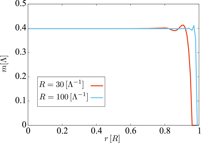
Figure 1: Inhomogeneous dynamical mass as a function of the radial coordinate $r$. Apart from the very vicinity of the boundary $\sim R$, the position dependence is mild enough to justify the local density approximation and Eq. (22). The vanishing mass at the boundary is a consequence from the condition (9). As $R$ increases, the oscillation behavior becomes small, and eventually vanishes.

5 Anomalous coupling to the rotation

So far we have seen that the rotation does not affect the condensate. (Microscopic quantities, e.g., the Dirac eigenvalue can however be affected by rotation, in analogy to the finite density effect.) Nevertheless,the rotation can change the physical properties via anomalous coupling. Here let us pick up two well-known such examples.

The first example is the finite temperature. We know that the rotating fermionic system develops an axial current at finite $T$ [2, 3] as

$$\boldsymbol{j}_{\text{A}}^{\,\text{CVE}}=\frac{T^{2}\boldsymbol{\Omega}}{12}+\frac{\Omega^{2}\boldsymbol{\Omega}}{48\pi^{2}}+O(\Omega R^{-2})\quad\text{for}\ T\gg R^{-1}\geq\Omega\,,$$ (27)

where we drop the finite size corrections of $O(\Omega R^{-2})$. Intuitively we can understand this in the following manner. For sufficiently high $T\gg R^{-1}$, it is unlikely that the bulk constraint at the boundary remains relevant because of the thermal screening and we can safely neglect the boundary effects. Indeed, in this case of $T\gg R^{-1}$, the first term should be much larger than the second one because the causality constraint demands $R^{-1}\geq\Omega$ and thus $T\gg\Omega$. Interestingly, it is known that this coefficient of the term $\propto T^{2}$ is related to the chiral anomaly coming from not gauge fields but Riemann tensors. We can therefore say that the rotation effect becomes visible thanks to the coupling to the gravitational chiral anomaly [22, 23]. (This terminology might be a little confusing; the genuine gravity is irrelevant and what does matter is the chiral anomaly coupled to the Riemann and stress tensors.)

It would be a very interesting question whether the current still persists for $T\lesssim R^{-1}$, and to clarify this, we should do the microscopic calculation with the boundary effects, which was already pointed out in Ref. [3]. Then, the only change from the zero to the finite temperature results is how the effective chemical potential appears, i.e. $\theta\,(\varepsilon-|\Omega j|)$ should be replaced with the Fermi distribution function $[1+e^{-(\varepsilon-|\Omega j|)/T}]^{-1}$, and then we see that $\Omega$ dependence remains even for $\varepsilon>|\Omega j|$. Such an explicit calculation of the chiral vortical effect in a finite size system will be reported elsewhere.

Second, we shall turn to magnetized rotating matter as discussed in Ref. [29]. Under a strong magnetic field, the Landau wave-function is localized and can be even more squeezed than the system size if $\sqrt{eB}\gg R^{-1}$. Then, the boundary effects are essentially irrelevant. Also, the energy dispersion relation of fermions with $B$ is Landau-quantized and the dynamics of the magnetized fermions is dominated by the Landau zero mode, which is independent of the angular momentum. This is quite different from rotating fermions without $B$ for which the IR modes are gapped as seen in Eq. (23). Therefore, there always exist low-energy modes that are Pauli blocked, and thus, with help of finite $B$, the rotation comes to affect the system even at zero temperature. This is an hand-waving explanation for the reason why it has been observed in Ref. [29] that the rotation affects the chiral condensate.

Interestingly, in this case too, the quantum anomaly plays a crucial role. Unlike the temperature for which the gravitational mixed anomaly is relevant, the well-known standard chiral anomaly in terms of the gauge field is sufficient to understand how the rotation and the magnetic field can induce a finite density. To see this explicitly, let us consider a Dirac fermion in the magnetic field $\boldsymbol{B}=B\hat{\boldsymbol{z}}$ without rotation. The Lagrangian density is simply $\mathcal{L}=\bar{\psi}i\gamma^{i}(\partial_{i}+ieA_{i})\psi$, where $A_{i}=(0,By/2,-Bx/2,0)$ in the symmetric gauge choice. Now, we shall perform the “Floquet transformation” [14] or go to the rotating frame by changing,

$$\psi\to\exp(\gamma^{1}\gamma^{2}\Omega t/2)\,\psi\;,$$ (28)

together with the coordinate transformation by $x\to(\cos\Omega t)x-(\sin\Omega t)y$ and $y\to(\cos\Omega t)y+(\sin\Omega t)y$. Then, the Lagrangian density after the transformations reads,

$$\begin{split}\mathcal{L}=\bar{\psi}[i\gamma^{0}\partial_{t}+i\gamma^{1}(\partial_{x}+ieBy/2)&+i\gamma^{2}(\partial_{y}-ieBx/2)\\ &+i\gamma^{3}\partial_{z}+(\Omega/2)\gamma^{3}\gamma_{5}]\psi\,.\end{split}$$ (29)

Here, we can regard the last term proportional to $\Omega/2$ as an axial gauge field or the chiral shift [40], and as calculated in Ref. [13], a finite density is induced from the quantum anomaly coupled with the chiral shift term and the magnetic field as

$$n_{\text{spin}}=\frac{eB\Omega}{4\pi^{2}}\,,$$ (30)

which explains the expression for the density obtained in Ref. [32].

In the above discussions one might have realized that Eq. (29) is not really the Lagrangian density with $B$ in a rotating frame, in which more terms like $\Omega(-x\partial_{y}+y\partial_{x})$ should appear. These terms do not enter Eq. (29) because the Floquet transformation Eq. (28) does not accompany the rotation of the orbital part. In fact we can show that the above anomalous density picks up a contribution from the spin part only.

Because we already know the complete expression for the thermodynamics potential or the free energy with both $B$ and $\Omega$ in Ref. [29], it is easy to take its chemical potential derivative and compute the density. The free energy under strong $B$ enough to discard the boundary effects reads,

$$\begin{split}F&=-\frac{1}{\pi R^{2}}\sum_{q=\pm}\int_{-\infty}^{\infty}\frac{dp_{z}}{2\pi}\sum_{n=0}^{\infty}\alpha_{n}\\ &\qquad\times\sum_{\ell=-n}^{N-n}\biggl{\{}\frac{\varepsilon+q\Omega j+q\mu}{2}+T\ln\bigl{[}1+e^{-(\varepsilon+q\Omega j+q\mu)/T}\bigr{]}\biggr{\}},\end{split}$$ (31)

where $\alpha_{n}=2-\delta_{n,0}$, $j=\ell+1/2$, $N=eBR^{2}/2$, and $\varepsilon=\sqrt{p_{z}^{2}+2neB}$. By differentiating $F$ with respect to $\mu$ and taking the $T\to 0$ limit, the number density in the lowest Landau approximation turns out to be

$$n_{\text{total}}=\frac{\Omega}{\pi^{2}R^{2}}\sum_{\ell=0}^{N}(\ell+1/2)=\frac{eB\Omega}{4\pi^{2}}(N+1)\;.$$ (32)

We see that, in addition to the anomaly-induced density in Eq. (30), we have an extra contribution from the orbital angular momentum $\ell$, which makes a contrast to the result in Ref. [32]. We emphasize that the total angular momentum (i.e., both the orbital and spin angular momentum) contribute this anomalous effect. What we can learn from the above exercises is that the rotation can affect the thermodynamic properties and thus modify the condensate if a strong magnetic field is imposed.

We already mentioned that the intermediate region is difficult to investigate. For the temperature effect, what happens for $T\lesssim R^{-1}$ still needs careful considerations, and in the same way for the magnetic effect, it would be a quantitatively subtle question to study the regime for $\sqrt{eB}\lesssim R^{-1}$. In most of physics problems involving quarks and gluons, either $T\gg R^{-1}$ (in a quark-gluon plasma) or $\sqrt{eB}\gg R^{-1}$ (in a neutron star) would be realized, but for future applications to table-top experiments, a more complete treatment over the whole regime would become important.

References

- [1] A. Vilenkin, Phys. Lett. B80 (1978) 150.
- [2] A. Vilenkin, Phys. Rev. D20 (1979) 1807.
- [3] A. Vilenkin, Phys. Rev. D21 (1980) 2260.
- [4] Z.T. Liang and X.N. Wang, Phys. Rev. Lett. 94 (2005) 102301, nucl-th/0410079, [Erratum: Phys. Rev. Lett.96,039901(2006)].
- [5] X.G. Huang, P. Huovinen and X.N. Wang, Phys. Rev. C84 (2011) 054910, 1108.5649.
- [6] X.G. Huang, Rept. Prog. Phys. 79 (2016) 076302, 1509.04073.
- [7] F. Becattini and F. Piccinini, Ann. Phys. (Amsterdam) 323 (2008) 2452 .
- [8] F. Becattini et al., Ann. Phys. (Amsterdam) 338 (2013) 32 .
- [9] F. Becattini et al., Eur. Phys. J. C75 (2015) 406, 1501.04468.
- [10] Y. Jiang, Z.W. Lin and J. Liao, (2016), 1602.06580.
- [11] A. Aristova et al., (2016), 1606.05882.
- [12] W.T. Deng and X.G. Huang, Phys. Rev. C93 (2016) 064907, 1603.06117.
- [13] S. Ebihara, K. Fukushima and T. Oka, Phys. Rev. B93 (2016) 155107, 1509.03673.
- [14] M. Bukov, L. D’Alessio and A. Polkovnikov, Advances in Physics 64 (2015) 139, 1407.4803.
- [15] N.K. Wilkin and J.M.F. Gunn, Phys. Rev. Lett. 84 (2000) 6.
- [16] A.L. Fetter, Rev. Mod. Phys. 81 (2009) 647.
- [17] K. Mameda and A. Yamamoto, (2015), 1504.05826.
- [18] D.T. Son and A.R. Zhitnitsky, Phys. Rev. D70 (2004) 074018, hep-ph/0405216.
- [19] D.T. Son and P. Surowka, Phys. Rev. Lett. 103 (2009) 191601, 0906.5044.
- [20] D.E. Kharzeev, L.D. McLerran and H.J. Warringa, Nucl. Phys. A803 (2008) 227, 0711.0950.
- [21] K. Fukushima, D.E. Kharzeev and H.J. Warringa, Phys. Rev. D78 (2008) 074033, 0808.3382.
- [22] K. Landsteiner, E. Megias and F. Pena-Benitez, Phys. Rev. Lett. 107 (2011) 021601, 1103.5006.
- [23] G. Basar, D.E. Kharzeev and I. Zahed, Phys. Rev. Lett. 111 (2013) 161601, 1307.2234.
- [24] K. Fukushima and P. Morales, Phys. Rev. Lett. 111 (2013) 051601, 1305.4115.
- [25] K.G. Klimenko, Z. Phys. C54 (1992) 323.
- [26] K.G. Klimenko, Theor. Math. Phys. 90 (1992) 1, [Teor. Mat. Fiz.90,3(1992)].
- [27] V.P. Gusynin, V.A. Miransky and I.A. Shovkovy, Phys. Rev. Lett. 73 (1994) 3499, hep-ph/9405262, [Erratum: Phys. Rev. Lett.76,1005(1996)].
- [28] V.P. Gusynin, V.A. Miransky and I.A. Shovkovy, Nucl. Phys. B462 (1996) 249, hep-ph/9509320.
- [29] H.L. Chen et al., Phys. Rev. D93 (2016) 104052, 1512.08974.
- [30] D. Ebert et al., Phys. Rev. D61 (1999) 025005, hep-ph/9905253.
- [31] F. Preis, A. Rebhan and A. Schmitt, JHEP 03 (2011) 033, 1012.4785.
- [32] K. Hattori and Y. Yin, (2016), 1607.01513.
- [33] Y. Jiang and J. Liao, (2016), 1606.03808.
- [34] P.C.W. Davies, T. Dray and C.A. Manogue, Phys. Rev. D53 (1996) 4382, gr-qc/9601034.
- [35] N. Birrell and P. Davies, Quantum Fields in Curved SpaceCambridge Monographs on Mathematical Physics (Cambridge University Press, 1984).
- [36] V.E. Ambrus and E. Winstanley, Phys. Rev. D93 (2016) 104014, 1512.05239.
- [37] M. Hortacsu, K.D. Rothe and B. Schroer, Nucl. Phys. B171 (1980) 530.
- [38] M. Buballa and S. Carignano, Prog. Part. Nucl. Phys. 81 (2015) 39, 1406.1367.
- [39] C. Giordano and A. Laforgia, Journal of Computational and Applied Mathematics 9 (1983) 221 .
- [40] E.V. Gorbar, V.A. Miransky and I.A. Shovkovy, Phys. Rev. C80 (2009) 032801, 0904.2164.