Episodic Model For Star Formation History and Chemical Abundances in Giant and Dwarf Galaxies

Abstract

In search for a synthetic understanding, a scenario for the evolution of the star formation rate and the chemical abundances in galaxies is proposed, combining gas infall from galactic halos, outflow of gas by supernova explosions, and an oscillatory star formation process. The oscillatory star formation model is a consequence of the modelling of the fractional masses changes of the hot, warm and cold components of the interstellar medium. The observed periods of oscillation vary in the range $(0.1-3.0)\times 10^{7}$ yr depending on various parameters existing from giant to dwarf galaxies. The evolution of metallicity varies in giant and dwarf galaxies and depends on the outflow process. Observed abundances in dwarf galaxies can be reproduced under fast outflow together with slow evaporation of cold gases into hot gas whereas slow outflow and fast evaporation is preferred for giant galaxies. The variation of metallicities in dwarf galaxies supports the fact that low rate of SNII production in dwarf galaxies is responsible for variation in metallicity in dwarf galaxies of similar masses as suggested by various authors.

1 Introduction

The delineation of star formation history (SFH) in galaxies has become an increasingly powerful method for shaping galaxy formation and evolution. For our own Galaxy we can observe that a large number of stars and SFH is directly inferred from the age distribution of stars. For distant galaxies the Hubble Space Telescope is a powerful tool to resolve stellar populations into SFH (Gallert et al. 2005). Star forming galaxies that sample the faint end of galaxy luminosity function are not well studied like brighter, more massive galaxies due to completeness limits of large galaxy surveys (e.g., SDSS). Several authors (Lee et al. 2007; Kennicutt et al. 2008) have found marked differences in H_α equivalent width (EW) measurements, normalized star formation rate (SFR) over the past 5 Myr, for star forming galaxies fainter than $M_{B}\sim-15$ in comparison to brighter galaxies. Different physical mechanisms like stochastic effects (Mueller & Arnett 1976; Gerola & Seiden 1978), internal feedback (stellar winds, supernova; e.g. Pelupessy et al. 2004; Stinson et al. 2007), galaxy interactions (merger, tidal influences; e.g. Toomre & Toomre 1972; Gnedin 1999) have been proposed to shed light in each of such processes. Also there are observational differences in birth rate parameters ($b$), fraction of stars formed per time interval ($f$), spatial distribution of stellar components in dwarf galaxies (Weisz et al. 2008). There are differences in duty cycles (the time for which the SFR is higher than a threshold value) for giants and dwarfs also (Jaacks et al. 2012; Lee et al. 2009) in case of episodic star formation history.

A number of papers have investigated the formation (Burkert et al. 1992; Chattopadhyay et al. 2012; Chattopadhyay et al. 2009; Chattopadhyay & Chattopadhyay 2007) and chemical evolution (Matteucci & Francois 1989; Amarsi et al. 2014; Homma et al. 2015; Zahid 2014; de Boer et al. 2012) of the galaxies and other spiral galaxies (Lynden Bell 1975; Sommer-Larsen 1991). Formation of galactic disc through gas infall from the halo has been suggested also by many authors (Twarog 1980; Hirashita et al. 2001; Narayanan et al. 2015; Aumer et al. 2010; Combes 2008; Haywood et al. 2015). Kennicutt et al. (1994) have suggested that episodic star formation history and the star formation activities differ for early and late type galaxies. Episodic star formation has been suggested by de Boer et al. (2012), Nichols et al. (2012) and many others. All the observational as well as theoretical studies demand an appropriate modelling of the SFH and chemical history of the giant as well as dwarf galaxies taking into consideration most of the physical mechanisms like infall, feedback etc prevailing in these galaxies.

In the present work we give a synthetic model for the episodic star formation in giant as well as in dwarf galaxies through a fast and slowly damping cyclic scenario. For modelling the chemical history we consider infall from halos of galaxies together with outflow of gas due to supernova explosions. We assume that the amount of gas mass driven out by the supernovae in the form of wind is proportional to the instantaneous star formation rate neglecting the time delay of $\lesssim 10^{7}$ years between the star formation and subsequent supernova explosions (Samui 2014). Section 2 describes the mathematical model. In section 3 we discuss about the values of the parameters chosen for our study. Results and discussions are given in sections 4 and 5. Section 6 outlines the main conclusions.

2 Mathematical Model

2.1 Dynamical model of star formation in interstellar medium

The present mathematical model is mainly based on the model suggested by Ikeuchi & Tomita (1983) (hereafter IT83) which was subsequently improved by Hirashita & Kamaya (2000) and Hirashita et al. (2001). According to the above model, star formation in a giant galaxy takes place in the gaseous component consisting of three parts, the hot, warm, and cold gas with fractional masses $X_{\mathrm{h}}$, $X_{\mathrm{w}}$, $X_{\mathrm{c}}$ respectively. The relative abundances of the above mentioned fractional masses are controlled by supernova remnants (SNR) through the following processes, already included in IT83: (i) sweeping of warm gas into cold component ($aX_{\mathrm{w}}$, $a\sim 5\times 10^{-8}$ yr^-1), (ii) evaporation of cold clouds embedded in hot gas ($bX_{\mathrm{c}}X_{\mathrm{h}}^{2}$, $b\sim 10^{-7}-10^{-8}$ yr^-1), (iii) cooling of hot gas in warm gas ($cX_{\mathrm{w}}X_{\mathrm{h}}$, $c\sim 10^{-6}-10^{-7}$ yr^-1). In the present work we have included one more process, which is the sweeping of hot gas into cold gas ($fX_{\mathrm{h}}$). Then the corresponding time rate of change of the fractional masses reduce to,

$$\frac{dX_{\mathrm{c}}}{dt} = aX_{\mathrm{w}}-bX_{\mathrm{c}}X_{\mathrm{h}}^{2}+fX_{\mathrm{h}},$$ (1)

$$\frac{dX_{\mathrm{w}}}{dt} = \!\!\!\!\!-aX_{\mathrm{w}}+cX_{\mathrm{w}}X_{\mathrm{h}},$$ (2)

$$\frac{dX_{\mathrm{h}}}{dt} = bX_{\mathrm{c}}X_{\mathrm{h}}^{2}-cX_{\mathrm{w}}X_{\mathrm{h}}-fX_{\mathrm{h}},$$ (3)

where the coefficients $a$, $b$, $c$, and $f$ are constants.

We normalize the time $t$ and the coefficients as, $\tau=ct$, $A=a/c$, $B=b/c$, $F=f/c$ and normalize the mass fractions by $X_{\mathrm{c}}+X_{\mathrm{h}}+X_{\mathrm{w}}=1$. Then the system of three differential equations reduces to two. Substituting $x=X_{\mathrm{c}}$, and $y=X_{\mathrm{h}}$, we have

$$\frac{dx}{d\tau} = A(1-x-y)-Bxy^{2}+Fy,$$ (4)

$$\frac{dy}{d\tau} = -y(1-x-y)+Bxy^{2}-Fy.$$ (5)

The above set of equations can be treated as a system of coupled polynomial ordinary differential equations including up to third degree terms. The fractional mass condition limits the phase space to the triangular domain $x\geq 0$, $y\geq 0$, $x+y\leq 1$.

We study the phase space structure first through its stationary states, or fixed points, which are derived in detail in the Appendix:

1. $\left\{x=1,y=0\right\}$,

2. $\left\{x=\frac{1-A+F}{1+AB},y=A\right\}$,

3. $\left\{x={1\over 2}-\sqrt{{1\over 4}-F/B},y={1\over 2}+\sqrt{{1\over 4}-F/B}\right\}$,

4. $\left\{x={1\over 2}+\sqrt{{1\over 4}-F/B},y={1\over 2}-\sqrt{{1\over 4}-F/B}\right\}$.

Solution (i) exists for any value of $A$, $B$, and $F$, and does not depend on them. This is an extreme case where all the mass is in the cold phase $X_{\mathrm{c}}=1$.

Solution (ii) depends on all three parameters $A$, $B$, and $F$, and admits values of $X_{\mathrm{c}}$, $X_{\mathrm{w}}$, and $X_{\mathrm{h}}$ in the interval $[0-1]$ for suitable positive $A$, $B$, and $F$, subject to restrictions, such as $F\leq AB(1-A)$, and $0\leq A\leq 1$.

Solutions (iii), and (iv) depend only on $B$, and $F$. Since for each of them $x+y=1$, the warm phase fraction vanishes, $X_{\mathrm{w}}=0$, for any value of $B$, and $F$. To exist these solutions need to be real, which gives a constraint on the parameters, $B\geq 4F$.

In case of giant molecular clouds $X_{\mathrm{c}}$, $X_{\mathrm{h}}$, $X_{\mathrm{w}}$ should be all positive to some extent, the cases where $X_{\mathrm{w}}$ vanishes, or both $X_{\mathrm{w}}$ and $X_{\mathrm{h}}$ vanish may be thought as some kind of exceptional limiting conditions where proper mixing or supernova explosions have not taken place. Therefore solution (ii) is the only stationary point representing a realistic stationary situation for star forming clouds.

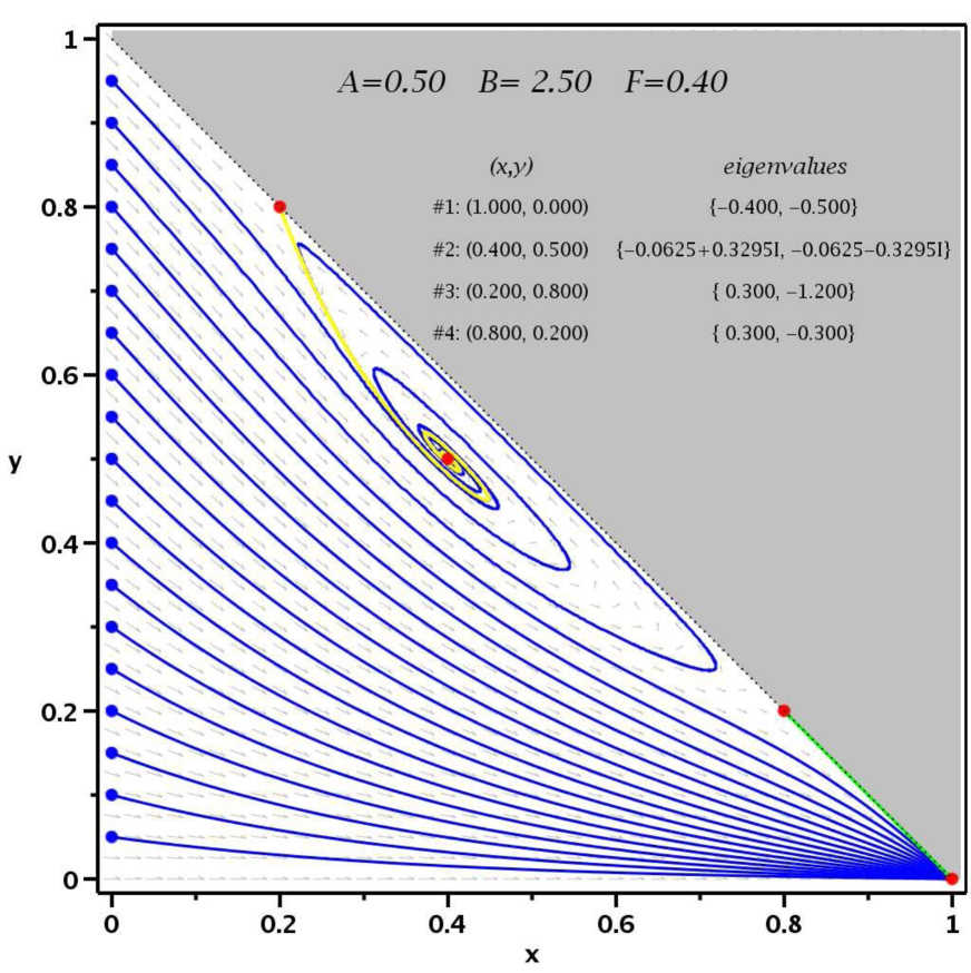
Figure 1: Phase space plot for $A=0.5$, $B=2.5$, $F=0.4$. The velocity field is indicated with grey arrows. The stationary points are marked by red dots, their respective $(x,y)$ coordinates are indicated, as well as their eigenvalues. The blue curves are particular solutions starting at the positions indicated by blue dots. The yellow and green curves are particular solutions starting near unstable stationary point (iii) and (iv). The complex and stable stationary point (ii) attracts nearby phase space with inward spiral motion.

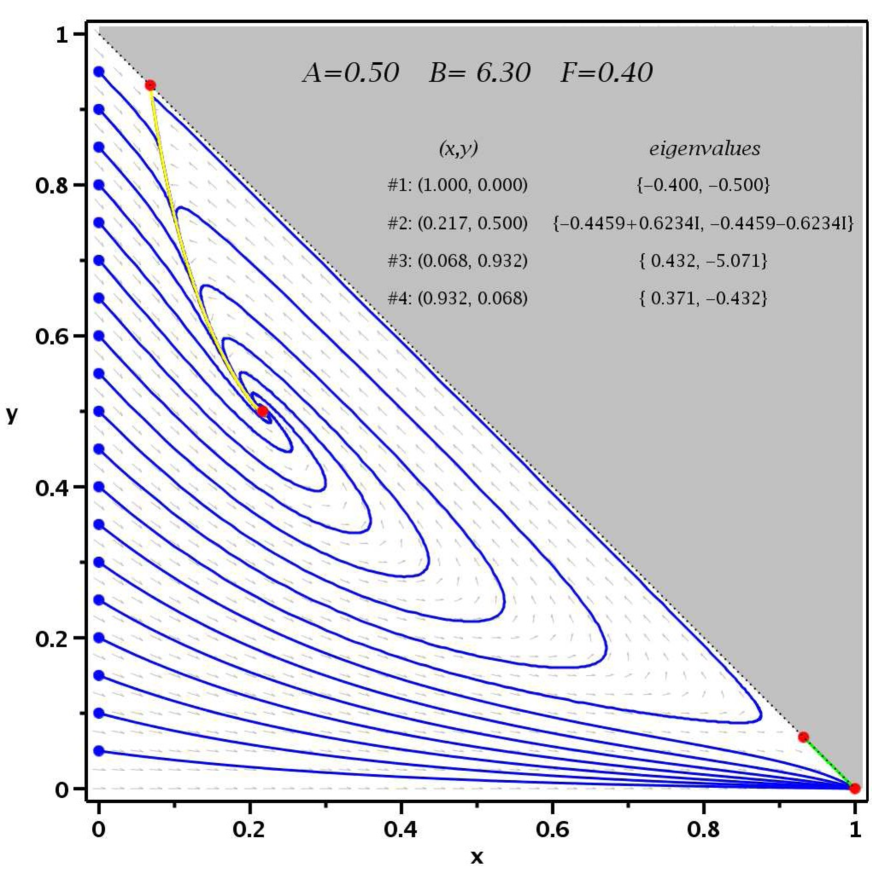
Figure 2: Phase space plot for $A=0.5$, $B=6.3$, $F=0.4$, as in Fig. 1.

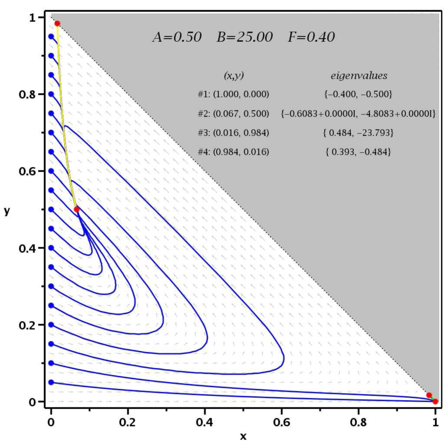
Figure 3: Phase space plot for $A=0.5$, $B=25.$, $F=0.4$, as in Fig. 1, except that stationary point (ii) is here real, so the nearby phase space does not rotate.

Also it follows (Appendix) that for $0<A<1.0$, $0<F<AB(1-A)$ point (ii) moves within the triangle $x\geq 0,y\geq 0$ and $x+y<1$ (Figs. 1–4). The figures indicate that the velocity field may or may not rotate about the stationary point (ii) only. For particular parameters, such as $A=0.4$, $B=2.5$, $F=0.25$ there exists a limit cycle (Fig. 4), which means that the system converges toward a periodic attractor displaying oscillations of its three component abundances and its star formation rate.

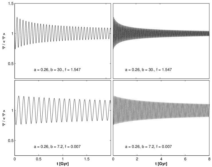
Figure 6: Star formation rate (SFR) for giant (top) and dwarf (bottom) galaxies.

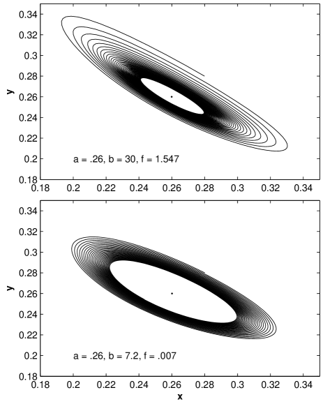
Figure 7: Fast inspiraling behaviour for the stationary point (ii) for higher value of $B$ ($\sim 30$) and slow behaviour for lower value of $B$ ($>2.1$)

Examining the eigenvalues as a function of the parameters ($0<A<1.0$, $0<B<100$, $0\leq F<AB(1-A)$) show that for (ii) (see Fig. 5) the real part is mostly negative and in case of lower values of $B$ the real part is less negative. This means that when $B$ is small, evaporation rate of cold gas to hot gas is less. Lower rate of evaporation means less abundance of hot gas, i.e., lower rate of supernova production. This happens in case of dwarf galaxies. Thus the episodic star formation process prevails for a longer time in dwarf galaxies compared to giant galaxies. For particular parameters, such as $A=0.4$, $B=2.5$ and $F=0.25$ there exists a limit cycle. This means dwarf galaxies are the favourable places for episodic star formation. On the other hand higher values of $B$ is more likely for giant galaxies. Hence episodic star formation process decays rapidly in giant galaxies (viz. Figs. 6, 7). Perhaps this is the reason why giant galaxies do not show evidences of episodic star formation in the last 5 Myr compared to dwarfs (Lee et al. 2007; Kennicutt et al. 2008).

Point (i) is a stable focus (Fig. 8), point (iii) is stable or unstable hyperbolic (Fig. 9) and point (iv) is unstable hyperbolic or stable spiral (Fig. 10). None of these cases provide conditions for episodic star formation.

Thus Figs. 5, 8–10 give a clear demonstration of the existence of cyclic star formation as a function of the various parameters $A$, $B$, $F$. These parameters are representatives of the physical processes occurring in galaxies. Lower values of these parameters correspond to the situation favourable for dwarfs and vice versa as discussed above. In Fig. 5, the real part of $\lambda$ is less negative or zero and the non-zero imaginary part represents an elliptic orbit, which means there exists cycles of slowly decreasing or constant amplitudes for lower values of $A$, $B$, and $F$ whereas rapidly decreasing amplitudes for higher values of $A$, $B$, and $F$. This indicates that around the stationary point (ii) the gas abundances participating in star formation rotates in abundance space either with a slowly decaying manner or continue rotation in case of a limit cycle in dwarfs but always with a rapidly decaying manner in giants. On the other hand for stationary point (i) Fig. 8 shows that $\lambda$ is always negative with no imaginary part, i.e., there exists no cycles for $A$, $B$, and $F$. Figs. 9, 10 indicate that the real part of $\lambda$ has both positive as well as negative values, i.e., the mode of vibration might be stable or unstable. Hence for stationary points other than (ii) there are no cyclic variations in abundance space for any values of the parameters $A$, $B$, and $F$.

2.2 Chemical evolution in galaxies

The chemical evolution in galaxies is based on two phenomena: (i) The gradual gas infall from halos, and (ii) gas outflow as a result of supernova explosion. We have not considered the above two phenomena in the dynamical model of star formation because the infall time scale ($t_{\mathrm{in}}$) is much larger than the oscillatory star formation time scale (viz. average duty cycles, Tables 4, 5). In clusters of galaxies, galaxies move through the intracluster medium and if the ram pressure force exceeds the internal gravitational pull, gas will be stripped from these galaxies (Irwin et al. 1987; White et al. 1991; Böhringer et al. 1995; Balsara et al. 1994). Ram pressure stripping is more efficient in dwarf galaxies compared to giant galaxies due to its low potential well. The time scale of gas removal from dwarf galaxies ($M\lesssim 10^{9}M_{\bigodot}$) is of the order of $2.02\times 10^{8}$ yr and $2.19\times 10^{9}$ yr for massive dwarf galaxies (Mori & Burkert 2001). This is also larger than the oscillatory star formation time scale ($\sim 10^{7}$ yr viz. duty cycles, Tables 4, 5). So the oscillatory model of star formation discussed in section 2.1 does not include the effect of infall as well as outflow.

The changing rates of gas mass ($M_{\mathrm{g}}$) and metal mass ($M_{i}$, $i=$Fe, O, etc.) are mainly based on the work done by Hirashita et al. (2001) but in our case we have included outflow due to supernova explosions. Massive stars would explode as a supernova after $10^{7}$ yr and these explosions drive cold gas out of the galaxy as galactic wind (viz. ram pressure stripping). We assume that the gas mass driven is proportional to the instantaneous star formation rate neglecting the time delay between star formation and subsequent explosion. Then the evolution of gas mass ($M_{\mathrm{g}}$) and metal mass ($M_{\mathrm{i}}$) are governed by the set of differential equations,

$$\frac{dM_{\mathrm{g}}}{dt} = -\psi(t)+R_{\mathrm{ins}}\psi(t)+I(t)-\eta_{\mathrm{w}}\psi(t),$$ (6)

$$\frac{dM_{\mathrm{i}}}{dt}=-X_{i}(t)\psi(t)+\left(R_{\mathrm{ins}}X_{i}(t)+Y_{i,\mathrm{ins}}\right)\psi(t)+I(t)X_{i}^{\mathrm{f}}$$ (7)

where $R_{\mathrm{ins}}$ and $Y_{i,\mathrm{ins}}$ are the instantaneous returned fraction of gas from stars and the fractional mass of the newly formed element $i$ respectively. $X_{i}$ is the abundance of $i$’th element ($X_{i}\equiv M_{i}/M_{\mathrm{g}}$) and $X_{i}^{\mathrm{f}}$ is the abundance of $i$’th element in the infall material (Tinsley 1980). $\eta_{\mathrm{w}}\psi(t)$ is the outflow and $\eta_{\mathrm{w}}$ is a proportionality constant defined as (Samui 2014)

$$\eta_{\mathrm{w}}=\left(\frac{v_{\mathrm{c}}}{v_{\mathrm{c}}^{0}}\right)^{-\alpha}$$ (8)

where $v_{\mathrm{c}}$ is the rotational velocity of the galaxy and $v_{\mathrm{c}}^{0}$ is that when $\eta_{\mathrm{w}}=1$. $\alpha=2$ or 1 on whether the outflows are energy driven or momentum driven. It is clear that for a given $\psi(t)$, outflow is higher for a dwarf galaxy than for a giant galaxy. $I(t)$ is the rate of gas infall from halo at time $t$ and is given by (Hirashita et al. 2001)

$$I(t)=\frac{M_{0}}{t_{\mathrm{in}}}\exp(-t/t_{\mathrm{in}})$$ (9)

where $M_{0}$ is the total mass of infall, $t_{\mathrm{in}}$ is the total time of infall. $\psi(t)$ is the star formation rate at time $t$ and is given by (Hirashita et al. 2001),

$$\psi(t)=M_{\mathrm{g}}x/t_{*}$$ (10)

Dividing Eqs. (6) and (7) by $M_{0}$ and substituting $f_{\mathrm{g}}=\frac{M_{\mathrm{g}}}{M_{0}}$, $\widetilde{\psi}=\frac{\psi}{M_{0}}$ as done by Hirashita et al. (2001) we have

$$\frac{df_{\mathrm{g}}}{dt} = -(1-R_{\mathrm{ins}})\widetilde{\psi}(t)+\frac{1}{t_{\mathrm{in}}}\exp(-t/t_{\mathrm{in}})$$ (11)

$$\qquad\qquad\qquad\qquad-\left(\frac{v_{\mathrm{c}}}{v_{\mathrm{c}}^{0}}\right)^{-\alpha}\widetilde{\psi}(t),$$

$$\ f_{\mathrm{g}}\frac{dX_{i}}{dt} = Y_{i,\mathrm{ins}}\widetilde{\psi}(t)-\frac{X_{i}(t)-X_{i}^{\mathrm{f}}}{t_{\mathrm{in}}}\exp(-t/t_{\mathrm{in}})$$ (12)

$$\qquad\qquad\qquad\qquad+X_{i}(t)\left(\frac{v_{\mathrm{c}}}{v_{\mathrm{c}}^{0}}\right)^{-\alpha}\widetilde{\psi}(t)$$

3 Initial values of the parameters

We have chosen the values of the parameters $Y_{i,\mathrm{ins}}$, $X_{i}^{\mathrm{f}}$, $R_{\mathrm{ins}}$, $t_{*}$, $t_{\mathrm{in}}$ from Hirashita et al. (2001). We have chosen the values of $A$, $B$ and $F$ as discussed in section 2.1. Samui (2014) has discussed on $v_{\mathrm{c}},v_{\mathrm{c}}^{0}$ and $\alpha$. For dwarf galaxies $v_{\mathrm{c}}$ varies from $10\rm\,kms^{-1}$ to $30\rm\,kms^{-1}$ whereas for giants the range is from $100\rm\,kms^{-1}$ to $800\rm\,kms^{-1}$. The parameter $\alpha$ varies from 1 to 2. Hence we have chosen the parameters accordingly so that they can produce observed metallicities for giant as well as dwarf galaxies. All the values of the parameters considered are given in Table 2.

4 Results

In the present work we have tried to model an episodic star formation history and metal production observed in giant as well as in dwarf galaxies. For the dynamical model we have included an additional mechanism of sweeping of hot gas into cold gas besides sweeping of warm gas into cold gas to represent a more realistic situation of giant molecular clouds. Also in the model of metal evolution we have added outflow of gas from galaxies due to supernova explosions. This helps to study the evolution of metallicity in giant as well as in dwarf galaxies under various parametric conditions. While studying the star formation rate (SFR) we have found a stationary point (ii) around which a slow elliptic inspiraling behaviour of the eigenvalue exists for lower values of $B$ (Figs. 1, 2, 3, 5) whereas the process is fast for higher values of $B$ (e.g., $B=25$ in Fig. 3). Under special parameter condition there exists a limit cycle (Fig. 4 and Appendix), e.g., $A=0.4$, $B=2.5$, $F=0.25$. Tables 1, 3 show the average star formation rates and abundances in giants and dwarf galaxies for various values of $A$, $B$ and $F$. It is clear that both $B$ and $F$ are lower and higher in dwarfs and giants respectively to produce observed abundances whereas values of $A$ are similar for both kind. The average star formation rate is higher in giants than in dwarfs. The above trend suggests that in dwarfs due to lower rate of supernova production, mixing of hot gas and evaporation of cold gas is lower but due to less amount of gas the SFR is lower compared to giants where in spite of larger evaporation ($B$ is higher) and fast mixing ($F$ is larger) the SFR is higher due to higher potential well. The variation of metal abundances in dwarfs of similar masses supports the results derived by Kroupa (2004) that low rate of SNII production in dwarf galaxies is responsible for the variation of metallicities in dwarfs of similar masses. This leads to the fact that galaxian stellar initial mass function is very much influenced by the galaxy masses which in turn affects the star formation history. Cosmologically this implies that the number of SNII per low-mass star is significantly depressed and that chemical enrichment process is much slower in dwarf galaxies with a low average star-formation rate compared to giant galaxies.

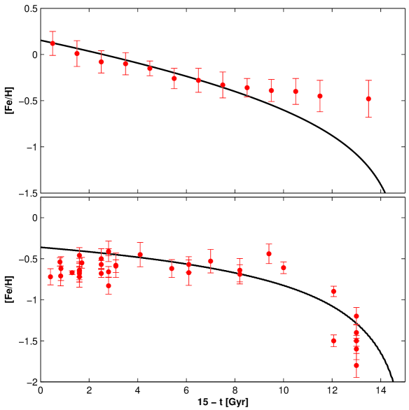
Figure 11: Age-metallicity ([Fe/H]) diagram for giant (top) and dwarf (bottom) galaxies for particular values of the input parameters. The red dots are observations from Rocha-Pinto et al. (2000) (top) and Chattopadhyay et al. (2012) (bottom).

In Fig. 11 we have compared the predicted iron abundances at different times for giant and dwarf galaxies with the observed ones from Rocha-Pinto et al. (2000) and Chattopadhyay et al. (2012). The age-metallicity evolution gives good fit both for giant as well as dwarf galaxies ($p$-values are 0.713 and 0.653 excluding few outliers, for giants and dwarfs respectively). Tables 4 and 5 list the ratio of average star formation rates in the last 100 Myr, 500 Myr, 1 Gyr normalized to the life time average star formation rate (viz. $b_{100},b_{500},b_{1000}$) and average duty cycles for giant and dwarf galaxies for various initial values of the parameters (viz. $A$, $B$, $F$) and they are compared with the corresponding observed quantities for dwarf irregular galaxies of M81 group (Weisz et al. 2008). The values for dwarf galaxies are very close to the observed ones in most cases. The differences might be due to the fact that Weisz et al. (2008) considered only a particular type of dwarf galaxies e.g. dwarf irregulars (dIrr) other than considering all species e.g. dwarf ellipticals (dE) or dwarf spheroidals (dSph) under different abundance properties. The average duty cycles for giant and dwarf galaxies are in the ranges $(0.1-3.2)\cdot 10^{7}$ yr and $(0.1-0.6)\cdot 10^{7}$ yr respectively. The duty cycles for giants are initially larger and rapidly die out whereas those for dwarfs remain more or less similar.

5 Discussion

Eigenvalues plots as a function of the parameters shows that out of the four stationary points (ii) is the only possible stable stationary state for a three-phase medium which is stable for particular values of the parameters. For (ii) the real part of complex eigenvalues when negative indicates that the stationary point is stable, and the non-zero imaginary part indicates that nearby solutions rotate around the point. When the real part of eigenvalue is less negative, i.e., $B$ is small, the decay is slow and when real part of eigenvalue is more negative, i.e., $B$ is larger, the orbit decays faster. There exists a stable attractor only under very special parametric situations, e.g., $A=0.4$, $B=2.5$, $F=0.25$ where star formation remains episodic over the entire period. We have already mentioned that smaller values of $B$ are likely in dwarf galaxies and vice versa. Also limit cycle behaviour exists for small $B$. Hence episodic star formation has frequent occurrence in dwarf galaxies for all the time and for the initial phases only in giant galaxies. Thus in giant galaxies other processes of star formation is preferred (e.g., galaxy interaction etc.) over episodic process.

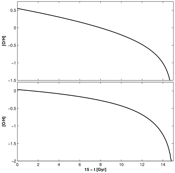
Figure 12: Age-metallicity ([O/H]) diagram for giant (top) and dwarf (bottom) galaxies for particular values of the input parameters.

The model and results indicate that the observed metal abundances for giants and dwarfs are reproduced for larger and smaller values of $B$ respectively. From Tables 1, 3 we find that in dwarf galaxies, due to low potential well, the amount of gas available for star formation is much less compared to giant galaxies. Hence rate of supernova production is less in dwarfs compared to giants. As a result evaporation rate of cold gas into hot gas is low. Since SFR is proportional to the amount of cold gas, average SFR is lower in (viz. Table 1, column 4) these dwarfs due to low potential well than in giant galaxies (viz. Table 3, column 4), where $B$ is higher. Hence enough cold gas is available for star formation in spite of higher evaporation rate due to higher potential well resulting in a higher average star formation rates. Since rate of supernova explosions is lower in dwarfs compared to that of giants, heavy metals are less abundant in dwarfs rather than giants (viz. Tables 1, 3, Figs. 11, 12). In our model outflow has been considered, to be originated due to driven out of hot gas as a result of supernova explosions. In such outflow it is inversely proportional to the square of the circular velocity of the galaxy (Samui et al. 2010). Now the circular velocity of dwarf galaxies vary from $10\rm\,km\,s^{-1}$ to $30\rm\,km\,s^{-1}$, which is very low compared to that of giant galaxies. Hence in dwarf galaxies the rate of outflow is much higher than that of giant galaxies. This also reduces the process of star formation and as a result the metal production is lower in dwarfs than in giants. The birth rate of stars in the last 100 yr, 500 yr, 1000 yr are more or less the same in dwarfs but vary for giants. Hence it is expected that the starbursts are more likely to happen in the initial phase of star formation history in giant galaxies whereas the birth rates remain the same for dwarfs over the entire star formation history.

6 Conclusion

In the present work an episodic star formation scenario has been proposed for the observed star formation history in giant as well as dwarf galaxies. The model is based on the transition of hot and warm gases into cold gas and vice versa. The rate of transition processes have been treated as parameters to study the behaviours of observable quantities, e.g., duty cycles, birth rates of star formations in the last couple of years, present metallicities in giant as well as dwarf galaxies, and compared with observations. The present model is an extension of the work by Hirashita et al. (2001) taking into additional consideration of (i) sweeping of hot gas into cold gas and (ii) outflow of gas due to supernovae explosion which in turn give a picture of episodic star formation scenario in giant as well as dwarf galaxies. It is found that life time average SFR of dwarfs are lower compared to giant galaxies and the birth rate of stars in the last 100 yr, 500 yr, 1000 yr are more or less the same in dwarfs but vary for giants. Hence it is expected that starbursts are more likely to happen in the initial phase of star formation history in giant galaxies whereas the birth rates remain same for dwarfs over the entire star formation history. The average star formation cycles of dwarfs are smaller than giants by a factor of almost 2 (viz. last columns of Tables 4 and 5). The observed metallicities are produced for a slow sweeping, slow evaporation, and fast outflow of warm and hot gases in dwarfs compared to fast sweeping, fast evaporation, and slow outflow in giants which is compatible with the physical structure of low and high galaxy potential of these respective galaxy types. The variance of metallicities in dwarfs might be due to low rate of SNII production as suggested by many authors.

Appendix A Calculation and stability of the stationary points

Stationary points:

Setting the rhs of Eqs. (4) and (5) to zero we get,

$$A(1-x-y)-Bxy^{2}+Fy = 0,$$ (13)

$$-y(1-x-y)+Bxy^{2}-Fy = 0.$$ (14)

Factoring (14), we obtain two possible constraints for $y$,

$$y=0,$$ (15)

or

$$y=\frac{1+F-x}{1+Bx}.$$ (16)

Substituting the first possibility $y=0$ in Eq. (13) we obtain $x=1$. Hence

$$(x=1,y=0)$$ (17)

is a possible stationary point (viz. (i)). This solution exists for any values of $A$, $B$, and $F$.

Substituting the second possibility Eq. (16) in Eq. (13), we obtain a cubic equation for $x$, which factors as a product of a linear and quadratic terms,

$$\left[(1+AB)x+A-F-1\right]\left[Bx(x-1)+F\right]=0.$$ (18)

Assuming the first term in brackets as zero, we obtain the stationary point (ii),

$$\left(x={1-A+F\over 1+AB},y=A\right),$$ (19)

which depends on $A$, $B$, and $F$. Since physical solutions require $0\leq x,y\leq 1$, $0\leq x+y\leq 1$, $A\geq 0$, $B\geq 0$, and $F\geq 0$, for this stationary point to exist the parameters must additionaly satisfy $0\leq A\leq 1$, and $F\leq AB(1-A)$.

Assuming the second term in brackets in Eq. (18) as zero, and $B>0$, yields two more stationary points, (iii) and (iv),

$$\left(x={1\over 2}\left(1\mp\sqrt{1-{4F\over B}}\right),y={1\over 2}\left(1\pm\sqrt{1-{4F\over B}}\right)\ \right),$$ (20)

which are real and distinct if $0<4F\leq B$. These points do not depend on $A$ and lie on the diagonal $x+y=1$, which implies that the third warm component vanishes, $X_{\mathrm{w}}=0$.

Stability of the stationary points:

The Jacobian matrix $J$ of the dynamical system Eqs. (4) and (5) is,

$$J=\left(\begin{array}[]{cc}-By^{2}-A&-2Bxy-A+F\\ By^{2}+1&2Bxy+x+2y-F-1\end{array}\right).$$ (21)

Hence, $|J-\lambda I|=0$ gives the characteristic polynomial,

$$\lambda^{2}-P\lambda-Q=0,$$ (22)

where,

$$P=-By^{2}+2(Bx+1)y-A-F+x-1,\\$$ (23)

$$Q=2By^{3}-B(A+x+1)y^{2}+(2ABx+A+F)y+A(x-F-1),$$ (24)

For stability, the real part of the eigenvalues must be negative or zero. The eigenvalue of imaginary part indicates that nearby solutions rotate around the stationary point in phase space.

Point (i)

For stationary point (i) the eigenvalues are the solutions for $\lambda$ of Eq. (22), found to be,

$$\lambda_{1}=-A,\quad\lambda_{2}=-F.$$ (25)

Since physically $A,F>0$, this point is always attractive and stable.

Point (ii)

For stationary point (ii), the eigenvalues are more complicated to characterize. Substituting Eq. (19) in Eqs. (23), (24), $P$ and $Q$ for point (ii) read

$$P=\frac{1+F-A^{2}B-2A}{1+1/AB},\quad Q=A(A^{2}B-AB+F).$$ (26)

The discriminant $\Delta=P^{2}+4Q$ of Eq. (22) reads,

$$\Delta={AS\over(AB+1)^{2}},$$ (27)

where $S$ is a quadratic polynomial in $F$,

$$S=c_{2}F^{2}+c_{1}F+c_{0},$$ (28)

where

$$c_{2} = AB^{2},$$ (29)

$$c_{1} = -2A^{3}B^{3}+2AB^{2}+8AB+4,$$ (30)

$$c_{0} = AB(A^{4}B^{3}+8A^{3}B^{2}-6A^{2}B^{2}+$$ (31)

$$\qquad 12A^{2}B-12AB+4A+B-4)$$

The sign of $S$ is also the sign of $\Delta$, which tells whether the eigenvalues are complex or real. Solving Eq. (28) for $F$ knowing $A$ and $B$ gives the limits in the $(A,B,F)$ space for real or complex eigenvalues. The exact boundary in parameter space can be specified by solving multivariate high order polynomials in $A$, $B$, and $F$ for the real and imaginary parts of the eigenvalues. These expressions are too large to show here.

But when the eigenvalues are complex, the sign of $P$ is also the sign of the real part of both eigenvalues, which is also the sign of $1+F-A^{2}B-2A$. Thus $B<(1+F-2A)/A^{2}$, or alternatively $F>A^{2}B+2A-1$ when (ii) is unstable and complex. As seen above, $F<AB(1-A)$ for $(x,y)$ to be real, thus $A^{2}B+2A-1<F<AB-A^{2}B$, or $2A(AB+1)<AB+1$. Since $A$ and $B$ are positive, the additional constraint $A<1/2$ follows.

Fig. 5 shows the real and imaginary part of the eigenvalues for (ii) for $0<A<1.0$, $B=3$, $0<F<1.5$. The real parts are slightly positive when $A<0.5$, $F<0.6$, while the imaginary part is non-zero, which is a necessary but not sufficient condition for the existence of a limit cycle in the neighbourhood of the stationary point.

Points (iii) and (iv)

For stationary points (iii) and (iv), the eigenvalues are

$$\lambda_{1\pm} = -A+{1\over 2}\left(1\pm\sqrt{1-{4F\over B}}\right),$$ (32)

$$\lambda_{2\pm} = 2F-{B\over 2}\left(1\pm\sqrt{1-{4F\over B}}\right).$$ (33)

Since $B\geq 4F$ for the stationary points to exist, these eigenvalues are real, and can be negative or positive. Interestingly, although the positions of the stationary points are indepedent on $A$, the first eigenvalue does depend on $A$.

Figs. 8, 9, and 10 show that points (i), (iii), and (iv) are all stable or unstable, where the nearby orbits are hyperbolic, which means that nearby orbits do not rotate around the points in phase space. This is expected since these stationary points are on the boundary of the triangular physical domain, so nearby real solutions cannot rotate around the stationary point.

Numerical solutions

Over 1600 phase space plots and movies have been numerically computed for $0<A\leq 1$, $0<B\leq 100$, and $0\leq F<AB(1-A)$ for the cases where the stationary point (ii) is inside the physical triangle $0\leq x\leq 1$, $0\leq y\leq 1$ and $x+y\leq 1$. Each plot contains the vector field (in gray) and solutions starting from $x=0$, $y=0.05,0.10,\ldots,0.95$ (in blue), and other solutions starting very close to the four stationary points (in red), which are visible only when the stationary points are unstable. Each solution is integrated up to a time value of 500. In each plot the parameters $A$, $B$, and $F$ are indicated, as well as the positions $(x,y)$ of the four stationary points (i)–(iv), and their respective real or complex eigenvalues.

These particular solutions can be used to check the existence of a stable limit cycle (a periodic oscillating solution) around point (ii). A necessary but not sufficient condition for the existence of such a stable periodic solution is that the point (ii) eigenvalues are complex with positive real part. Further, solutions starting close to some other unstable stationary points must asymptotically wind up around point (ii) keeping a finite distance to it (see Fig. 4), which is granted when point (ii) eigenvalues are complex with positive real part.

When point (ii) eigenvalues are complex but with negative real part all the solutions in its neighbourhood spiral toward point (ii).

The movies are sequences of phase space plots over the parameters missing in the file name, varying $F$ first, $B$ second and $A$ last in ascending order of the parameter values.

The found limit cycles are all consistant with the necessary parameter constraints $A<1/2$, $B<(1+F-2A)/A^{2}$, and $F>A^{2}B+2A-1$ discussed above. For $F=0$ the values of $A$ and $B$ are consistent with that of Hirashita et al. (2001) for the stationary point (ii).

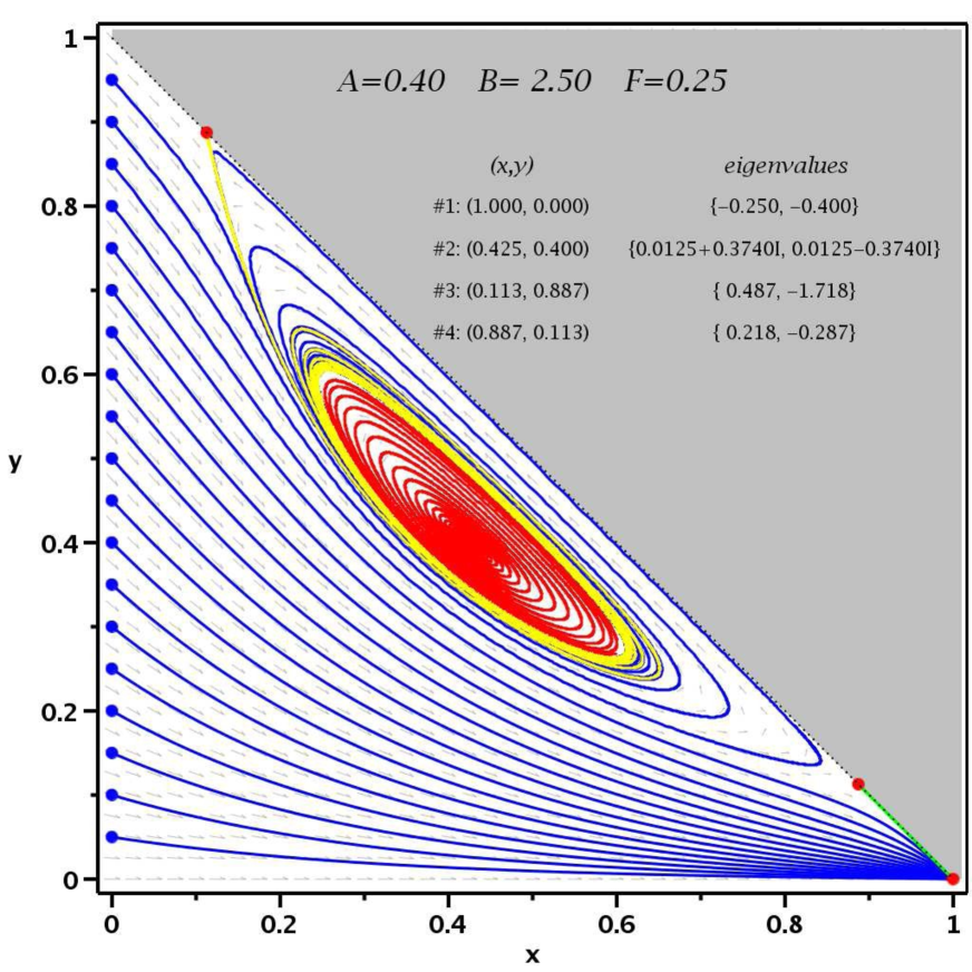
Figure 4: Phase space plot for $A=0.4$, $B=2.5$, $F=0.25$, as in Fig. 1, except that stationary point (ii) is complex, but unstable. The red curve is a particular solution starting near point (ii) and spiraling outward, while the yellow curve spiral inward. Both curves converge toward a stable limit cycle.

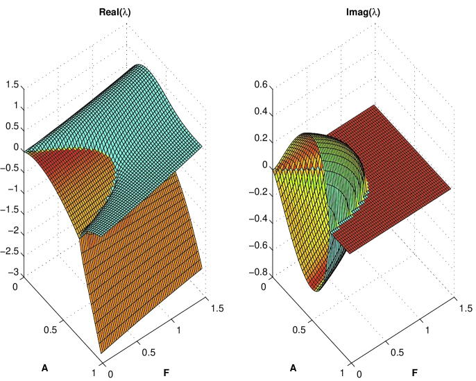
Figure 5: Real (left) and imaginary (right) parts of eigenvalues for the stationary point (ii) for $0\leq A\leq 1.0$, $B=3.0$, $0\leq F\leq 1.5$.

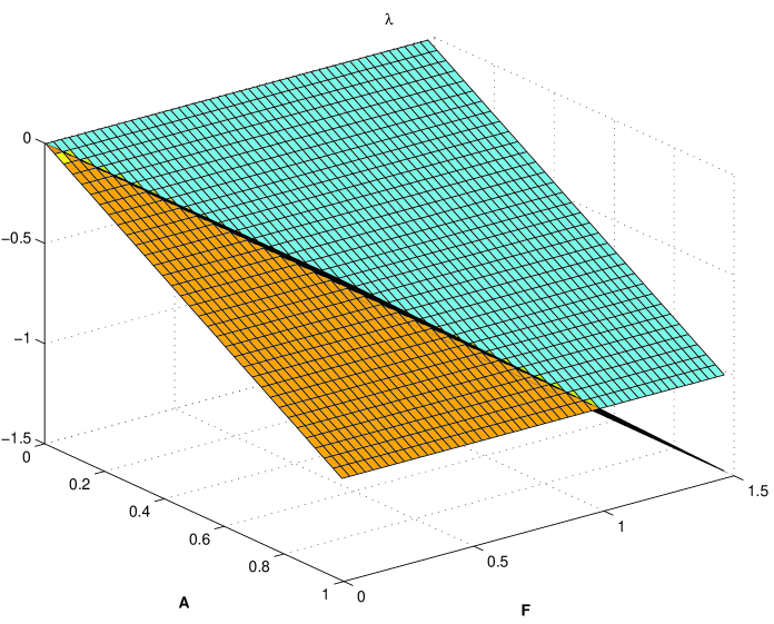
Figure 8: Real parts of eigenvalues for the stationary point (i) for $0\leq A\leq 1.0$, $B=3.0$, $0\leq F\leq 1.5$.

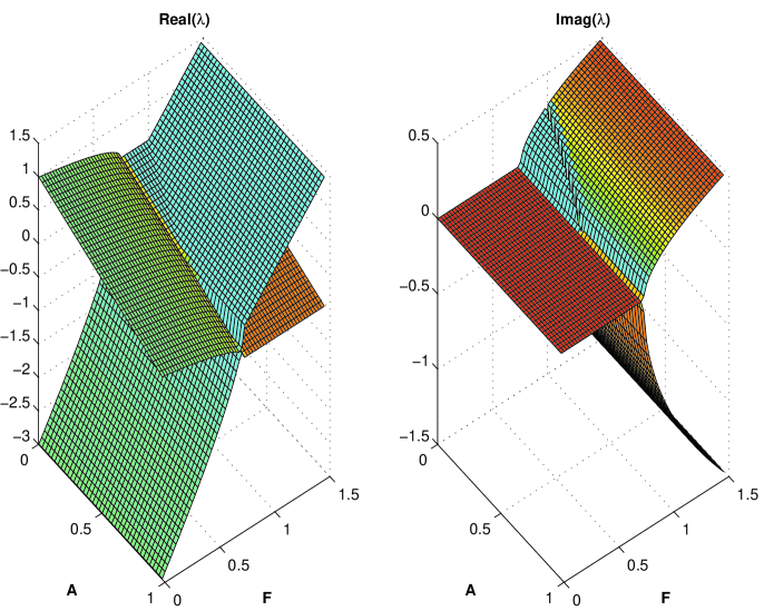
Figure 9: Real (left) and imaginary (right) parts of eigenvalues for the stationary point (iii) for $0\leq A\leq 1.0$, $B=3.0$, $0\leq F\leq 1.5$.

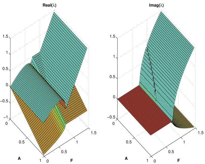
Figure 10: Real (left) and imaginary (right) parts of eigenvalues for the stationary point (iv) for $0\leq A\leq 1.0$, $B=3.0$, $0\leq F\leq 1.5$.

Table 1: Mean SFR and abundances (at 15 Gyr) in dwarf galaxies for various values of input parameters with $t_{*}=2.0\,$Gyr, $t_{\mathrm{in}}=12.0\,$Gyr, $\frac{X_{0}^{\mathrm{f}}}{X_{0,\odot}}=\frac{X_{\mathrm{Fe}}^{\mathrm{f}}}{X_{\mathrm{Fe},\odot}}=0.0$, $R_{\mathrm{ins}}=0.16$, $Y_{0,\mathrm{ins}}/X_{0,\odot}=0.70$, $Y_{\mathrm{Fe},\mathrm{ins}}/X_{\mathrm{Fe},\odot}=0.28$, $v_{\mathrm{c}}=20\rm km\,s^{-1}$, $v_{c0}=100\rm km\,s^{-1}$, $\alpha=1.2$

$A$	$B$	$F$	$\langle\frac{\psi t_{*}}{M_{\mathrm{g}}}\rangle$	$\langle\frac{\psi t_{*}}{M_{\mathrm{g}}}\rangle_{\sigma}$	$\mathrm{[O/H]}_{\mathrm{max}}$	$\mathrm{[Fe/H]}_{\mathrm{max}}$
0.260	7.50	0.016	0.2564	0.00013028	0.0350	-0.3630
0.260	7.51	0.019	0.2572	0.00015528	0.0354	-0.3625
0.260	7.52	0.022	0.2581	0.00019248	0.0358	-0.3621
0.265	7.50	0.016	0.2514	0.00004227	0.0323	-0.3656
0.265	7.51	0.019	0.2522	0.00004468	0.0328	-0.3652
0.265	7.52	0.022	0.2529	0.00004736	0.0332	-0.3647
0.270	7.50	0.016	0.2466	0.00002454	0.0295	-0.3684
0.270	7.51	0.019	0.2474	0.00002538	0.0300	-0.3679
0.270	7.52	0.022	0.2481	0.00002627	0.0305	-0.3675
0.305	7.50	0.016	0.2162	0.00000516	0.0077	-0.3902
0.305	7.51	0.019	0.2169	0.00000521	0.0083	-0.3896
0.305	7.52	0.022	0.2176	0.00000526	0.0089	-0.3890

Table 2: Values of the parameters and initial values of the abundances.

Parameter	values
$A$	$0-1.0$
$B$	$0-100$
$Y_{0,\mathrm{ins}}$ (in $X_{0\odot}$)	0.70
$Y_{\mathrm{Fe},\mathrm{ins}}$ (in $X_{\mathrm{Fe}\odot}$)	0.28
$X_{0}^{\mathrm{f}}$ (in $X_{\mathrm{Fe}\odot})$	0.0
$X_{Fe}^{\mathrm{f}}$ (in $X_{\mathrm{Fe}\odot})$	0.0
$R_{\mathrm{ins}}$	0.16
$t_{*}$ (in Gyr)	1.0, 2.0
$t_{\mathrm{in}}$ (in Gyr)	2.0, 12.0
$v_{\mathrm{c}}$ (in $\rm km\,s^{-1}$)	200, 20
$v_{c0}$ (in $\rm km\,s^{-1}$)	100
$\alpha$	1.2

Table 3: Mean SFR and abundances (at 15 Gyr) in giant galaxies for various values of input parameters with $t_{*}=1.0\,$Gyr, $t_{\mathrm{in}}=2.0\,$Gyr, $\frac{X_{0}^{\mathrm{f}}}{X_{0,\odot}}=\frac{X_{\mathrm{Fe}}^{\mathrm{f}}}{X_{\mathrm{Fe},\odot}}=0.0$, $R_{\mathrm{ins}}=0.16$, $Y_{0,\mathrm{ins}}/X_{0,\odot}=0.70$, $Y_{\mathrm{Fe},\mathrm{ins}}/X_{\mathrm{Fe},\odot}=0.28$, $v_{\mathrm{c}}=200\,\rm km\,s^{-1}$, $v_{c0}=100\,\rm km\,s^{-1}$, $\alpha=1.2$

$A$	$B$	$F$	$\langle\frac{\psi t_{*}}{M_{\mathrm{g}}}\rangle$	$\langle\frac{\psi t_{*}}{M_{\mathrm{g}}}\rangle_{\sigma}$	$\mathrm{[O/H]}_{\mathrm{max}}$	$\mathrm{[Fe/H]}_{\mathrm{max}}$
0.260	30.1	1.55	0.25969	0.00010330	0.55039	0.15245
0.260	30.2	1.56	0.26018	0.00014741	0.55128	0.15334
0.260	30.3	1.57	0.26085	0.00025096	0.55262	0.15468
0.265	30.1	1.64	0.26483	0.00011325	0.56037	0.16243
0.265	30.2	1.65	0.26531	0.00016407	0.56123	0.16329
0.265	30.3	1.66	0.26594	0.00027099	0.56245	0.16451
0.270	30.1	1.73	0.26977	0.00010806	0.56969	0.17175
0.270	30.2	1.74	0.27017	0.00014613	0.57038	0.17244
0.270	30.3	1.75	0.27069	0.00022566	0.57133	0.17339
0.275	30.1	1.82	0.27451	0.00009238	0.57843	0.18049
0.275	30.2	1.83	0.27483	0.00011220	0.57895	0.18101
0.275	30.3	1.84	0.27519	0.00014867	0.57955	0.18161

Table 4: Birth rates in the last 100, 500, 1000 Myr and average duty cycles for giant galaxies for various values of input parameters.

$A$	$B$	$F$	$\langle\frac{\psi t_{*}}{M_{\mathrm{g}}}\rangle$	$b_{100}$	$b_{500}$	$b_{1000}$	average cycle
							(in $10^{7}$yr)
0.260	30.1	1.55	0.26041	0.99957	0.99910	0.99918	0.84750
0.260	30.2	1.56	0.26099	1.00020	0.99844	0.99898	1.99867
0.260	30.3	1.57	0.26160	1.00791	1.00043	0.99962	2.98560
0.265	30.1	1.64	0.26564	0.99979	0.99930	0.99907	1.13534
0.265	30.2	1.65	0.26620	1.00239	0.99973	0.99889	2.21000
0.265	30.3	1.66	0.26680	0.99424	0.99977	0.99844	3.27832
0.270	30.1	1.73	0.27046	0.99875	0.99915	0.99913	0.92132
0.270	30.2	1.74	0.27094	0.99894	0.99933	0.99885	2.10058
0.270	30.3	1.75	0.27145	0.99408	0.99883	0.99880	2.94427
0.275	30.1	1.82	0.27516	0.99916	0.99926	0.99932	0.45329
0.275	30.2	1.83	0.27557	0.99847	0.99903	0.99916	1.11802
0.275	30.3	1.84	0.27599	0.99812	0.99905	0.99904	2.04222
0.280	30.1	1.91	0.27964	0.99952	0.99950	0.99950	0.23935
0.280	30.2	1.92	0.27996	0.99937	0.99939	0.99940	0.35090
0.280	30.3	1.93	0.28030	0.99903	0.99923	0.99930	0.55776
0.305	30.1	2.36	0.30009	0.99999	0.99999	0.99999	0.11861
0.305	30.2	2.37	0.30018	0.99999	0.99999	0.99999	0.12270
0.305	30.3	2.38	0.30026	0.99999	0.99999	0.99999	0.11878

Table 5: Birth rates in the last 100, 500, 1000 Myr and average duty cycles for dwarf galaxies for various values of input parameters and compared with the observed birth rates of dwarf irregular galaxies (Weisz et al. 2008).

$A$	$B$	$F$	$b_{100}$	$b_{100}$	$b_{500}$	$b_{500}$	$b_{1000}$	$b_{1000}$	average cycles.
			(predicted)	(observed, Galaxy name)	(predicted)	(observed)	(predicted)	(observed)	(in $10^{7}$ yr)
0.260	7.50	0.016	0.99951	0.37 (Garland)	0.99951	0.25	0.99950	0.15	0.44958
0.260	7.51	0.019	0.99939	1.84 (Dwarf A)	0.99941	1.08	0.99939	0.92	0.68348
0.260	7.52	0.022	0.99924	1.24 (DDO 53)	0.99932	0.76	0.99931	1.08	1.48730
0.265	7.50	0.016	1.00002	1.38 (IC 2574)	1.00002	1.38	1.00002	1.97	0.14765
0.265	7.51	0.019	1.00000	1.73 ( WLM )	1.00000	2.08	1.00000	2.24	0.13765
0.265	7.52	0.022	0.99999	1.61 (IC 1613)	0.99999	0.95	0.99999	0.83	0.13234
0.270	7.50	0.016	1.00012	1.36 (NGC 3109)	1.00012	1.05	1.00012	0.75	0.11794
0.270	7.51	0.019	1.00012	0.34 (IC 10)	1.00012	1.05	1.00012	0.81	0.11612
0.270	7.52	0.022	1.00011	–	1.00011	–	1.00011	–	0.11638

Table 6: Some parameter values where a limit cycle is found.

$A$	$B$	$F$
0.10	63.00	0.00
0.10	100.00	0.25
0.10	100.00	0.40
0.15	16.00	0.00
0.15	25.00	0.00
0.15	25.00	0.10
0.15	40.00	0.25
0.15	40.00	0.40
0.15	100.00	1.60
0.20	6.30	0.00
0.20	10.00	0.00
0.20	10.00	0.10
0.20	16.00	0.10
0.20	16.00	0.16
0.20	16.00	0.25
0.25	2.50	0.00
0.25	4.00	0.00
0.25	6.30	0.00
0.25	6.30	0.10
0.25	6.30	0.16
0.25	10.00	0.16
0.25	10.00	0.25
0.25	16.00	0.63
0.30	1.00	0.00
0.30	1.60	0.00
0.30	2.50	0.00
0.30	2.50	0.10
0.30	4.00	0.00
0.30	4.00	0.10
0.30	4.00	0.16

$A$	$B$	$F$
0.30	5.00	0.10
0.30	6.30	0.25
0.30	10.00	0.63
0.35	0.16	0.00
0.35	0.25	0.00
0.35	0.40	0.00
0.35	0.63	0.00
0.35	1.00	0.00
0.35	1.60	0.00
0.35	1.60	0.10
0.35	2.50	0.10
0.35	2.50	0.16
0.35	4.00	0.25
0.35	10.00	1.00
0.40	0.10	0.00
0.40	0.16	0.00
0.40	0.25	0.00
0.40	0.40	0.00
0.40	0.63	0.00
0.40	1.00	0.00
0.40	1.00	0.10
0.40	1.60	0.10
0.40	1.60	0.16
0.40	2.50	0.25
0.45	0.10	0.00
0.45	0.16	0.00
0.45	0.25	0.00
0.45	0.40	0.00
0.45	0.63	0.10
0.45	1.00	0.16

References

- Amarsi, (2014) Amarsi, A. M., Asplund, M., Collet, R., Leenaarts, J. 2015, MNRAS, 454, 11.
- Aumer (2010) Aumer, M., Burkert, A., Johansson, P. H., Genzel, R. 2010, ApJ, 719, 1230.
- Balsara (1994) Balsara, D., Livio, M., O’Dea, P. 1994, ApJ, 437, 83.
- Böhringer (1994) Böhringer, H., Nulsen, P.E., Braun, R., Fabian, A.C. 1995, MNRAS, 274, L67
- Burkert (1992) Burkert, A., Truran, J.W., & Hensler, G. 1992, ApJ, 391, 651.
- Chattopadhyay (2012) Chattopadhyay, T., Sharina, M.,Davoust, E., De, T. & Chattopadhyay, A.K. 2012, ApJ, 750, 91.
- Chattopadhyay (2009) Chattopadhyay, T., Chattopadhyay, A.K., Davoust, E., Mondal, S., Sharina, M. 2009, ApJ, 705, 1533.
- Chattopadhyay (2007) Chattopadhyay, T., Chattopadhyay, A.K. 2007, A&A, 472, 131.
- Combes (2008) Combes, F. 2008, ASPC, 390, 369.
- de Boer (2012) de Boer, T. J. L., Tolstoy, E., Hill, V., Saha, A., Olszewski, E. W., Mateo, M., Starkenburg, E., Battaglia, G., Walker, M. G. 2012, A&A, 544, 73.
- Gallart (2005) Gallart, C., Zoccali, M., & Aparicio, A. 2005, Ann. Rev. A&A, 43, 387.
- Gerola (1978) Gerola, H., & Seiden, P.E. 1978, ApJ, 223, 129.
- Gnedin (1999) Gnedin, O.Y., Lee, H.M., Ostriker, J.P. 1999, ApJ, 522, 935.
- Haywood (2015) Haywood, M., Di Matteo, P., Snaith, O., Lehnert, M. D. 2015, A&A, 579, 5.
- Hirashita (2000) Hirashita, H., & Kamaya, H. 2000, AJ, 120, 728.
- Hirashita (2001) Hirashita, H., Burkert, A., Takeuchi, T.T. 2001, ApJ, 552, 591.
- Homma (2015) Homma, H., Murayama, T., Kobayashi, M. A. R., Taniguchi, Y. 2015, ApJ, 799, 230.
- Ikuchi (1983) Ikeuchi, S., Tomita, H. 1983, PASJ, 35, 77.
- Irwin (1987) Irwin, J.A., Seaquist, E.R., Taylor, A.R., Duric, N. 1987, ApJ, 313, L91
- Jaacks (2012) Jaacks, J., Nagamine, K.; Choi, J., 2012, MNRAS, 427, 403.
- Kennicutt (1994) Kennicutt, R.c.Jr., Tamblyn, P., Congdon, C.W. 1994, ApJ, 435, 22.
- Kennicutt (2008) Kennicutt, R.C.Jr., Lee, J.C., Funes, Jose, G.,S.J., Sakai, S., & Akiyama, S., 2008, ApJS, 178, 247.
- Kennicutt (2004) Kroupa, P. 2004, The Initial Mass Function 50 years later, ed: E. Corbelli, F. Palla, and H. Zinnecker, Kluwer Academic Publishers; a meeting held at the Abbazia di Spineto, Tuscany, Italy, May 16-20.
- Lee (2007) Lee, C-F., P.T.P., Hirano, N., et. al., 2007, ApJ, 659, L499.
- Lee (2009) Lee, J. C., Kennicutt, R. C. Jr., Funes, S. J. J. G., Sakai, S., Akiyama, S. 2009, ApJ, 692, 130.
- Lynden (1975) Lynden Bell D. 1975, Vistas Astron., 19, 299.
- Matteucci (1989) Matteucci, F., & Francois, P. 1989, MNRAS, 239, 885.
- Mori (2001) Mori, M., Burkert, A., The Physics of Galaxy Formation APS Conf. series, Vol 222, 2001.
- Mueller (1976) Mueller, M., & Arnett, W.D., 1976, ApJ, 210, 670.
- Narayanan (2015) Narayanan, D., Turk, M., Feldmann, R., et al. 2015, arXiv150906377.
- Nichols (2012) Nichols, M., Lin, D., Bland-Hawthorn, J. 2012, ApJ, 748, 149.
- Pelupessy (2004) Pelupessy, F.I., Vander Werf., P.P., & Icke, V., 2004, A&A, 422, 55.
- Rocha-Pinto (2000) Rocha-Pinto, H. J., Scalo, J., Maciel, W., & Flynn, C. 2000, ApJ, 531, L115.
- Samui (2014) Samui, S., Subramanian, K., Srianand, R., 2010. MNRAS 402, 2778.
- Samui (2014) Samui, S. 2014, New Astron., 30, 89.
- Sommer (1991) Sommer-Larson, J. 1991, MNRAS, 250, 356.
- Stinson (2007) Stinson, G.S., Dalconton, J.J., Quinn, T., et. al. 2007, ApJ, 667, 170.
- Tinsley (1980) Tinsley, B.M. 1980, Fund. Cosmic Phys., 5, 287.
- Toomre (1972) Toomre, A., & Toomre, J. 1972, ApJ, 178, 623.
- Twarog (1980) Twarog, B.A. 1980, ApJ, 242, 242.
- Weisz (2008) Weisz, D.R., Skillman, E.D., Cannon, J.M., Dolphin, A.E., Kennicutt, R.C., Lee, J., Walter, F. 2008, ApJ, 689, 160.
- White (1991) White, D.A., Fabian, A.C., Forman, W., Jones, C, Stern, C. 1991, ApJ, 375, 35
- Zahid (2014) Zahid, H. 2014, AAS, 22313003Z