Quantum motion of a spinless particle in curved space: A viewpoint of scattering theory

Abstract

In this work, we study the scattering of a spinless charged particle constrained to move on a curved surface in the presence of the Aharonov-Bohm potential. We begin with the equations of motion for the surface and transverse dynamics previously obtained in the literature (Ferrari G. and Cuoghi G., Phys. Rev. Lett. 100, 230403 (2008)) and describe the surface with non-trivial curvature in terms of linear defects such as dislocations and disclinations. Expressions for the modified phase shift, S–matrix and scattering amplitude are determined by applying a suitable boundary condition at the origin, which comes from the self-adjoint extension theory. We also discuss the presence of a bound state obtained from the pole of the S–matrix. Finally, we claim that the bound state, the additional scattering and the dependence of the scattering amplitude with energy are solely due to the curvature effects.

I Introduction

The motion of a quantum particle constrained to move on a surface is a phenomenon that can be understood by the arising of forces that exist only as a result of the surface geometry and the quantum mechanical nature of the system. The widely accepted formalism developed in this context is based on the simulation of the classical motion of a particle on a surface in quantum mechanics by forcing the particle to move between two parallel surfaces separated by a distance $d$ [1]. This formalism, known as thin-layer quantization, provides a result that has important physical implications in the description of the quantum mechanics of particles on surfaces. Namely, when the limit $d\rightarrow 0$ is established, one obtains an equation which differs from the usual Schrödinger equation by an additional potential which depends on the curvature of the surface. Years later, in 1981, this idea was generalized by da Costa [2], who derived the Schrödinger equation by starting from the three dimensional one and then reducing it to a two-dimensional differential equation. Following this procedure, he has shown that when a quantum point particle moves confined to a surface embedded in ordinary three dimensional Euclidean space, it is subjected to a geometric potential. From his ideas, a more rigorous approach including the presence of an electric and magnetic field was proposed by Ferrari and Cuoghi [3]. They have shown that there are no couplings between the fields and the surface curvature. Moreover, by making a proper choice of the gauge, the surface and transverse dynamics are exactly separable. Such a model was improved latter by considering the inclusion of the spin of the particle by Wang et al. [4]. Using the same thin-layer quantization scheme to constrain a quantum particle on the surface together with a transformed spinor representation, the authors have found the geometric potential and the presence of an extra factor, which can generate additional spin connection geometric potentials by the curvilinear coordinates derivatives.

In a recent work, the thin-layer quantization procedure has been refined and further developed by taking the proper terms of degree one in $q_{3}$ ($q_{3}$ denotes the curvilinear coordinate variable perpendicular to the curved surface) back into the surface quantum equation [5]. The thin-layer quantization formalism has been considered for a variety of problems with different physical contexts (see Refs. [6, 7, 8, 9, 10, 11]). It is also important to mention that other alternative approaches for the confinement of a quantum particle on a surface are found in the literature. For instance, in Ref. [12] a new formalism has been proposed to construct the Hamiltonian of a spin-$1/2$ particle with spin-orbit coupling confined to a surface that is embedded in a three-dimensional space spanned by a general orthogonal curvilinear coordinates. In this approach, the authors consider a gauge field that allows us to express the spin-orbit coupling as a non-Abelian SU(2) gauge field. They also found that the geometric potential represents a coupling between the transverse component of the gauge field and the mean curvature of the surface that replaces the coupling between the transverse momentum and the gauge field. An extension of this approach was later accomplished in Ref. [13].

In Ref. [14], Deser and Jackiw studied the classical and quantum scattering on a conical surface in (2+1) dimensions. They considered a spinless charged quantum particle and an intrinsic conical geometry for the system leading to a Hamiltonian which does not include the geometric potential, $V_{S}(r)$. Here, we consider the same system but with the addition of an Aharonov-Bohm potential [15] in the curved space that includes the geometric potential, which arises from the da Costa approach. We show that our result for the scattering phase shift differs from their result when we set $\phi=0$ (absence of AB flux). This difference is solely due to the presence of the geometric potential, showing an observable difference between the 2D quantum mechanics on a conical surface and the 3D quantum mechanics constrained to a 2D embedded conical surface. Moreover, Deser and Jackiw do not found bound states. The formation of bound states in curved or twisted surfaces was first recognized by the works of Exner and Seba [16] and Goldstone and Jaffe [17]. The case of bound states in the present physical system was considered by some of us in [18], by using a self-adjoint regularization procedure [19]. Here, we derive the bound states energy from the poles of the scattering matrix, confirming the results in our previous work and, once again, proving that the presence of bound states in our system is also a consequence of the geometric potential.

II Schrödinger equation for a particle on a curved surface

As mentioned above, we follow the da Costa’s approach [2] in order to derive the general Schrödinger equation for a quantum particle on a conical surface. Before achieve this goal, we must mention again that a refinement of the fundamental framework of the thin-layer quantization, considering the surface thickness, was addressed in [5]. Nevertheless, we will not consider such influence of the surface thickness here since the respective extra terms can be treated using perturbation theory. Then, our case is valid for a quantum particle constrained to move in a thin layer with constant width $d$, such that the constraint to the curved surface is achieved in the limit $d\rightarrow 0$. In what follows, the decomposition of the wave function is done under this assumption. This way, we begin by decomposing the total wave function $\psi$ into its normal ($N$) and surface ($S$) components, $\chi(q_{1},q_{2},q_{3},t)=\chi_{S}(q_{1},q_{2},t)\chi_{N}(q_{3},t)$. In this manner, the Schrödinger equation can be decomposed into a normal ($N$) and a surface ($S$) components as well [3]. As a result, we have the normal component $(\hbar=c=1)$,

$$i\frac{\partial}{\partial t}\chi_{N}=\left[-\frac{\partial_{3}\partial^{3}}{2M}+V_{\lambda}(q_{3})\right]\chi_{N},$$ (1)

where $V_{\lambda}(q_{3})$ is the transverse potential, with $\lambda$ being the squeezing parameter [2], and the surface components

$$i\frac{\partial}{\partial t}\chi_{S}={} \frac{1}{2M}\Bigg{[}-\frac{1}{\sqrt{g}}\partial_{a}\left(\sqrt{g}g^{ab}\partial_{b}\right)+\frac{iQ}{\sqrt{g}}\partial_{a}\left(\sqrt{g}g^{ab}A_{b}\right)$$

$$+2iQg^{ab}A_{a}\partial_{b}+Q^{2}g^{ab}A_{a}A_{b}+V_{S}\Bigg{]}\chi_{S},$$ (2)

where $g^{ab}$ is the contravariant component of the metric tensor of the surface, $g=\det(g^{ab})$, $a,b=1,2$, $Q$ the charge of the particle, $A_{j}$ the covariant components of the vector potential and $V_{S}(q_{1},q_{2})$ is the potential due to the geometry of the surface. As we are only interested in the dynamics on the surface, Eq. (1) will be ignored in our approach. On the other hand, Eq. (2) is just the two-dimensional Schrödinger equation for a spinless particle constrained to move on $S$ by the normal potential $V_{\lambda}(q_{3})$. We can see that Eq. (2) includes the geometrical potential $V_{S}(q_{1},q_{2})$ [20], which comes from the two-dimensional confinement. This potential is expressed in terms of the mean curvature $\mathcal{H}$ and the Gaussian curvature $\mathcal{K}$ of the surface [2]:

$$V_{S}(q_{1},q_{2})=-\frac{1}{2M}(\mathcal{H}^{2}-\mathcal{K}).$$ (3)

By means of this geometric potential we study the physical implications of the geometry on the dynamics of the particle. In this work, we consider electrons constrained to move on a circular cone-shaped surface, which is described by the map

$$X(\rho,\varphi)=\left(\rho\sin\left(\frac{\theta}{2}\right)\cos{\varphi},\rho\sin\left(\frac{\theta}{2}\right)\sin{\varphi},\rho\cos\left(\frac{\theta}{2}\right)\right),$$ (4)

where $\rho$ is the distance along the cone from its apex, $\theta$ is its apex angle and $0\leq\varphi\leq 2\pi$. Such a map induces the metric

$$ds^{2}=d\rho^{2}+\alpha^{2}\rho^{2}d\varphi^{2},$$ (5)

where we have put $\alpha\equiv\sin(\theta/2)$. In the geometric theory of defects, this parameter is the one characterising the disclination on a solid [21], which is a kind of topological defect. Our case deals with conical structures which appear in common semiconductors [22] and in graphitic carbon materials as well [23, 24]. In the former case, any value for $\alpha<1$ can be engineered. In the last one, to respect the symmetries of the carbon network, we must have $\alpha=1-\lambda/2\pi$, with $\lambda=\pm j\pi/3$, where $j$ is an integer in the interval $(0,6)$ [24]. For example, if $j\equiv 1$, then $\alpha=1-\lambda/2\pi=5/6$ ($\alpha=1+\lambda/2\pi=7/6$) stands for a graphitic sheet with positive (negative) disclination where a single hexagon was substitute by an one-pentagon (one-heptagon) apex, creating a conical (saddle-like) structure, as can be seen in Fig. 1 (see also Ref. [25]). Therefore, the metric (5) actually stands for two cases: a conical surface when $0<\alpha<1$ and a saddle-like surface when $\alpha>1$ [21] (see Fig. 1).

Let us justify the usage of the da Costa’s approach for a conical surface. Such a thin layer procedure was rigorously employed in Ref. [3] to derive the Schrödinger equation valid for any 2D curved structure when magnetic and electric fields are present. Actually, it is valid for any orientable (not self-intersecting) surface, but not for the non-orientable ones, such as the Möbius strip or Klein bottle. With a proper choice of the gauge, the dynamics on the surface is analytically decoupled from the transverse one. In Ref. [3], the case of a regular cylindrical surface was examined. In this case, a proper gauge was considered which yields a magnetic field which has a parallel and a perpendicular component to the surface everywhere. The choice of the gauge we consider in what follows poses no obstacle towards such separation. We mentioned the cylindrical surface for a reason: from the projective geometry [26], a cylindrical surface is just a special case of a conical one. It is as a limiting case of a cone whose apex is moved off to infinity in a particular direction. At first, the da Costa’s approach for a cone must be considered excluding the conical tip. This means that the Gaussian curvature is zero everywhere, as in the case of a cylinder. However, close to the apex of the cone, the Gaussian curvature is large (although not infinite in the real case). This effect has relevance for the discussion of scattering and bound states. We start by recalling that, by the Gauss-Bonnet theorem [27], the conical tip yields the integral over the conical surface of such Gaussian curvature different from zero. In fact, considering the area element on a cone given by $dA=\sqrt{g}d\rho d\varphi$ with $g=\det(g_{ij})=\alpha\rho$, the Gauss-Bonnet theorem yields [23],

$$\oint R\alpha\rho d\rho d\varphi=4\pi\left(1-\alpha\right)=F,$$ (6)

where $R$ is the Ricci scalar. $F$ is the so called Frank vector, which gives the topological charge of a conical surface (again $\alpha\equiv 1$ leads us to the flat space). Then, a curvature flux exists and it is due to a short-range Gaussian curvature, given by $\mathcal{K}={R}/{2}$. The particle interacts with it. However, this is a surface term, which means that it can be ignored in the Schrödinger equation and treated via boundary conditions. This is the procedure used in this work, where we consider it by taking into account the self-adjoint extension approach [28]. So, deriving the Schrödinger equation for a cone is unnecessary, since we are going just to repeat what has been made so far.

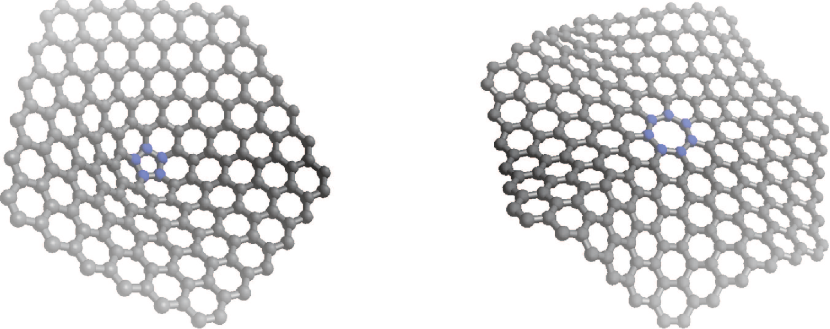
Figure 1: A conical surface made up by the inclusion of an one-pentagon apex ($\alpha<1$) (left) and a saddle-like surface made up by the inclusion of an one-heptagon apex ($\alpha>1$) on a honeycomb lattice (right).

The Gaussian curvature, which is related to a geometric singularity, is also known as a conical singularity and was shown to reveal subtle properties of quantum Hall states in [29]. The mean curvatures of the conical and saddle-like surfaces (both are not self-intersecting surfaces) differ by a signal,

$$\mathcal{H}=\frac{\sqrt{\pm(1-\alpha^{2})}}{2\alpha\rho},$$ (7)

where here, and in what follows, we shall use the convention that the upper sign is used for the conical surface and the lower sign is used for the saddle-like surface. This sign reversal occurs to be consistent with the fact that the saddle-like surface has a negative curvature [30]. Therefore, the geometric potential $V_{S}(r)$ reads

$$V_{S}(\rho)=\frac{1}{2M}\left[\mp\frac{1-\alpha^{2}}{4\alpha^{2}\rho^{2}}+\mathcal{K}\right].$$ (8)

We now introduce a magnetic flux tube parallel to the axis of the surface. In the background described by the metric (5), the vector potential, in the Coulomb gauge $\mathbf{\nabla}\cdot\mathbf{A}=0$, is written as

$$-QA_{i}=\epsilon_{ij}\frac{\phi r_{j}}{\alpha\rho^{2}},\qquad A_{3}=0,$$ (9)

where $\epsilon_{ij}=-\epsilon_{ji}$ with $\epsilon_{12}=+1$, $\phi=\Phi/\Phi_{0}$ is the flux parameter with $\Phi_{0}=2\pi/Q$. In this manner, by writing the surface component of the wave function as $\chi_{S}=e^{-iEt}\psi_{S}$, the Schrödinger equation (2) results in

$$-\frac{\partial^{2}\psi_{S}}{\partial\rho^{2}}-\frac{1}{\rho}\frac{\partial\psi_{S}}{\partial\rho}-\frac{1}{\alpha^{2}\rho^{2}}\left(\frac{\partial^{2}}{\partial\varphi^{2}}-\frac{2\phi}{i}\frac{\partial}{\partial\varphi}-\phi^{2}\right)\psi_{S}\\ \mp\frac{1-\alpha^{2}}{4\alpha^{2}\rho^{2}}\psi_{S}+\mathcal{K}\psi_{S}=k^{2}\psi_{S},$$ (10)

where $k^{2}=2ME$. We seek solutions of the form

$$\psi_{S}(\rho,\varphi)=e^{im\varphi}f_{m}(\rho),$$ (11)

where $f_{m}(\rho)$ satisfies the eigenvalue equation

$$hf_{m}(\rho)=k^{2}f_{m}(\rho),$$ (12)

with

$$h=h_{0}+\mathcal{K},$$ (13)

$$h_{0}=-\frac{d^{2}}{d\rho^{2}}-\frac{1}{\rho}\frac{d}{d\rho}+\frac{j^{2}}{\rho^{2}},$$ (14)

and

$$j^{2}=\frac{4(m+\phi)^{2}\mp(1-\alpha^{2})}{4\alpha^{2}},$$ (15)

is the effective angular momentum. We can observe from Eq. (15) that some combinations of the variables $m$, $\phi$ and $\alpha$ may lead to $j^{2}<0$, resulting $j$ being a complex number [18]. However, in this work, we shall only focus our attention on $\alpha$ values that satisfy the condition

$$4(m+\phi)^{2}>\pm(1-\alpha^{2}).$$ (16)

III The self-adjoint extension approach

The presence of the singular Gaussian curvature, $\mathcal{K}$, in the Hamiltonian $h$, as discussed above, turns it into a non-self-adjoint operator. The non-self-adjointness of $h$ stems from the fact that the $\mathcal{K}$ must be singular at the cone apex. Therefore, $h$ must be analyzed in the light of the self-adjoint extension approach. The self-adjoint extension approach is a well-known technique [28, 31, 32]. However, to be self-contained, in this section we briefly review the principal concepts and results of the self-adjoint extension approach.

Let us start by defining a self-adjoint operator. A densely defined linear operator $\mathcal{O}$ on a Hilbert space is said to be self-adjoint if it equals to its adjoint $\mathcal{O}^{\dagger}$. Then, two conditions must be fulfilled: (i) the domain of $\mathcal{O}$ coincides with the domain of its adjoint, $\mathcal{D}(\mathcal{O})=\mathcal{D}(\mathcal{O}^{\dagger})$; and (ii) the operator and its adjoint are equal in this domain, $\mathcal{O}=\mathcal{O}^{\dagger}$. As said above, $h$ is not self-adjoint. However, it is natural to think $h$ as a self-adjoint extension of $h_{0}$ given that fact that for smooth functions $\xi\in C_{0}^{\infty}(\mathbb{R}^{2})$ this two operators coincide at the origin, $h\xi(0)=h_{0}\xi(0)$ [33]. Indeed, from the general theory of the self-adjoint extensions, it is known that $h_{0}$ is self–adjoint only for $|j|\geq 1$, whereas for $|j|<1$ it is not self-adjoint, has deficiency indices $(1,1)$ and admits a one-parameter family of self-adjoint extensions [34]. Then, we have to extend the domain of $h_{0}$ to its deficiency subspace when $|j|<1$, which is spanned by the solutions of $h_{0}f_{\pm}=\pm ik_{0}^{2}f_{\pm}$, where $k_{0}$ is a real parameter introduced for dimensional reasons. As showed in [35], all the self-adjoint extensions of $h_{0}$ are parametrized by a boundary condition at the origin

$$\nu f_{0,j}=f_{1,j},$$ (17)

where the boundary values are

$$f_{0,j}={} \lim_{\rho\rightarrow 0^{+}}\rho^{|j|}f_{m}(\rho),$$

$$f_{1,j}={} \lim_{\rho\rightarrow 0^{+}}\frac{1}{\rho^{|j|}}\left[f_{m}(\rho)-f_{0,j}\frac{1}{\rho^{|j|}}\right],$$

and $\nu$ is the self-adjoint extension parameter defined in the range $-\infty<\nu\leq\infty$. The boundary condition in (17) describes $h_{0}$ plus a point interaction at the origin (i.e., $h$). The particular value $\nu=\infty$ is included in the range to represent the free Hamiltonian, which corresponds to the case of the flat space, $\alpha=1$, where the $\mathcal{K}$ strength vanishes and the Hamiltonian reduces to

$$h_{\rm AB}=-\frac{d^{2}}{d\rho^{2}}-\frac{1}{\rho}\frac{d}{d\rho}+\frac{(m+\phi)^{2}}{\rho^{2}}.$$ (18)

$h_{\rm AB}$ is the original AB Hamiltonian and, in this case, only regular solutions contribute to the problem [15]. On the other hand, it is not difficult to see that for $|\nu|<\infty$, this boundary condition permits the contribution of irregular solutions at the origin to the problem.

IV Scattering and bound states analysis

Now, we analyze the scattering and bound states for the system represented by the Hamiltonian $h$. We begin by writing the general solution of Eq. (12) for $r\neq 0$,

$$f_{m}(\rho)=a_{m}J_{|j|}(k\rho)+b_{m}J_{-|j|}(k\rho),$$ (19)

where $J_{\upsilon}(z)$ is the Bessel function of fractional order $\upsilon$. The coefficients $a_{m}$ and $b_{m}$ represent the contributions of the regular and irregular solutions at the origin, respectively. As in the case of the original AB Hamiltonian discussed above, it is very common in the literature discard the irregular solution due to the normalizability condition. However, due to the presence of the $\delta$ singularity in $h$, this cannot be done [36, 37]. We instead take into account both regular and irregular solutions and employ the boundary condition (17) to find out which irregular solutions are allowed by the self-adjoint extension. Thus, by applying the boundary condition (17) to the general solution in (19), it is possible to determine a relation between the coefficients $a_{m}$ and $b_{m}$. From this relation, we can conclude that $b_{m}$ must be zero for $|j|\geq 1$ and only the regular solution contributes to the wave function in this case. On the other hand, for $|j|<1$, we have the relation

$$b_{m}=-\Omega_{j}^{\nu}(k)a_{m},$$ (20)

where

$$\Omega_{j}^{\nu}(k)=\frac{k^{2|j|}\Gamma\left(1-|j|\right)\sin\left(|j|\pi\right)}{4^{|j|}\Gamma\left(1+|j|\right)\nu+k^{2|j|}\Gamma\left(1-|j|\right)\cos\left(|j|\pi\right)},$$ (21)

and $\Gamma(z)$ represents the gamma function. Therefore, the solution to the problem can be written as

$$f_{m}(\rho)=\begin{cases}a_{m}J_{|j|}(k\rho),&\text{for }|j|\geq 1\\ a_{m}\left[J_{|j|}(k\rho)-\Omega_{j}^{\nu}(k)J_{-|j|}(k\rho)\right],&\text{for }|j|<1.\end{cases}$$ (22)

Thus, we can see the contribution of the irregular solution for the wave function is controlled by the self-adjoint extension parameter. The $\mathcal{K}$ induces a short-range potential, then it is possible to analyze it in terms of scattering phase shifts. The phase shift, which measures how far the asymptotic scattering solution of the problem differs from the asymptotic free solution, can be obtained from the asymptotic expansion of the Bessel function in Eq. (22), and the result seems to be

$$\delta_{j}^{\nu}\left(k\right)=\begin{cases}\delta_{j}^{\rm AB},&\text{for }|j|\geq 1\\ \delta_{j}^{\rm AB}+\arctan\left[\Omega_{j}^{\nu}(k)\right],&\text{for }|j|<1.\end{cases}$$ (23)

where

$$\delta_{j}^{\rm AB}=\frac{\pi}{2}\left(|m|-|j|\right),$$ (24)

is the AB scattering phase shift in the curved space. It follows that the corresponding S–matrix (scattering matrix) is given by

$$S_{j}^{\nu}(k)={} e^{2i\delta_{j}^{\nu}(k)}$$

$$={} \begin{cases}e^{2i\delta_{m}^{\rm AB}},&\text{for }|j|\geq 1,\\ e^{2i\delta_{m}^{\rm AB}}\displaystyle\frac{1+i\Omega_{j}^{\nu}(k)}{1-i\Omega_{j}^{\nu}(k)}&\text{for }|j|<1.\end{cases}$$ (25)

Hence, the contribution of the irregular solution when $|j|<1$, which is controlled by the self-adjoint extension parameter $\nu$, causes a modification in the S–matrix when compared to the pure AB scattering [38]. Indeed, the result for the pure AB scattering is recovered if we set $\nu=\infty$ or $\alpha=1$, the result is $S_{m+\phi}^{\nu=\infty}=e^{2i\delta_{m+\phi}^{\rm AB}}$ for all $m$ values.

Another consequence of the contribution of the irregular solution is the presence of bound states. Bound states can be obtained from the poles of the S– matrix in the upper half of the $k$ complex plane. From Eq. (25), it is easy to see that the poles come from $i\Omega_{j}^{\nu}(i\kappa)=1$, where we made the substitution $k\to i\kappa$, $\kappa=\sqrt{-2ME_{b}}$ and $E_{b}$ is the bound state energy. Therefore, the explicit expression for the bound state energy is

$$E_{b}=-\frac{2}{M}\left[-\nu\frac{\Gamma(1+|j|)}{\Gamma(1-|j|)}\right]^{\frac{1}{|j|}},$$ (26)

for $|j|<1$ and the pole occurs only for negative values of $\nu$. Energy (26) is similar to the expression for the bound state energy obtained in Ref. [39], where the authors studied the contact interactions of anyons. We can also write down the scattering amplitude $f(k,\theta)$ in terms of the S–matrix:

$$f(k,\theta)={} \frac{1}{\sqrt{2\pi ik}}\sum_{m=-\infty}^{\infty}\left[S_{j}^{\nu}(k)-1\right]e^{im\theta}$$

$$={} \frac{1}{\sqrt{2\pi ik}}\Bigg{\{}\sum_{m\in\{|j|\geq 1\}}\left(e^{2i\delta_{m}^{\rm AB}}-1\right)e^{im\theta}$$

$$+\sum_{m\in\{|j|<1\}}\left[e^{2i\delta_{m}^{\rm AB}}\frac{1+i\Omega_{j}^{\nu}(k)}{1-i\Omega_{j}^{\nu}(k)}-1\right]e^{im\theta}\Bigg{\}}.$$ (27)

We can observe that the scattering amplitude has a dependence on the energy that goes beyond the usual energy scale which is, in the non-relativistic domain, set by $1/k$ [40]. This additional energy dependence comes from the singularity which arises from the geometric potential. In other words, the singularity promoted by the localized curvature, which is a conical topological defect, enhance the energy dependence of the scattering amplitude.

IV.1 Discussion

In Ref. [14], the authors studied the classical and quantum scattering on a conical surface in (2+1) dimensions. They considered an intrinsic conical geometry leading to a Hamiltonian which do not include the geometric potential, $V_{S}(r)$. Their result for the scattering phase shift differs from our when we set $\phi=0$. This difference is solely due to the presence of the geometric potential. Moreover, they do not find bound states. The presence of bound states in our system is also a consequence of the geometric potential, which arises from da Costa’s approach. So here we can see an observable difference between the 2D quantum mechanics on a conical surface and the 3D quantum mechanics constrained to a 2D embedded conical surface.

In the light of the constraint in Eq. (16), in the case of a conical surface, $\alpha<1$, the system does not have bound states when $\phi=0$. This is because of the effective angular momentum is always outside the range $|j|<1$ for all values of $m$. So, only the regular solution contributes to the problem. On the other hand, for $\alpha>1$, there are values of $m$ for which $|j|<1$, and there are bound states.

The fact that the scattering phase shift and the bound state energy are dependent on the self-adjoint extension parameter could appear strange at first. However, it is possible to show by using another self-adjoint approach, based on regularization of the $\delta$ potential [31, 32], that the self-adjoint extension parameter can be expressed in terms of physical parameters

$$\nu=-\frac{1}{r_{0}^{2|j|}}\left(\frac{1-\alpha+\alpha|j|}{1-\alpha-\alpha|j|}\right),$$ (28)

where $r_{0}$ is a very small radius which comes from the regularization of the $\delta$ function. This relation is valid only for $\nu<0$, because only for negative values of the self-adjoint extension parameter we can have simultaneously bound and scattering states which allow us to derive this relation.

V Conclusion

We have thus explored the scattering scenario for the problem of a spinless charged particle constrained to move on a curved surface, with positive and negative curvatures, in the presence of the AB flux. The particle is confined to move on the surface using the thin-layer procedure proposed by da Costa [2]. The procedure gives rise to a geometric potential with $\delta$ function singularity at the origin, which is related to the tip of the conical surface. Due to this singularity, the Hamiltonian of the system is not self-adjoint for all possible values of the effective angular momentum $j$. So, a suitable boundary condition, which comes from the theory of the self-adjoint extensions was employed. We have shown that this boundary condition allows the contribution of irregular solutions at the origin for $|j|<1$. As a result, the phase shift, S-matrix and scattering amplitude are modified when compared with the pure AB scattering results. In particular, due to the inclusion of irregular solutions, our scattering results show additional energy dependence. Moreover, from the poles of the S–matrix, an expression for the bound state is obtained. Finally, we have shown that the origin of this energy dependence is solely due to the effects of curvature. This comes from the geometric potential that arises from da Costa’s thin-layer approach. Therefore, we can conclude that the additional dependence on the energy of the scattering amplitude $f(k,\theta)$ is solely due to the effects of localized curvature.