An Asynchronous Task-based Fan-Both Sparse Cholesky Solver

Abstract

Systems of linear equations arise at the heart of many scientific and engineering applications. Many of these linear systems are sparse; i.e., most of the elements in the coefficient matrix are zero. Direct methods based on matrix factorizations are sometimes needed to ensure accurate solutions. For example, accurate solution of sparse linear systems is needed in shift-invert Lanczos to compute interior eigenvalues. The performance and resource usage of sparse matrix factorizations are critical to time-to-solution and maximum problem size solvable on a given platform.

In many applications, the coefficient matrices are symmetric, and exploiting symmetry will reduce both the amount of work and storage cost required for factorization. When the factorization is performed on large-scale distributed memory platforms, communication cost is critical to the performance of the algorithm. At the same time, network topologies have become increasingly complex, so that modern platforms exhibit a high level of performance variability. This makes scheduling of computations an intricate and performance-critical task.

In this paper, we investigate the use of an asynchronous task paradigm, one-sided communication and dynamic scheduling in implementing sparse Cholesky factorization (symPACK) on large-scale distributed memory platforms. Our solver symPACK relies on efficient and flexible communication primitives provided by the UPC++ library. Performance evaluation shows good scalability and that symPACK outperforms state-of-the-art parallel distributed memory factorization packages, validating our approach on practical cases.

I Introduction

Symmetric positive definite systems of linear equations arise in the solution of many scientific and engineering problems. Efficient solution of such linear system is important for the overall performance of the application codes. In this paper, we consider direct methods for solving a sparse symmetric positive definite linear system, which are based on Cholesky factorization. While direct methods can be expensive for large matrices, in terms of execution times and storage requirement when compared to iterative methods, they have the advantage that they terminate in a finite number of operations. Also, direct methods can handle linear systems that are ill conditioned or the situation when there are many multiple right-hand sides. An example of ill-conditioned linear systems is in the computation of interior eigenvalues of a matrix using the shift-invert Lanczos algorithm.

We propose a new implementation of sparse Cholesky factorization using an asynchronous task paradigm. We introduce a parallel distributed memory solver called symPACK. By using a task-based formalism and dynamic scheduling techniques within a node, symPACK achieves good strong scaling on modern supercomputers.

An outline of the paper is as follows. In Section II, we provide some background on sparse Cholesky factorization. In Section III, we present our implementation in symPACK. The asynchronous paradigm is described in Section IV. Some numerical results are presented in Section V, followed by some concluding remarks in Section VI

II Background on Cholesky factorization

In the following, we give some background on Cholesky factorization and how symmetry and sparsity can be taken into account. We first review the basic Cholesky algorithm for dense matrices and then detail how it can be modified to handle sparse matrices efficiently. We also present fundamental notions on sparse matrix computations before reviewing the work related to sparse Cholesky factorization.

II-A The basic algorithms

Let $\mathbf{{A}}=[a_{i,j}]$ be an $n$-by-$n$ symmetric positive definite matrix. The Cholesky algorithm factors the matrix $\mathbf{{A}}$ into

$$\mathbf{{A}}=\mathbf{{L}}\mathbf{{L}}^{T},$$ (1)

where $\mathbf{{L}}=[\ell_{i,j}]$ is a lower triangular matrix, and $\mathbf{{L}}^{T}$ is the transpose of $\mathbf{{L}}$ and is upper triangular. The factorization thus allows symmetry to be exploited, since only $\mathbf{{L}}$ needs to be computed and saved.

for column $j=1$ to $n$ do

       $\ell_{j,j}=\sqrt{a_{j,j}}$

       for row $i=j+1$ to $n$ do

             $\ell_{i,j}=a_{i,j}/\ell_{j,j}$

            

       end for

      

       for column $k=j+1$ to $n$ do

             for row $i=k$ to $n$ do

                   $a_{i,k}=a_{i,k}-\ell_{i,j}\cdot\ell_{k,j}$

                  

             end for

            

       end for

      

end for

Algorithm 1 Basic Cholesky algorithm

The basic Cholesky factorization algorithm, given in Alg. 1, can be described as follows:

1. Current column $j$ of $\mathbf{{L}}$ is computed using column $j$ of $\mathbf{{A}}$.

2. Column $j$ of $\mathbf{{L}}$ is used to update the remaining columns of $\mathbf{{A}}$.

If $\mathbf{{A}}$ is a dense matrix, then every column $k$, $k>j$, is updated.

Once the factorization is computed, the solution to the original linear system can be obtained by solving two triangular linear systems using the Cholesky factor $\mathbf{{L}}$.

II-B Cholesky factorization of sparse matrices

For large-scale applications, $\mathbf{{A}}$ is often sparse, meaning that most of the elements of $\mathbf{{A}}$ are zero. When the Cholesky factorization of $\mathbf{{A}}$ is computed, some of the zero entries will turn into nonzero (due to the subtraction operations in the column updates; see Alg. 1). The extra nonzero entries are referred to as fill-in. For in-depth discussion of sparse Cholesky factorization, the reader is referred to [1].

Following is an important observation in sparse Cholesky factorization. It is expected that the columns of $\mathbf{{L}}$ will become denser and denser as one moves from the left to the right. This is due to the fact that the fill-in in one column will result in additional fill-in in subsequent columns. Thus, it is not uncommon to find groups of consecutive columns that eventually share essentially the same zero-nonzero structure. Such a group of columns is referred to as a supernode. To be specific, if columns $i$, $i+1$, $\cdots$, $j$ form a supernode, then the diagonal block of these columns will be completely dense, and row $k$, $j+1\leq k\leq n$, within the supernode is either entirely zero or entirely nonzero.

Fill-in entries and supernodes of a sample symmetric matrix are depicted in Figure 1a. In this example, 10 supernodes are found. Fill-in entries are created in supernode 8 because of the nonzero entries in supernode 6.

(a)

(b) Supernodal elimination tree of matrix $\mathbf{{A}}$

Figure 1: Sparse matrix $\mathbf{{A}}$ partitioned into supernodes, denotes the $i$-th supernode. represents original nonzero elements in $\mathbf{{A}}$, while + denotes fill-in entries. Colors correspond to the 4 distributed memory nodes on which supernodes are mapped in a 1D-cyclic way.

The elimination tree of $\mathbf{{A}}$ (or $\mathbf{{L}}$) is a very important and useful tool in sparse Cholesky factorization. It is an acyclic graph that has $n$ vertices $\{v_{1},v_{2},\cdots,v_{n}\}$, with $v_{i}$ corresponding to column $i$ of $\mathbf{{A}}$. Suppose $i>j$. There is an edge between $v_{i}$ and $v_{j}$ in the elimination tree if and only if $\ell_{ij}$ is the first off-diagonal nonzero entry in column $j$ of $\mathbf{{L}}$. Thus, $v_{i}$ is called the parent of $v_{j}$ and $v_{j}$ is a child of $v_{i}$. The elimination tree contains a lot of information regarding the sparsity structure of $\mathbf{{L}}$ and the dependency among the columns of $\mathbf{{L}}$. See [2] for details.

An elimination tree can be expressed in terms of supernodes rather than column. In such a case, it is referred to as a supernodal elimination tree. An example of such tree is depicted in Figure 1b.

II-C Scheduling in parallel sparse Cholesky factorization

In the following, we discuss scheduling of the computation in the numerical factorization. The only constraints that have to be respected are the numerical dependencies among the columns: column $k$ of $\mathbf{{A}}$ has to be updated by column $j$ of $\mathbf{{L}}$, for any $j<k$ such that $\ell_{k,j}\neq 0$, but the order in which the updates occur is mathematically irrelevant, as long as the updates are performed before column $k$ of $\mathbf{{A}}$ is factored. There is therefore significant freedom in the scheduling of computational tasks that factorization algorithms can exploit.

For instance, on sequential platforms, this has led to two well-known variants of the Cholesky factorization algorithm: left-looking and right-looking schemes, which have been introduced in the context of dense linear algebra [3]. In the left-looking algorithm, before column $k$ of $\mathbf{{A}}$ is factored, all updates coming from columns $i$ of $\mathbf{{L}}$ such that $i<k$ and $\ell_{k,i}\neq 0$ are first applied. In that sense, the algorithm is “looking to the left” of column $k$. In right-looking, after a column $k$ has been factored, every column $i$ such that $k<i$ and $\ell_{i,k}\neq 0$ is updated by column $k$. The algorithm thus “looks to the right” of column $k$.

Distributed memory platforms add the question of where the computations are going to be performed. Various parallel algorithms have been proposed in the literature for Cholesky factorization, such as MUMPS [4], which is based on the multifrontal approach (a variant of right-looking), and PASTIX [5], which is left-looking.

In [6], the author classifies parallel Cholesky algorithms into three families: fan-in, fan-out and fan-both.

The fan-in family includes all algorithms such that all updates from a column $k$ to other columns $i$, for $k<i$ such that $\ell_{i,k}\neq 0$, are computed on the processor owning column $k$. When one of these columns, say $i$, will be factored, the processor owning $i$ will have to “fan-in” (or collect) updates from previous columns.

The fan-out family includes algorithms that compute updates from column $k$ to columns $i$, for $k<i$ such that $\ell_{k,i}\neq 0$, on processors owning columns $i$. This means that the processor owning column $k$ has to “fan-out” (or broadcast) column $k$ of the Cholesky factor.

The fan-both family generalizes these two families to allow these updates to be performed on any processors. This family relies on computation maps to map computations to processors.

In the rest of the paper, we will use the term fan-both algorithm as a shorthand to refer to an algorithm belonging to the fan-both family (and similarly for fan-in and fan-out).

III A versatile parallel sparse Cholesky algorithm

As mentioned in the previous section, there are many ways to schedule the computations as long as the precedence constraints are satisfied. The Cholesky factorization in symPACK is inspired by the fan-both algorithm. This leads to a high level of versatility and modularity, which allows symPACK to adapt to various platforms and network topologies.

III-A Task-based formulation

Both fan-both and symPACK involve three types of operations: factorization, update, aggregation. We let $\mathbf{{A}}$ be an $n$-by-$n$ matrix, and denote these tasks using the following notation:

• Factorization $F_{i,i}$: compute column $i$ of the Cholesky factor.

• Update $U_{i,j}$: compute the update from $\ell_{j:n,i}$ to column $j$, with $i<j$ such that $\ell_{j,i}\neq 0$, and put it to an aggregate vector $t^{i}_{j}$.

• Aggregation $A_{j,j}$: apply all aggregate vectors $t^{i}_{j}$ from columns $i<j$, with $\ell_{j,i}\neq 0$, to column $j$.

An example of dependencies among these tasks for three columns $j$, $i$ and $h$, with $j<i$ and $j<h$, is depicted in Figure 2. After column $j$ has been factored, its updates to dependent columns $i$ and $h$ can be computed. This corresponds to tasks $U_{j,i}$ and $U_{j,h}$. Note that both these tasks require $\ell_{j:n,j}$, which has to be fanned-out to these two tasks. After these two tasks have been processed, $t^{j}_{i}$ and $t^{j}_{h}$ have been computed. $A_{i,i}$ can now be updated using $t^{j}_{i}$, after which $F_{i,i}$ is ready to be executed. After that, the task $U_{i,h}$, which produces $t^{i}_{h}$, can be executed. The two aggregate vectors $t^{j}_{h}$ and $t^{i}_{h}$ are then applied on column $h$ during the execution of task $A_{h,h}$, requiring aggregate vectors to be fanned-in. Finally, task $F_{h,h}$ can be processed. As can be observed, fan-both indeed involves data exchanges that can be observed in either fan-in or fan-out.

Figure 2: fan-both task dependencies for three columns $j$, $i$ and $h$

III-B Parallel algorithm and computation maps

We now describe fan-both in a parallel setting. We assume a parallel distributed memory platform with $P$ processors ranging from $p_{1}$ to $p_{P}$. We assume that $\mathbf{{A}}$ and $\mathbf{{L}}$ are cyclically distributed by supernodes of various sizes in a 1D way, as depicted in Figure 1a. The maximum supernode size is limited to 150 columns. This has the benefit of allowing a good load balancing of nonzero entries and computation per processor, although communication might not achieve optimal load balance. An example of such a distribution using 4 distributed memory nodes, or processors, is depicted in Figure 1a.

Ashcraft [6] introduces the concept of computation maps to guide the mapping of tasks onto processors. A mapping $\mathcal{M}$ is a two-dimensional grid that “extends” to the matrix size (i.e., $n$-by-$n$). Values represent node ranks computed using a closed-form generator expression. Therefore, the $n$-by-$n$ grid is not explicitly stored. A mapping is said to be $1$-by-$P$ when 1 rank is found in each column of $\mathcal{M}$, $P$-by-1 when $P$ distinct values are found in every column and $\sqrt{P}$-by-$\sqrt{P}$ when $\sqrt{P}$ distinct ranks are found on each row and column.

A computation map $\mathcal{M}$ is used to map the tasks as follows:

• Tasks $A_{i,i}$ and $F_{i,i}$ are mapped onto node $p_{\mathcal{M}_{i,i}}$

• Tasks $U_{i,j}$ is mapped onto node $p_{\mathcal{M}_{j,i}}$

In a parallel setting, aggregate vectors can be further accumulated on each node to reflect the updates of all local columns residing on a given node $p_{i}$ to a given column $j$. We let $a^{(p_{i})}_{j}$ be such an aggregate vector. We have:

$$a^{(p_{i})}_{j}=\sum_{\begin{array}[]{c}\forall i<n~{}\textnormal{on}~{}p_{i}\\ i~{}\textnormal{updates}~{}j\end{array}}t^{i}_{j}.$$

Given a task mapping strategy $\mathcal{M}$, it is important to note that the factor columns $\ell_{i:n,i}$, $\forall i$, $1\leq i\leq n$ need to be sent to at most the number of distinct node ranks present in the lower triangular part of column $i$ of $\mathcal{M}$. Aggregate vectors need to be sent to the number of distinct ranks in the lower triangular part of row $i$ of $\mathcal{M}$.

(a)

(b)

(c)

Figure 3: Three different computation maps, corresponding to algorithms in fan-in, fan-out and fan-both

In [6], the author discusses the worst case communication volume depending on which computation map is used. The $\sqrt{P}$-by-$\sqrt{P}$ maps involve at most $\sqrt{P}$ nodes in each communication step, while each step involves at most $P$ nodes for either $P$-by-1 or 1-by-$P$ computation maps. The volume is directly impacted by the number of nodes participating to each communication step. However, the $\sqrt{P}$-by-$\sqrt{P}$ maps require two kinds of messages to be exchanged (i.e. both factors and aggregate vectors) while 1-by-$P$ or $P$-by-1 only require one type of message. The latency cost is therefore higher for $\sqrt{P}$-by-$\sqrt{P}$ computation maps.

Various formulations of the Cholesky factorization can generally be described by a fan-both algorithm with appropriate computation maps. For instance, fan-in and fan-out are good examples, as illustrated by Figure 3. Our symPACK also uses these computation maps but it is not restricted to such task assignments. This flexible design will allow us to derive and evaluate a wider range of task mapping and scheduling strategies.

III-C Impact of communication strategy

Without loss of generality, parallel distributed memory algorithms perform communication following two strategies. A data transfer happening between two processors (or nodes) $p_{\textnormal{source}}$ and $p_{\textnormal{target}}$ can be performed the following ways:

• $p_{\textnormal{source}}$ sends the data to $p_{\textnormal{target}}$ as soon as the data is available using a push strategy,

• $p_{\textnormal{target}}$ gets the data from $p_{\textnormal{source}}$ as soon as data is required using a pull strategy.

These two strategies will be explained in detail below.

Another very important characteristic of communication protocols is whether a communication primitive is two-sided or one-sided. The former requires $p_{\textnormal{source}}$ to issue a send operation and $p_{\textnormal{target}}$ to issue a matching receive operation. Such strategy is employed in most MPI applications. The latter strategy can be employed in two ways, and relies on the fact that the communication library is able to write/read to/from a remote memory location. Either $p_{\textnormal{source}}$ puts directly the data into $p_{\textnormal{target}}$’s memory, or $p_{\textnormal{target}}$ gets the data directly from $p_{\textnormal{source}}$’s memory. This type of communication have been introduced in MPI-2 and refined in MPI-3, and is also available in other libraries such as GASNet.

In the following, we discuss those strategies and their corresponding implications in the context of the sparse Cholesky factorization, and more generally in the context of direct sparse solvers. Two kinds of messages can be exchanged throughout the factorization: factors and aggregate vectors. The first type of messages corresponds to the entries in a column after it has been factorized, or in other words, to a portion of the output data of the algorithm. The second type of messages is a temporary buffer in which a given $p_{\textnormal{source}}$ will accumulate all its updates to a remote target column residing on $p_{\textnormal{target}}$.

In the next two paragraphs, we suppose that two tasks $T_{i,j}$ and $T_{j,j}$ are respectively mapped onto two processors $p_{\textnormal{source}}$ and $p_{\textnormal{target}}$. Task $T_{j,j}$ depends on data produced by task $T_{i,j}$. Let $M_{i,j}$ denote that data.

Push strategy

First, $p_{\textnormal{source}}$ computes task $T_{i,j}$. As soon as it is done processing that task, it sends $M_{i,j}$ to processor $p_{\textnormal{target}}$. When processor $p_{\textnormal{target}}$ selects task $T_{j,j}$ to be executed, the first thing done is to post a receive request, and wait until $M_{i,j}$ has been fetched. Once it is received, task $T_{j,j}$ can be processed.

Pull strategy

Let us now consider the pull strategy. Processor $p_{\textnormal{source}}$ processes task $T_{i,j}$ and produces $M_{i,j}$. Later on, processor $p_{\textnormal{target}}$ selects task $T_{j,j}$. It first sends a message to processor $p_{\textnormal{source}}$, requesting $M_{i,j}$ to be sent to processor $p_{\textnormal{target}}$. Once this transfer is completed, task $T_{j,j}$ can be processed.

The key difference between the push strategy and the pull strategy is therefore which processor has the responsibility to initiate the data exchange.

III-D Asynchronous communications and deadlock situations

In the following, we discuss the use of asynchronous communication primitives in sparse matrix solvers, and more specifically in the case of Cholesky factorization. Asynchronous communications, or non-blocking communications, are often used in parallel applications in order to achieve good strong scaling and deliver high performance.

In some situations though, asynchronous communications must be used with care. Communication libraries have to resort to a certain number of buffers to perform multiple asynchronous communications concurrently. However, the space for these buffers is a limited resource, and a communication library will certainly run out of buffer space if too many asynchronous communications are performed concurrently. In such a case, the communication primitives become blocking and deadlock might occur. This latter case corresponds to the situation in which each processor has only one send buffer and one receive buffer.

Let us consider a task graph and more precisely the simpler case where that task graph is a directed tree, and analyze it in the context of matrix computation. Let us also suppose that operations are performed on entire columns of an input matrix. Let us denote:

• $\mathbf{{A}}$ an input matrix of dimension $n$ on which operations are going to be applied to columns.

• $\mathcal{C}$ the set of columns in $\mathbf{{A}}$ and distributed onto $P$ processors in a cyclic way. We have $\forall i\in\mathcal{C},i\leq n$.

• $\mathcal{T}=(V,E)$: a task tree, where $V$ is the set of vertices in the tree and $E$ the set of directed edges between vertices in $E$.

• $T_{i,j}\in V$ a task from a source column $i\in\mathcal{C}$ to a target column $j\in\mathcal{C},i\leq j$, of matrix $\mathbf{{A}}$. Let us assume that column $j$ is modified after $T_{i,j}$ has been processed.

• $M_{i,j}=(T_{i,j},T_{j,k})\in E$ a dependency between two tasks $T_{i,j}$ and $T_{j,k}\in V$. It corresponds to a communication if tasks are not mapped onto the same processor.

For sparse Cholesky factorization, such a task tree can be derived from the elimination tree of matrix $\mathbf{{A}}$. We suppose that this elimination tree has been labeled in a post-order fashion, which is generally the case. Therefore, every edge $(T_{i,j},T_{j,k})$ in $E$ has to respect the constraint $i\leq j\leq k$.

Suppose that each processor has only one send buffer and one receive buffer, and that processors will push, or send, the newly produced data as soon as it has been produced. Let us also assume that prior to executing a task, the incoming data has to be received.

Such a task tree is depicted in Figure 4, with different colors corresponding to distinct processors. Let us describe how such a tree is processed by the $P$ processors.

Figure 4: A task tree where deadlock happens. Green solid arrows correspond to send operations (and their local order on each processor). Red dashed arrows correspond to receive operations (and their local order).

First, each of the $P$ processors executes one task $T_{i,P+1},1\leq i\leq P$, of the bottom level. Processors $p_{2}$ to $p_{P}$ send their respective data to processor $p_{1}$, which receives each message one by one in a sequential way.

All processors can now compute tasks $T_{P+i,3P+2},1\leq i\leq P$, and then send their respective data to processor $p_{2}$ on which task $T_{3P+2,3P+2}$ has been assigned. This consumes the send buffer of all processors but processor $p_{2}$.

Processor $p_{1}$ then computes task $T_{2P+1,2P+2}$ in the rightmost branch of the tree. It cannot send the data because the send buffer is currently occupied. Processor $p_{2}$ is waiting for the incoming data to task $T_{2P+2,2P+3}$, which cannot be sent by $p_{1}$. Hence a deadlock situation.

In order to avoid this kind of situation, tasks and messages can be scheduled in the following way:

• Process tasks $T_{i,j}\in V$ in non-decreasing order of target column $j$, then in non-decreasing order of source column $i$.

• Send message $M_{i,j}\in E$ in non-decreasing order of target column $j$, then in non-decreasing order of source column $i$ and only if $M_{i,j}<T_{i^{\prime},j^{\prime}}$ with respect to this ordering where $T_{i^{\prime},j^{\prime}}$ is the next task scheduled onto this processor.

This problem has also been observed in [7] in the context of multifrontal factorization, in which a similar criterion has to be used.

IV Asynchronous task-based formulation

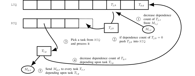
Figure 5: Task scheduling in symPACK. Update of task dependence in LTQ. Dynamic scheduling of local tasks in RTQ.

Modern platforms can be subject to high performance variability, and it is hard to derive an accurate model of such platforms. Obtaining good static scheduling strategies is therefore difficult. For scheduling purposes, an application is often modeled using Directed Acyclic Graphs (or DAGs). Computations are modeled as tasks, and represented by vertices in the graph while dependencies between tasks are represented by the edges. In the context of sparse matrix computations, there is no fixed task graph for a particular numerical kernel. The task graph is inherently depending upon the structure of the sparse matrix on which the computation is going to be performed. This makes the use of advanced static scheduling techniques even harder to apply.

This motivated us to rely on a dynamic scheduling approach instead, which is by nature more amenable to cope with performance variations and incomplete knowledge of the task graph. Even when the task graph is known, which is the case in sparse matrix factorizations, task completions are hard to predict on a parallel platform and dynamic scheduling is an efficient way to deal with this issue. We propose the following data structure, where each processor has:

• a local task queue (LTQ), containing all the tasks statically mapped onto this processor and awaiting execution,

• a ready task queue (RTQ), containing all the tasks for which precedence constraints have been satisfied and that can therefore be processed.

This is illustrated in Figure 5.

A task $T_{s,t}$ is represented by a source supernode $s$ and a target supernode $t$ on which computations have to be applied. Each task also has an incoming dependency counter, initially set to the number of incoming edges.

As symPACK implements a factorization similar to fan-both, three types of tasks have to be dealt with. Similarly, a message $M_{s,t}$ exchanged to satisfy the dependence between tasks mapped onto distinct processors is labeled by the source supernode $s$ of the receiving task and the target supernode $t$ of the receiving task.

The overall mechanism that we propose is the following: whenever a task is completed, processors owning dependent tasks are notified that new input data is now available.

As soon as a processor is done with its current computation, it periodically handles these incoming notifications by issuing one-sided gets. This get operation can either be a non-blocking communication or a blocking communication. The incoming dependency counter of the corresponding task is decremented when the communication has been completed. This corresponds to a strategy similar to the pull strategy discussed earlier, the only difference being that $p_{\textnormal{source}}$ directly notifies $p_{\textnormal{target}}$ rather than $p_{\textnormal{target}}$ periodically requesting data to $p_{\textnormal{source}}$.

When a task from the LTQ has all its dependencies satisfied (i.e., when its dependency counter reaches zero) then it is moved to the RTQ, and is now ready for execution. The processor then picks a task from the RTQ and executes it. If multiple tasks are available in the RTQ, then the next task that will be processed is picked according to a dynamic scheduling policy. As a first step, we use the same criterion for picking a task in the RTQ than the criterion that prevents deadlocks. Evaluating different scheduling policies will be the subject of a future analysis.

IV-A Data-driven asynchronous communication model

Communications are becoming a bottleneck in most scientific computing applications. This is even more true for sparse linear algebra kernels, which often exhibit a higher communication to computation ratio. Moreover, modern parallel platforms have to exploit interconnects that are more complex than in the past, and often display a deeper hierarchical structure. Larger scale also has a side-effect which can be observed on most modern platforms: performance variability. In the following, we propose a communication protocol for our parallel sparse Cholesky implementation that allow the communications to drive the scheduling. This is a crucial piece toward an Asynchronous Task execution model.

We use the UPC++ PGAS library [8, 9] for communicating between distributed memory nodes. UPC++ is built on top of GASNet [10], and introduces several parallel programming features useful for our implementation.

First, it provides global pointers for accessing memory locations on remote nodes. Using the get and put functions, one can transfer the data between two nodes in a one-sided way. Moreover, these transfers are handled by RDMA calls, and are therefore generally performed without interrupting the remote processor. Using this concept of global pointers, UPC++ also allows us to allocate and deallocate memory on a node from a remote node.

Another useful feature is the ability to perform remote asynchronous function calls. A processor can submit a function for execution on a remote node. It gets pushed into a queue that the remote processor executes when calling the UPC++ progress function.

Figure 6: Data exchange protocol in symPACK. Notifications are performed using UPC++ asynchronous tasks, actual data is fetched with one-sided get.

We consider a data notification and communication process which is heavily based on these two features of UPC++. This process is depicted in Figure 6. Let us suppose that at the end of a computation, $p_{\textnormal{source}}$ has produced some data that needs to be sent out to $p_{\textnormal{target}}$.

First, $p_{\textnormal{source}}$ notifies $p_{\textnormal{target}}$ that some data has been produced by sending it a pointer ptr to the data along with some meta-data meta. This is done by doing an asynchronous function call to a signal(ptr,meta) function on $p_{\textnormal{target}}$ directly from $p_{\textnormal{source}}$, and is referred to as step 1 in the diagram.

When $p_{\textnormal{target}}$ finishes its current computation, it calls a poll function (step 2), whose main role is to watch for incoming communications and do the book-keeping of task dependencies. This function resorts to UPC++ progress function to execute all asynchronous calls to the signal(ptr,meta) function, which enqueues ptr and meta into a list. This corresponds to steps 3 and 4. The next step in the poll function is to go through that list of global ptr and issue a get operation to pull the data (step 5). Note that this get can be asynchronous, but for the sake of simplicity, we suppose a blocking get operation here. Once the get operation is completed, the poll function updates the dependencies of the every task $T_{m}$ that will be using this data (which can be found by looking at the meta-data meta). If all dependencies of a task are met, that task is moved into the list of ready-tasks RTQ (at step 6).

Finally, $p_{\textnormal{target}}$ resumes its work by selecting a task from RTQ and run it.

As mentioned before, two types of data are encountered in Cholesky factorization: factors and aggregate vectors. Factors represent the output of the algorithm. The procedure described in Figure 6 can be applied to these factors in a straightforward way. Aggregate vectors, however, are temporary data. Hence, they need to be deleted when not required anymore; that is after step 5 of the process has been completed. UPC++ allows a process to deallocate memory on a remote process using a global pointer to that memory zone. Therefore, when dealing with aggregate vectors, $p_{\textnormal{target}}$ will deallocate the data pointed by ptr on $p_{\textnormal{source}}$ after it is done fetching it, without interrupting $p_{\textnormal{source}}$.

V Performance evaluation

In this section, we present the performance of the sparse Cholesky factorization implemented in our solver symPACK. Our experiments are conducted on the NERSC Edison supercomputer, which is based on Cray XC30 nodes. Each node has two Intel(R) Xeon(R) CPU E5-2695 v2 “Ivy bridge” processors with 12 cores running at 2.40GHz and 64GB of memory [11].

We evaluate the performance of symPACK, our parallel asynchronous task-based sparse Cholesky implementation using a set of matrices from the University of Florida Sparse Matrix Collection [12]. A description of each matrix can be found in Table I.

In this paper, we analyze the performance of symPACK in a distributed memory setting only. Therefore, all experiments are conducted without multi-threading (which is commonly referred to as “flat-MPI”).

For sparse Cholesky factorization, the amount of fill-in that occurs depends on where the nonzero elements are in the matrix. Permuting (or ordering) the matrix symmetrically changes its zero-nonzero structure, and hence changes the amount of fill-in in the factorization process. In our experiments, a fill-reducing ordering computed using Scotch [13] is applied to the original matrix. The Scotch library contains an implementation of the nested dissection algorithm [14] to compute a permutation that reduces the number of fill-in entries in the Cholesky factor.

Matrices from UFL sparse matrix collection Name Type $n$ $nnz(A)$ $nnz(L)$ boneS10 3D trabecular bone 914,898 20,896,803 318,019,434 bone010 3D trabecular bone 986,703 24,419,243 1,240,987,782 G3_circuit Circuit simulation problem 1,585,478 4,623,152 107,274,665 audikw_1 Symmetric rb matrix 943,695 39,297,771 1,221,674,796 af_shell7 Sheet metal forming, positive definite 504,855 9,042,005 104,329,190 Flan_1565 3D model of a steel flange, hexahedral finite elements 1,564,794 57,865,083 1,574,541,576

TABLE I: Characteristics of matrices used in the experiments

V-A Impact of communication and scheduling strategy

First, we aim at characterizing the impact of the communication strategy used during Cholesky factorization. We also aim at evaluating the impact of the dynamic scheduling described in Section  IV. To this end, we conduct a strong scaling experiment using the boneS10 matrix from the University of Florida Sparse Matrix collection [12]. Run times are averaged out of two runs. Results are depicted in Figure 7, with error bars representing standard deviations. In this experiment, three variants of symPACK are compared: Push, Pull and Pull + dynamic scheduling.

The Push variant of symPACK is based on a two-sided push communication protocol implemented using MPI. It uses the scheduling constraints introduced in Section III-D to prevent deadlocks. These constraints apply to both computations and communications.

The Pull variant implements a one-sided pull communication protocol using UPC++, but relieves the constraints on communications while still respecting the constraints on computations. As a result, both Push and Pull executes the same static schedule for computations, but organize communication in two different ways.

Figure 7: Impact of communication strategy and scheduling on symPACK performance

We observe in Figure 7 that the Pull variant of symPACK outperforms the Push variant. This confirms that the communication protocol described in Section IV-A and that relies on UPC++ to perform the one-sided communications displays a negligible overhead compared to a two-sided communication strategy using MPI.

This performance difference confirms that the sorting criterion that needs to be applied on both tasks and outgoing communications when using a push strategy also significantly constrains the schedule. Removing the constraints on how communications are scheduled while avoiding still deadlocks through the use of the Pull strategy allows to achieve a better scalability.

This trend is further improved by using a dynamic scheduling policy in conjunction with the Pull strategy. This confirms the dynamic scheduling as described in Section IV is a good way to improve scalability in the context of sparse matrix computations. In the rest of the paper, results corresponding to symPACK will correspond to the Pull + dynamic scheduling variant.

V-B Strong scaling

In the next set of experiments, we evaluate the strong scaling of our sparse symmetric solver symPACK. We compare its performance to two state-of-the-art parallel symmetric solvers: MUMPS 5.0 [4] and PASTIX 5.2.2 [5]. The package MUMPS is a well-known sparse solver based on the multifrontal approach and that implements a symmetric factorization. The code PASTIX is based on a right-looking supernodal formulation.

We also provide the run times achieved by SuperLU_DIST 4.3 [15, 16] as a reference. Note that SuperLU_DIST is not a symmetric code and therefore requires twice as much memory and floating point operations (if the columns are factored in the same order). However, it is well known for its good strong scaling. Therefore, only scalability trend rather than run times should be compared.

The same ordering, Scotch, is used for all solvers presented in the experiments. As this paper focuses solely on distributed memory platforms, neither PASTIX, MUMPS nor SuperLU_DIST are using multi-threading. Furthermore, the term processor corresponds to a distributed memory process. Each data point corresponds to the average of three runs.

Figure 8: Strong scaling of symPACK on G3_circuit

Figure 9: Strong scaling of symPACK on Flan_1565

On the G3_circuit matrix, for which results are depicted in Figure 8, MUMPS and PASTIX perform better when using up to 96 and 192 processors respectively. On larger platform, symPACK becomes faster than these two state-of-the-art solvers, displaying a better strong scaling. The average speedup against the fastest solver for this specific matrix is 1.07, with a minimum value of 0.24 and a maximum value of 5.70 achieved when using 2048 processors.

The performance of symPACK on a smaller number of processors can be explained by the data structures which are used to reduce the memory usage at the expense of more expensive indirect addressing operations. The G3_circuit matrix being extremely sparse, it is very likely that simpler structures with lower overhead would yield a higher level of performance. In terms of scalability, symPACK displays a favorable trend when compared to SuperLU_DIST, which scales up 192 processors on the expanded problem.

Figure 10: Strong scaling of symPACK on af_shell7

On other problems, symPACK is faster than all alternatives, as observed on Figures 9, 10, 11, 12, and 13. Detailed speedups over the best symmetric solver and the best overall solver (thus including SuperLU_DIST) are presented in Table II. The highest average speedup is achieved on the af_shell7 problem, for which symPACK can achieve an average speedup of 3.21 over the best of every other solver. The corresponding minimum speedup is 0.89 while the maximum is 7.77.

	Speedup vs. sym.			Speedup vs. best
Problem	min	max	avg.	min	max	avg.
G3_circuit	0.24	5.70	1.07	0.24	5.70	1.07
Flan_1565	1.06	9.40	2.11	1.06	7.07	1.94
af_shell7	0.89	10.61	3.61	0.89	7.77	3.21
audikw_1	1.11	14.46	3.14	1.11	2.84	1.77
boneS10	0.86	N.A.	N.A.	0.86	4.73	1.75
bone010	1.06	16.83	3.34	1.06	2.03	1.47

TABLE II: Speedup of symPACK over state-of-the-art solvers

Figure 11: Strong scaling of symPACK on audikw_1

Figure 12: Strong scaling of symPACK on bone010

Interestingly, SuperLU_DIST is the fastest of the state-of-the-art solvers on the audikw_1 and bone010 matrices when using more than 384 processors. In those two cases, symPACK achieves an average speedup of respectively 1.77 and 1.47. If the memory constraint is such that one cannot run an unsymmetric solver like SuperLU_DIST, then symPACK achieves an average speedup of respectively 3.14 and 3.34 over the best symmetric solver. Note that on the boneS10 matrix, neither PASTIX nor MUMPS succeeded using 2048 processors.

Figure 13: Strong scaling of symPACK on boneS10

Altogether, the experiments confirmed that the asynchronous task paradigm used in symPACK leads to promising practical results in the context of sparse matrix computations. When used in conjunction with a dynamic scheduling strategy, symPACK outperforms the state-of-the-art symmetric solvers. This is crucial for memory constrained environment. However, even when the amount of memory is sufficient to perform a $LU$ factorization instead of the Cholesky factorization, the approach proposed in this paper allows symPACK to efficiently leverage the benefit of doing less computations, thus demonstrating the importance of symmetric solvers.

VI Conclusion

In this paper, we proposed a novel asynchronous task based approach and studied it in the context of sparse matrix computations. For this specific type of algorithms, whose performance is critical to numerous scientific applications, the communication strategy has to be chosen carefully. We described a potential deadlock situation that can be faced by any solver relying solely on asynchronous communications if the communication library runs out of buffer space, and proposed a scheduling constraint that allows these deadlock situations to be avoided.

The dynamic scheduling approach proposed in this paper successfully benefited the task formalism that we have described. The implementation of these techniques was made significantly easier by relying on new communication primitives and asynchronous function launch capabilities offered by UPC++. Our numerical experiments show that our solver symPACK significantly outperforms state-of-the-art symmetric solvers on distributed memory platforms, simultaneously demonstrating the validity of our approach and the low-overhead and benefit of using new generation communication libraries such as UPC++.

Leveraging the ever larger number of cores within a shared memory node to efficiently exploit the available concurrency offered by an asynchronous task model coupled with a dynamic scheduling policy will be our immediate future work. Another important future work will be to investigate how dynamic scheduling policies can be optimized in the particular context of sparse linear algebra.

References

- [1] A. George and J. W.-H. Liu, Computer Solution of Large Sparse Positive Definite Systems. Englewood Cliffs, New Jersey: Prentice-Hall Inc., 1981.
- [2] J. W.-H. Liu, “The role of elimination trees in sparse factorization,” SIAM. J. Matrix Anal. & Appl., vol. 11, pp. 134–172, 1990.
- [3] J. J. Dongarra, S. J. Hammarling, and D. C. Sorensen, “Lapack working note# 2,” 1987.
- [4] P. Amestoy, I. Duff, J.-Y. L’Excellent, and J. Koster, “A fully asynchronous multifrontal solver using distributed dynamic scheduling,” SIAM J. Matrix Anal. and Appl., vol. 23, pp. 15–41, 2001.
- [5] P. Hénon, P. Ramet, and J. Roman, “Pastix: a high-performance parallel direct solver for sparse symmetric positive definite systems,” Parallel Computing, vol. 28, no. 2, pp. 301–321, 2002.
- [6] C. C. Ashcraft, “A taxonomy of column-based cholesky factorizations,” 1996.
- [7] M. W. Sid Lakhdar, “Scaling the solution of large sparse linear systems using multifrontal methods on hybrid shared-distributed memory architectures,” Ph.D. dissertation, Lyon, École normale supérieure, 2014.
- [8] Y. Zheng, A. Kamil, M. B. Driscoll, H. Shan, and K. Yelick, “UPC++: A PGAS extension for C++,” in 28th IEEE International Parallel and Distributed Processing Symposium (IPDPS), 2014.
- [9] “UPC++ website,” https://bitbucket.org/upcxx/upcxx.
- [10] “GASNet home page,” http://gasnet.lbl.gov.
- [11] N. E. R. S. C. C. (NERSC), http://www.nersc.gov/users/computational-systems/edison/configuration/, mar 2016.
- [12] T. A. Davis and Y. Hu, “The University of Florida sparse matrix collection,” ACM Trans. Math. Software, vol. 38, p. 1, 2011.
- [13] F. Pellegrini and J. Roman, “Scotch: A software package for static mapping by dual recursive bipartitioning of process and architecture graphs,” in High-Performance Computing and Networking. Springer, 1996, pp. 493–498.
- [14] A. George, “Nested dissection of a regular finite element mesh,” SIAM Journal on Numerical Analysis, vol. 10, no. 2, pp. 345–363, 1973.
- [15] X. S. Li and J. W. Demmel, “SuperLU_DIST: A scalable distributed-memory sparse direct solver for unsymmetric linear systems,” ACM Trans. Math. Software, vol. 29, p. 110, 2003.
- [16] X. S. Li, “An overview of SuperLU: Algorithms, implementation, and user interface,” ACM Trans. Math. Software, vol. 31, no. 3, pp. 302–325, Sep. 2005.