Electromagnetic ion-cyclotron instability in a dusty plasma with product-bi-kappa distributions for the plasma particles

Abstract

We study the dispersion relation for parallel propagating ion-cyclotron (IC) waves in a dusty plasma, considering situations where the velocity dispersion along perpendicular direction is greater than along the parallel direction, and considering the use of product-bi-kappa (PBK) velocity distributions for the plasma particles. The results obtained by numerical solution of the dispersion relation, in a case with isotropic Maxwellian distributions for electrons and PBK distribution for ions, show the occurrence of the electromagnetic ion-cyclotron instability (EMIC), and show that the decrease in the kappa indexes of the PBK ion distribution leads to significant increase in the magnitude of the growth rates and in the range of wavenumber for which the instability occurs. On the other hand, for anisotropic Maxwellian distribution for ions and PBK distribution for electrons, the decrease of the kappa index in the PBK electron distribution contributes to reduce the growth rate of the EMIC instability, but the reduction effect is less pronounced than the increase obtained with ion PBK distribution with the same $\kappa$ index. The results obtained also show that, as a general rule, the presence of a dust population contributes to reduce the instability in magnitude of the growth rates and range, but that in the case of PBK ion distribution with small kappa indexes the instability may continue to occur for dust populations which would eliminate completely the instability in the case of bi-Maxwellian ion distributions. It has also been seen that the anisotropy due to the kappa indexes in the ion PBK distribution is not so efficient in producing the EMIC instability as the ratio of perpendicular and parallel ion temperatures, for equivalent value of the effective temperature.

1 Introduction

Observations have consistently shown that ions as well as electrons in the solar wind may have non thermal velocity distributions which feature characteristic power-law tails (Pilipp et al., 1987a, b; Maksimovic et al., 1997; Maksimovic et al., 2005; Marsch et al., 2004; Marsch, 2006; Hapgood et al., 2011). These distributions with power-law tails can be mathematically described by functions which are generically known as kappa distributions, whose introduction for the description of velocity distributions in space environments is usually attributed to Vasyliunas (1968). Two different basic forms of kappa distributions are used in the literature, which are the kappa distribution as defined in Summers and Thorne (1991) and the kappa distribution as defined in Leubner (2002). Anisotropic forms of kappa distributions can also be defined, either based upon the functions defined in Summers and Thorne (1991) or based upon the functions defined in Leubner (2002), and may be useful for the discussion of instabilities in space environments. These anisotropic forms of kappa distributions are usually known as bi-kappa (BK) distributions, when featuring isotropic kappa index and temperature anisotropy, or as product-bi-kappa (PBK) distributions, when the anisotropy may also occur in the kappa indexes. Another form of anisotropic kappa distribution is the kappa-Maxwellian distribution, characterized by a kappa form along parallel direction and a Maxwellian distribution along perpendicular directions (Hellberg and Mace, 2002; Cattaert et al., 2007). Kappa distributions, either for ions or for electrons, isotropic or anisotropic, may lead to significant modifications in the dispersion relations of electromagnetic waves and on the growth rates of instabilities in plasmas (Pierrard and Lazar, 2010; Lazar and Poedts, 2009a, b; Lazar et al., 2011; Lazar, 2012; Lazar et al., 2012; Lazar and Poedts, 2014; Lazar et al., 2015; dos Santos et al., 2014, 2015).

Bi-kappa distributions have been used, for instance, as part of tools to model observed features of plasmas in the Jupiter environment (Moncuquet et al., 2002; Andre and Ferriere, 2008; Imai et al., 2015). Product-bi-kappa distributions are more flexible than bi-Maxwellians and BK distributions, since their non thermal features can be modeled by anisotropic temperatures and by anisotropic kappa indexes, and have already been used as a modeling tool in Lazar et al. (2012), and also in a discussion about the instability limits for the Weibel instability, in Lazar et al. (2010). We are not aware of other works using PBK distributions to actually fit results of observations, but it is conceivable that this type of distribution can replace with advantage the less flexible BK distributions or the combinations of bi-Maxwellians which have been used in past data analysis. It is therefore useful to investigate the effect of PBK distributions on waves and instabilities, in order to understand the differences between wave properties in the presence of PBK distributions and in the presence of BK or bi-Maxwellian distributions.

In a recent paper we have discussed the dispersion relation and the growth or damping rates of low frequency electromagnetic waves propagating along an ambient magnetic field, in a plasma in which electrons and ions can be described by PBK distributions, assuming that the plasma may also contain a small population of dust particles (dos Santos et al., 2016). In such a work, we have investigated wave pertaining to the whistler branch of the dispersion curves. The growth of the low-frequency waves in this branch constitute the so-called ion-firehose instability, a type of instability which may occur when there is anisotropy in the velocity distribution of the ions, caused either by the occurrence of perpendicular ion temperature smaller than parallel temperatures ($T_{i\perp}<T_{i\parallel}$), or by anisotropy between the perpendicular and parallel kappa indexes which characterize a ion PBK distribution. The work appearing in dos Santos et al. (2016) was closely related to the work appearing in two other relatively recent papers dedicated to low frequency electromagnetic waves, one that discussed the ion-firehose instability in a plasma without dust (dos Santos et al., 2014), and another which discussed the EMIC instability (which occurs when $T_{i\perp}>T_{i\parallel}$) (dos Santos et al., 2015), also in a plasma without dust.

The possibility of presence of dust in the plasma, taken into account in Ref. dos Santos et al. (2016), was motivated by observations which have shown that the plasma in the solar wind may contain a dust population (Mann et al., 2004; Marsch, 2006; Schwenn, 2006; Mann, 2008; Kruger et al., 2007; Grün et al., 1985; Ishimoto and Mann, 1998; Meyer-Vernet et al., 2009; Mann, 2010; Krueger et al., 2015). In fact, observations of the inner region of the solar system, made with satellites like Ulysses, Galileo, or Cassini, have shown the existence of a population of small dust particles, with sizes which range from the nanometric to the micrometric size. The number density of dust particles has been seen to be much smaller than that of the solar wind particles, but it is estimated that the total mass of dust particles in the inner region of the solar system may be about the same order of magnitude as the mass of plasma particles. Dust has also been observed as a significant element in some specific environments, like in the neighborhood of comets (Mendis and Horányi, 2013), in planetary rings (Goertz, 1989), and in the vicinity of Jupiter’s satellites (Grün et al., 1997). Dust may therefore play relevant role in the dynamics of plasma in the solar wind. The presence of dust affects the dispersion properties of plasmas, leading to modifications in the properties of plasma waves in comparison with those in a dustless plasma, and also to the occurrence of new modes, associated to the dynamics of the dust (Shukla, 1992; Rao, 1993).

In the present paper we return to the study of effects due to form of the velocity distribution functions, particularly the effect of PBK distributions, considering now waves in the IC branch of the dispersion relation of low frequency electromagnetic waves, in a dusty plasma. We concentrate on the study of parallel propagating waves, since this is the condition that leads to the maximum growth rate for the EMIC instability (Davidson and Ogden, 1975; Gary et al., 1976; Gary, 2005). The investigation is complementary to that appearing in dos Santos et al. (2016), which considered waves in the whistler branch, and to that appearing in dos Santos et al. (2015), which studied IC waves in a dustless plasma.

The paper is organized as follows: In section 2 we briefly describe the theoretical formulation which leads to the dispersion relation for electromagnetic waves propagating parallel to the ambient magnetic field in a dusty plasma, considering different forms of the velocity distribution for plasma particles, either PBK or bi-Maxwellian. The discussion which is presented is very brief and dedicated to the presentation and definition of quantities and expressions used in the present paper, with references to the literature in what concerns details of the derivation. Section 3 is dedicated to presentation and discussion of results obtained by numerical solution of the dispersion relation, considering different combinations of ion and electron distribution functions and different sets of parameters. Section 4 presents some final remarks.

2 Theoretical Formulation

For electromagnetic waves which propagate along the ambient magnetic field, in plasmas with particles described by distribution functions which have even dependence on the velocity variable which is parallel to the direction of the magnetic field, the dispersion relation is obtained as the solution of the following determinant,

$$\mathrm{det}\begin{pmatrix}\varepsilon_{xx}-N_{\parallel}^{2}&\varepsilon_{xy}&0\\ -\varepsilon_{xy}&\varepsilon_{xx}-N_{\parallel}^{2}&0\\ 0&0&\varepsilon_{zz}\end{pmatrix}=0,$$ (1)

where it has been taken into account that, for $k_{\perp}\to 0$, $\varepsilon_{yy}=\varepsilon_{xx}$ and $\varepsilon_{xz}=\varepsilon_{yz}=0$, and where $N_{\parallel}$ is the parallel component of the refraction vector, ${\bf N}=c{\bf k}/\omega$.

The determinant given by equation (1) can be separated into two minor determinants, and the dispersion relation of our interest becomes the following,

$$N_{\parallel}^{2}=\varepsilon_{xx}\pm i\varepsilon_{xy},$$ (2)

The components of the dielectric tensor which appear in dispersion relation (2) in a dusty plasma can be written as follows

$$\varepsilon_{xx}=1+\frac{1}{z^{2}}\sum_{\beta}\frac{\omega^{2}_{p\beta}}{\Omega_{i}^{2}}\frac{1}{n_{\beta 0}}\sum_{m=1}^{\infty}\left(\frac{q_{\perp}}{r_{\beta}}\right)^{2\left(m-1\right)}$$ (3)

$$\quad\times\sum_{n=-m}^{m}n^{2}A\left(|n|,m-|n|\right)J\left(n,m,0;f_{\beta 0}\right)$$

$$\varepsilon_{xy}=-\varepsilon_{yx}=i\frac{1}{z^{2}}\sum_{\beta}\frac{\omega^{2}_{p\beta}}{\Omega_{i}^{2}}\frac{1}{n_{\beta 0}}\sum_{m=1}^{\infty}\left(\frac{q_{\perp}}{r_{\beta}}\right)^{2\left(m-1\right)}$$

$$\quad\times\sum_{n=-m}^{m}mnA\left(|n|,m-|n|\right)J\left(n,m,0;f_{\beta 0}\right)$$

$$\varepsilon_{yy}=1+\frac{1}{z^{2}}\sum_{\beta}\frac{\omega^{2}_{p\beta}}{\Omega_{i}^{2}}\frac{1}{n_{\beta 0}}\sum_{m=1}^{\infty}\left(\frac{q_{\perp}}{r_{\beta}}\right)^{2\left(m-1\right)}$$

$$\quad\times\sum_{n=-m}^{m}B\left(|n|,m-|n|\right)J\left(n,m,0;f_{\beta 0}\right),$$

where

$$J(n,m,h;f_{\beta 0})\equiv z\int d^{3}u\frac{u_{\parallel}^{h}u_{\perp}^{2\left(m-1\right)}u_{\perp}}{z-nr_{\beta}-q_{\parallel}u_{\parallel}+i\tilde{\nu}^{0}_{\beta d}(u)}$$

$$\quad\times\left[\left(1-\frac{q_{\parallel}}{z}u_{\parallel}\right)\frac{\partial f_{\beta 0}}{\partial u_{\perp}}+\frac{q_{\parallel}}{z}u_{\perp}\frac{\partial f_{\beta 0}}{\partial u_{\parallel}}\right]$$

and where $A(n,m)$ and $B(n,m)$ are numerical coefficients. In equations 3, non dimensional variables have been used, defined $z=\omega/\Omega_{i}$, $r_{\beta}=\Omega_{\beta}/\Omega_{i}$, $\tilde{\nu}^{0}_{\beta d}(u)=\nu^{0}_{\beta d}(u)/\Omega_{i}$, $q_{\perp}=k_{\perp}v_{A}/\Omega_{i}$, $q_{\parallel}=k_{\parallel}v_{A}/\Omega_{i}$, ${\bf u}={\bf v}/v_{A}$. The quantity $\omega_{p\beta}=\sqrt{4\pi n_{\beta 0}q_{\beta}^{2}/m_{\beta}}$ is the plasma frequency for species $\beta$, $\Omega_{\beta}=q_{\beta}B_{0}/(m_{\beta}c)$ is the cyclotron angular frequency for species $\beta$, $v_{A}=B_{0}/\sqrt{4\pi n_{i0}m_{i}}$ is the Alfvén velocity, and $\nu^{0}_{\beta d}(u)$ is the frequency of inelastic collisions between dust particles and plasma particles of species $\beta$. As it is known, the presence of an imaginary term in the denominator of the velocity integrals which appear in the components of the dielectric tensor, due to collisional charging of dust particles, leads to collisional damping of waves, in addition to the collisionless damping Tsytovich et al. (2002); de Juli et al. (2005); Schneider et al. (2006).

In terms of non dimensional variables, the frequency of inelastic dust-plasma collisions may be written as follows,

$$\nu_{\beta 0}^{j0}(u)=\frac{\pi a^{2}_{j}n^{j}_{d0}v_{A}}{u}\left(u^{2}-\frac{2q_{d0}q_{\beta}}{m_{\beta}v_{A}^{2}a}\right)$$ (4)

$$\quad\times{\rm H}\left(u^{2}-\frac{2q_{d0}q_{\beta}}{m_{\beta}v_{A}^{2}a}\right),$$

where $q_{d0}$ is the equilibrium value of the dust charge. It is assumed that the dust charge is acquired via inelastic collisions between plasma particles and the dust grains, and it is therefore convenient to write $q_{d0}=-eZ_{d0}$, where $Z_{d0}$ is the dust charge number and $|e|$ is the absolute value of the charge of and electron. The minus sign occurs because the charge acquired via collisional processes is negative. In the derivation of equations (3), it was assumed for simplicity that all dust particles are spherical, with radius $a$. Details of the derivation of equations (3) can be obtained in Ziebell et al. (2008).

Using the expressions for the components $\varepsilon_{ij}$ given by equations (3), the dispersion relation can be written in a very simple form, depending on the integral quantities $J(s,m,h;f_{\beta 0})$,

$$N_{\parallel}^{2}=1+\frac{1}{2z^{2}}\sum_{\beta}\frac{\omega^{2}_{p\beta}}{\Omega_{i}^{2}}\frac{1}{n_{\beta 0}}J\left(s,1,0;f_{\beta 0}\right)$$ (5)

with $s=\pm 1$. The dependence of the dispersion relation on the velocity distribution functions of the plasma particles appears only in the integral quantities $J(s,m,h;f_{\beta 0})$. For evaluation of these integral quantities, we utilize an approximation, which is to use the average value of the inelastic collision frequency, obtained as follows,

$$\nu_{\beta}\equiv\frac{1}{n_{\beta 0}}\int d^{3}u\nu_{\beta d}^{0}(u)f_{\beta 0}(u),$$ (6)

instead of the velocity dependent form $\nu_{\beta d}^{0}(u)$.

For description of the plasma particles, we consider that their velocity distributions can be either PBK distributions or bi-Maxwellian distributions. The PBK distribution to be used is based on the kappa distribution as defined in Leubner (2002), and can be written as follows,

$$f_{\beta,\kappa}(u_{\parallel},u_{\perp})=\frac{n_{\beta 0}}{\pi^{3/2}\kappa_{\beta\perp}\kappa_{\beta\parallel}^{1/2}u_{\beta\perp}^{2}u_{\beta\parallel}}$$ (7)

$$\quad\times\frac{\Gamma(\kappa_{\beta\perp})\Gamma(\kappa_{\beta\parallel})}{\Gamma(\kappa_{\beta\perp}-1)\Gamma(\kappa_{\beta\parallel}-1/2)}$$

$$\quad\times\left(1+\frac{u_{\perp}^{2}}{\kappa_{\beta\perp}u_{\beta\perp}^{2}}\right)^{-\kappa_{\beta\perp}}\left(1+\frac{u_{\parallel}^{2}}{\kappa_{\beta\parallel}u_{\beta\parallel}^{2}}\right)^{-\kappa_{\beta\parallel}},$$

while the bi-Maxwellian velocity distribution is given in dimensionless variables by the well known expression,

$$f_{\beta M}(u_{\parallel},u_{\perp}) = \frac{n_{\beta 0}}{\pi^{3/2}u_{\beta\perp}^{2}u_{\beta\parallel}}e^{-u^{2}_{\perp}/u_{\beta\perp}^{2}}e^{-u^{2}_{\parallel}/u_{\beta\parallel}^{2}}.$$ (8)

In equation (7), and in equation (8) as well, we have used the non dimensional thermal velocities for particles of species $\beta$, defined as

$$u_{\beta\perp}^{2}=\frac{2T_{\beta\perp}}{m_{\beta}v_{A}^{2}},\quad u_{\beta\parallel}^{2}=\frac{2T_{\beta\parallel}}{m_{\beta}v_{A}^{2}},$$

where $T_{\beta\perp}$ and $T_{\beta\parallel}$ denote respectively the perpendicular and parallel temperatures for particles of species $\beta$. The anisotropy of temperatures for a given species is usually denoted by the ratio $T_{\beta\perp}/T_{\beta\parallel}$.

Equation (7) is the form of PBK distribution which has been used in a previous study made on the EMIC instability for dustless plasmas (dos Santos et al., 2015), and also in studies made on waves in the whistler branch, in dustless and in dusty plasmas (dos Santos et al., 2014, 2016), respectively.

As can be easily verified from equation (7), a PBK distribution has two sources of anisotropy between perpendicular and parallel directions, the difference in the temperature variables $T_{\beta\perp}$ and $T_{\beta\parallel}$, and the difference in the kappa indexes $\kappa_{\beta\perp}$ and $\kappa_{\beta\parallel}$. Effective temperatures along perpendicular and parallel directions can be defined, and in energy units are given as follows,

$$\theta_{\beta\perp}=m_{\beta}\int d^{3}v\,\frac{v_{\perp}^{2}}{2}f_{\beta 0}=\frac{\kappa_{\beta\perp}}{\kappa_{\beta\perp}-2}T_{\beta\perp},$$ (9)

$$\theta_{\beta\parallel}=m_{\beta}\int d^{3}v\,v_{\parallel}^{2}f_{\beta 0}=\frac{\kappa_{\parallel}}{(\kappa_{\parallel}-3/2)}T_{\beta\parallel}.$$

It is seen that the effective temperatures $\theta_{\beta\perp}$ and $\theta_{\beta\parallel}$ are larger than the corresponding temperatures $T_{\beta\perp}$ and $T_{\beta\parallel}$. This feature is characteristic of distributions based on the kappa distribution as defined in (Leubner, 2002). Kappa distributions as defined in Summers and Thorne (1991), which are not considered in the present paper, feature effective temperatures which are equal to the respective temperatures $T_{\beta\perp}$ and $T_{\beta\parallel}$ (Livadiotis and McComas, 2013b; Livadiotis and McComas, 2013a; Livadiotis, 2015).

Using $f_{\beta 0}$ as the distribution given by equation (7), with use of the approximation given by equation (6), the integral $J$ appearing in the dispersion relation, given by equation (5), becomes as follows (Galvão et al., 2011)

$$J(s,1,0;f_{\beta 0})=n_{\beta 0}\frac{2\kappa_{\beta\perp}}{\kappa_{\beta\perp}-2}\biggl{[}-\frac{\kappa_{\beta\perp}-2}{\kappa_{\beta\perp}}$$ (10)

$$\quad+\frac{u^{2}_{\beta\perp}}{u^{2}_{\beta\parallel}}\frac{\kappa_{\beta\parallel}-1/2}{\kappa_{\beta\parallel}}+\left(\zeta_{\beta}^{0}-\hat{\zeta}^{s}_{\beta}\right)\frac{\kappa_{\beta\perp}-2}{\kappa_{\beta\perp}}Z^{\left(0\right)}_{\kappa_{\beta\parallel}}({\zeta}^{s}_{\beta})$$

$$\quad+\frac{u^{2}_{\beta\perp}}{u^{2}_{\beta\parallel}}{\zeta}^{s}_{\beta}Z^{\left(1\right)}_{\kappa_{\beta\parallel}}({\zeta}^{s}_{\beta})\biggr{]},$$

where

$$\zeta_{\beta}^{0}=\frac{z}{q_{\parallel}u_{\beta\parallel}},\quad\zeta_{\beta}^{s}=\frac{z-sr_{\beta}+i\tilde{\nu}_{\beta}}{q_{\parallel}u_{\beta\parallel}},$$ (11)

$$Z_{\kappa_{\beta\parallel}}^{\left(0\right)}\left(\xi\right)=i\frac{\kappa_{\beta\parallel}-1/2}{\kappa_{\beta\parallel}^{3/2}}$$ (12)

$$\quad\times{}_{2}F_{1}\left[1,2\kappa_{\beta\parallel},\kappa_{\beta\parallel}+1;\frac{1}{2}\left(1+\frac{i\xi}{\kappa_{\beta\parallel}^{1/2}}\right)\right],$$

$$\quad\kappa_{\beta\parallel}>-1/2$$

$$Z_{\kappa_{\beta\parallel}}^{\left(1\right)}\left(\xi\right)=i\frac{\left(\kappa_{\beta\parallel}-1/2\right)\left(\kappa_{\beta\parallel}+1/2\right)}{\kappa_{\beta\parallel}^{3/2}\left(\kappa_{\beta\parallel}+1\right)}$$ (13)

$$\quad\times{}_{2}F_{1}\left[1,2\kappa_{\beta\parallel}+2,\kappa_{\beta\parallel}+2;\frac{1}{2}\left(1+\frac{i\xi}{\kappa_{\beta\parallel}^{1/2}}\right)\right],$$

$$\quad\kappa_{\beta\parallel}>-3/2,$$

and where ${}_{2}F_{1}$ is the hypergeometric Gauss function.

Using $f_{\beta 0}$ as the bi-Maxwellian distribution function given by equation (8), and using the approximation given by equation (6), the $J$ integral which has to be used in the dispersion relation becomes the following

$$J(s,1,0;f_{\beta 0})=2\,n_{\beta 0}\Biggl{\{}\zeta_{\beta}^{0}Z({\zeta}_{\beta}^{n})$$ (14)

$$\quad-\left(1-\frac{u_{\beta\perp}^{2}}{u_{\beta\parallel}^{2}}\right)\left[1+{\zeta}_{\beta}^{n}Z({\zeta}_{\beta}^{n})\right]\Biggr{\}},$$

where $Z$ is the well-known plasma dispersion function (Fried and Conte, 1961),

$$Z(\zeta)=\frac{1}{\sqrt{\pi}}\int_{-\infty}^{+\infty}dt\frac{e^{-t^{2}}}{t-\zeta}$$ (15)

A timely comment is that equation (10), for $\kappa_{\beta\parallel}\rightarrow\infty$ and $\kappa_{\beta\perp}\rightarrow\infty$, becomes the same as equation (14).

3 Numerical Analysis

For the numerical analysis about the effect of dust on the dispersion relation of IC waves, and on the growth rate of the EMIC instability, we consider the same parameters which we have used in our previous study about the IC waves, which was made without considering the presence of dust (dos Santos et al., 2015), and add the dust population. For the non dimensional parameters $v_{A}/c$ and $\beta_{i}$ we assume the values $v_{A}/c=1.0\times 10^{-4}$ and $\beta_{i}=2.0$ (except for one figure, where we take $\beta_{i}=0.2$), for the ion charge number we take $Z_{i}=1.0$, and for the ion mass we assume $m_{i}=m_{p}$, the mass of a proton. Moreover, since we are interested in an instability generated by anisotropy in the ion distribution, we consider in all cases to be studied that the electron temperature is isotropic and is the same as the ion parallel temperature, $T_{e}=T_{i\parallel}$. With this choice of parameters, the results to be obtained in the present analysis, in the limit of vanishing dust population, can be directly compared with the results obtained in dos Santos et al. (2015). When a dust population is taken into account, we assume micrometric particles, with radius $a=1.0\times 10^{-4}\,\mathrm{cm}$. Moreover, in the ensuing numerical analysis, the number density of the dust population is given in terms of the number density of the ion population, which is another parameter which has to be assumed. We take the ion number density as $n_{i0}=1.0\times 10^{9}\,\mathrm{cm^{-3}}$, value which can be representative of outbursts in carbon-rich stars, environment where effects associated to the presence of dust are expected to be very significant (Tsytovich et al., 2004). In fact, it was even argued that in these environments the conditions may be such that dust grains can eventually become coupled, forming dust molecules (Tsytovich et al., 2004). Such strongly coupled dusty plasmas are not contemplated in our analysis, which is valid for weakly coupled dust. With the choice made for the ion number density, the results to be obtained in the present analysis of dusty plasmas can be compared, in the limit where the particle distributions tend to be Maxwellian or bi-Maxwellian, with results obtained in de Juli et al. (2007), where the same set of parameters has been utilized.

Using these parameters, we solve the dispersion relation considering different forms of the distribution functions for ions and electrons, and different values of the number density population of dust particles. In the figures which follow, the left columns show the values of the imaginary part of the normalized frequency, $z_{i}$, and the right columns show values of the real part, $z_{r}$. Figures 1(a) and 1(b) show the results obtained considering for the ions a PBK distribution with $\kappa_{i\perp}=\kappa_{i\parallel}=5.0$, and for the electrons an isotropic Maxwellian distribution, in the absence of dust ($\epsilon=0.0$). With the chosen distributions, for the ions the integral $J$ in the dispersion relation (5) is given by equation (10), and for the electrons by equation (14). The individual curves show the results obtained considering different values of the ion temperature anisotropy, $T_{i\perp}/T_{i\parallel}$= 2, 3, 4, 6, and 8. It is seen that the growth rates of the instability, that is, the magnitude of the values of $z_{i}>0$, increase with the increase of the temperature ratio. It is also seen that the range of values of $q$ where instability occurs increases as well. In figures 1(c) and 1(d) we show results obtained considering the same combination of particle distribution functions used in the case of figures 1(a) and (b), but assuming $T_{i\perp}/T_{i\parallel}=5$ and several values of the relative dust population, $\epsilon=n_{d0}/n_{i0}$. Figure 1(c) shows that the overall effect of the presence of dust is a reduction of the instability, both in the magnitude of the growth rates and in the range of unstable wave numbers. It is seen that for the combination of distributions which has been considered the instability will be suppressed if the relative number density of the dust population becomes somewhat above $\epsilon=1.0\times 10^{-5}$. At the right-hand side, figure 1(d) shows that the values of $z_{r}$ decreases with the increase of dust density, for all values of wavenumber.

The influence of different forms of the velocity distribution functions in a dusty plasma is discussed in panels (e) and (f) of figure 1, which were obtained considering $T_{i\perp}/T_{i\parallel}=5$ and $\epsilon=2.5\times 10^{-6}$. The red curves in figures 1(e) and 1(f) are obtained for the case of bi-Maxwellian ion distribution and isotropic Maxwellian distribution for the electrons, The green curves are obtained for the case of PBK ion distribution with $\kappa_{i\perp}=\kappa_{i\parallel}=5.0$, and isotropic Maxwellian distribution for the electrons, and correspond to the green curves in panels (c) and (d). The comparison between the green and the red curves in panel (f) show that the PBK ion distribution leads to significant increase in the instability growth rates and on the range of wave numbers with instability, in comparison with the bi-Maxwellian case. There is also the appearing of a region of damping for small values of $q$, which is not present in dustless plasmas. On the other hand, for bi-Maxwellian ion distribution, and a PBK distribution for the electrons, with $\kappa_{e\perp}=\kappa_{e\parallel}=5.0$, the blue curves in figures 1(e) and (f) show that the magnitude of the growth rates is reduced as compared to the case of Maxwellian electron distribution. If PBK distributions are assumed for both ions and electrons, with $\kappa_{e\perp}=\kappa_{e\parallel}=5.0$ and $\kappa_{i\perp}=\kappa_{i\parallel}=5.0$, the magenta curves in panels (c) and (d) show that the effect is a significant increase of the growth rates in comparison with the result depicted by the blue curves. However, the growth rates are smaller than those depicted by the green curves. The conclusions are that, for the same kappa indexes, the PBK ion distribution contributes to increase the growth rate of the EMIC, and that this effect is more significant than the tendency of decrease in the growth rates, due to a PBK electron distribution.

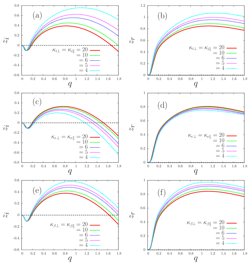
Figure 2: Imaginary part ($z_{i}$, left column) and real part ($z_{r}$, right column), of the normalized frequency for IC mode waves, vs. normalized wave number $q$, for different forms of ion and electron distribution functions, with several values of the kappa index. Parameters are $T_{i\perp}/T_{i\parallel}$= 5.0, $\epsilon=2.5\times 10^{-6}$, and other parameters as in figure 1. (a) and (b) PBK distribution with $\kappa_{i\perp}=\kappa_{i\parallel}$ for ions, with $\kappa$ values 20, 10, 6, 5, and 4, and Maxwellian distribution for electrons; (c) and (d) Bi-Maxwellian distribution for ions and PBK distribution for electrons, with $\kappa_{e\perp}=\kappa_{e\parallel}$, with $\kappa$ values 20, 10, 6, 5, and 4; (e) and (f) PBK distribution with $\kappa_{i\perp}=\kappa_{i\parallel}=5$ for ions and PBK distribution for electrons, with $\kappa_{e\perp}=\kappa_{e\parallel}$, and $\kappa$ values 20, 10, 6, 5, and 4.

In figure 2 we investigate the effect of the value of the kappa index on the EMIC instability, when ions and/or electrons are described by PBK distributions, considering fixed values of ion temperature ratio, $T_{i\perp}/T_{i\parallel}=5.0$, and dust relative number density, $\epsilon=2.5\times 10^{-6}$, with other parameters the same as those used in the case of figure 1. In figures 2(a) and 2(b) we show results obtained in the case that the electrons are described by a Maxwellian distribution, and the ions are described by a PBK distribution, considering five values of the kappa indexes, $\kappa_{i\perp}=\kappa_{i\parallel}=20$, 10, 6, 5, and 4. The ratios of effective temperatures are therefore $\theta_{i\perp}/\theta_{i\parallel}=5.14$, 5.31, 5.63, 5.83, and 6.25, respectively. Figure 2(a) shows that for $\kappa_{i}$ indexes equal to 20, the EMIC instability occurs for $0.2\leq q\leq 1.65$. With decrease of the kappa indexes to 10, the upper limit of the unstable region is moved to $q\simeq 1.8$, and the lower limit is decreased from the previous value. With further decrease of the kappa indexes, the unstable region increases considerably, extending well beyond the maximum value of $q$ which is shown in figure 1. The lower limit of the unstable region continues to decrease, being $q\simeq 0.13$ for kappa indexes equal to 4. The maximum value of the growth rate also increases with the decrease of the ion kappa indexes, being $z_{i}\simeq 0.38$ at $q\simeq 0.8$, in the case of $\kappa_{i\perp}=\kappa_{i\parallel}=20$, and $z_{i}\simeq 0.77$ at $q\simeq 1.1$, in the case of $\kappa_{i\perp}=\kappa_{i\parallel}=4$. For the real part of the dispersion relation, figure 2(b) shows that the effect of reduction of the kappa index in the ion distribution is and increase of the value of $z_{r}$, at all wavelengths.

In figure 2(c) and 2(d) we present results obtained from numerical solution of the dispersion relation in the case of ions described by a bi-Maxwellian distribution and electrons described by PBK distribution, with $\kappa_{e\perp}=\kappa_{e\parallel}=20$, 10, 6, 5, and 4. Despite the isotropy of electron temperature, $T_{e\perp}=T_{e\parallel}$, there is an effective electron anisotropy given by $\theta_{e\perp}/\theta_{e\parallel}$, which goes from 1.03 in the case of kappa indexes equal to 20, to 1.25 in the case of kappa indexes equal to 4. Figure 2(c) shows that the decrease of the kappa indexes of the electron distribution is associated to decrease in the magnitude of the growth rates and range of the EMIC instability, contrarily to what was observed in the case of decrease of the kappa indexes of the ion distribution, in figure 2(a). For the real part of the dispersion relation, figure 2(d) shows that the effect of the kappa index in the electron distribution is very small, much less significant than the effect due to the ion kappa indexes, seen in figure 2(b).

In figure 2(e) and 2(f) we depict results obtained considering both ions and electrons described by PBK distributions, with the same kappa indexes, considering kappa indexes 20, 10, 6, 5, and 4. In consonance with the results shown in figures 2(a) and 2(c), where it is seen that the growth rate of the EMIC instability tends to increase with the decrease of the kappa index in the ion PBK distribution, and decrease with the decrease of the kappa index in the electron PBK distribution, the results shown in figure 2(e) feature growth rates with values which are in between those obtained in panels (a) and (c). For instance, in the case of kappa values equal to 5, figure 2(e) shows that the maximum value of $z_{i}$ is nearly 0.51, while it is $z_{i}\simeq 0.6$ in the case of figure 2(a) and $z_{i}\simeq 0.23$ in figure 2(c).

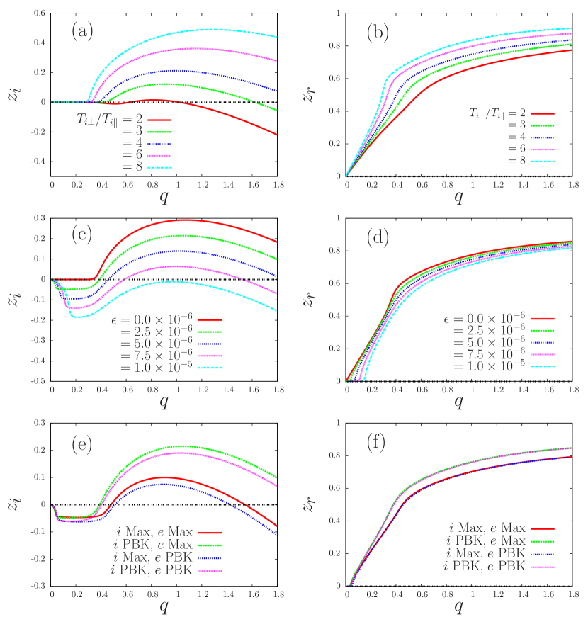
Figure 3: Imaginary part ($z_{i}$, left column) and real part ($z_{r}$, right column), of the normalized frequency for IC mode waves, vs. normalized wave number $q$. The plasma parameters are $\beta_{i}=0.2$, and other parameters as in figure 1. (a) and (b) PBK distribution for ions, with $\kappa_{i\perp}=\kappa_{i\parallel}=5.0$, and isotropic Maxwellian for electrons, and several values of the ion temperature ratio ($T_{i\perp}/T_{i\parallel}=2$, 3, 4, 6, and 8), in the absence of dust ($\epsilon=0$); (c) and (d) same combination of distribution functions as in panels (a) and (b), with $T_{i\perp}/T_{i\parallel}=5$, and different values of the dust density ratio ($\epsilon=0$, $2.5\times 10^{-6}$, $5.0\times 10^{-6}$, $7.5\times 10^{-6}$, and $1.0\times 10^{-5}$); (e) and (f) different combinations of ion and electron distribution functions, with $\epsilon=2.5\times 10^{-6}$ and $T_{i\perp}/T_{i\parallel}$= 5.0. PBK distributions are evaluated with $\kappa_{\beta\perp}=\kappa_{\beta\parallel}=5$.

Figure 3 reproduces the analysis made in figure 1, but considering $\beta_{i}=0.2$, instead of $\beta=2.0$. The comments which can be made about the results shown in figure 3(a) are qualitatively similar to those made about figure 1(a), with the difference that the onset of the instability in the case of lower $\beta_{i}$ occurs for larger values of $q$ than in the case of higher $\beta_{i}$, and that the instability in the case of lower $\beta_{i}$ requires slightly larger value of the ion temperature ratio in order to be started. Regarding the dependence on the dust density, figure 3(c) shows that the presence of dust leads to a reduction of the magnitude of the growth rates and in the range of unstable wave numbers, as in the case of higher $\beta_{i}$ presented in figure 1, with effectiveness which depends upon the velocity distribution functions. In the case of electrons with Maxwellian distribution and ions with PBK distribution with $\kappa_{i\perp}=\kappa_{i\parallel}=5.0$, shown in figures 3(c) and 3(d), the EMIC instability ceases to exist for $\epsilon\simeq 1.0\times 10^{-5}$. Panels (e) and (f) show the results of analysis of the effect of change in the particle distribution functions, for a given value of dust density ($\epsilon=2.5\times 10^{-6}$). It is seen in figure 3(e) that the use of a PBK ion distribution leads to significant increase in the magnitude of the growth rates and in the range of unstable wave numbers, similarly to what has been seen for higher $\beta_{i}$ in figure 1(e). Figure 3(e) also shows that the use of a PBK electron distribution leads to some decrease in the magnitude of the growth rate, but the effect is less pronounced than obtained in the case of figure 1(e). It is also seen in figure 3(e) that the damping region which appears for small $q$ is considerably larger than obtained in the case of higher $\beta_{i}$, in figure 1(e). Regarding the real part, the three panels in the right column of figure 3 show effects qualitatively similar to those shown in figure 1, but with less intense in the case of lower $\beta_{i}$ than in the case of higher $\beta_{i}$.

In figure 4 and 5 we investigate the effect of anisotropy of the $\kappa$ indexes in the ion distribution, considering isotropic electron and ion temperatures. The column at the left show the values of $z_{i}$, and the right column show the values of $z_{r}$.

In the case of figure 4, we consider a fixed value of the relative dust density, $\epsilon=2.5\times 10^{-6}$, and other parameters as in figure 1. For this figure, we assume PBK ion distributions, with isotropic temperatures, $\kappa_{i\parallel}=30$, and four values of $\kappa_{i\perp}$, namely $\kappa_{i\perp}=20$, 10, 5, and 2.93. These values of the ion kappa parameters correspond to effective ion temperature ratio given by 1.06, 1.19, 1.58, and 2.99, respectively. Panels (a) and (b) depict results obtained considering isotropic Maxwellian distribution for electrons, and panels (c) and (d)) show results obtained considering PBK distribution for electrons, with $\kappa_{e\perp}=\kappa_{e\parallel}=5.0$, and isotropic temperatures. We can compare the results appearing in figure 4(a) with those in figure 1(d), which was obtained considering the same parameters and similar combination of velocity distribution functions, except that in figure 1(d) the ion kappa indexes were isotropic and the ion temperatures were anisotropic. For instance, it is seen in figure 1(d) that for $T_{i\perp}/T_{i\parallel}=3.0$ there is instability in the range $0.2\leq q\leq 1.4$, with maximum value $z_{i}\simeq 0.25$. In the case of figure 4(a) the instability which appears for $\kappa_{i\perp}=2.93$ ($\theta_{i\perp}/\theta_{i\parallel}=2.99$) occurs for $0.3\leq q\leq 0.9$, with smaller value of the maximum growth rate. Another comparison which can be made is between the growth rates appearing in figures 4(c) and 1(h). Both figures show results obtained with PBK distributions for ions and electrons, with anisotropic temperatures in figure 1 and anisotropic ion kappa indexes in figure 4. In figure 1(h) the instability for $T_{i\perp}/T_{i\parallel}=3.0$ occurs in the region $0.22\leq q\leq 1.15$, with maximum growth rate which approaches $z_{i}=0.2$. In figure 4(c), the case with $\kappa_{i\perp}=2.93$, for which the ratio of effective temperature is $\theta_{i\perp}/\theta_{i\parallel}=2.99$, does not show positive values of $z_{i}$. The conclusion which can be drawn is that the anisotropy in the effective temperature which is due to the anisotropy of the kappa parameters of the ion distribution is not so effective as the anisotropy of the ion temperature parameters, on the effectiveness of the EMIC instability.

In figure 5 we investigate with more detail the role of the dust density in the case of ions with a PBK distribution, considering several values of the dust relative density, and other parameters which are the same as in the case of figure 1. Figures 5(a) and (b) show results obtained assuming a PBK ion distribution with isotropic temperatures and anisotropic kappa parameters, with an isotropic Maxwellian to describe the electron population. The ion kappa parameters are $\kappa_{i\parallel}=30$ and $\kappa_{i\perp}=2.93$, so that the effective temperature anisotropy of the ion distribution is $\theta_{i\perp}/\theta_{i\parallel}=2.99$. For this case, the values of $z_{i}$ seen in figure 5(a) show that the EMIC instability disappears for dust population between the values $\epsilon=2.5\times 10^{-6}$ and $\epsilon=5.0\times 10^{-6}$. Figures 5(c) and 5(d) show results obtained assuming that the electron distribution function is a PBK distribution, with isotropic temperatures and $\kappa_{e\parallel}=\kappa_{e\perp}=5.0$, instead of an isotropic Maxwellian, with the ion distribution and other parameters equal to those used in the case shown in figures 5(a) and 5(b). This example shows that, also in the case of ion distribution with anisotropy due to the kappa indexes, the increase of the non thermal character of the electron distribution, with the presence of a power-law electron tail, contributes to decrease the EMIC instability due to the anisotropic ion distribution.

For another comparison with the results shown in figure 5(a), figure 5(e) shows the values of $z_{i}$ obtained with isotropic Maxwellian distribution for electrons and PBK distribution for ions, with isotropic ion kappa indexes $\kappa_{i\perp}=\kappa_{i\parallel}=5.0$ and anisotropy due to the ion temperatures. We choose the ion temperature ratio as $T_{i\perp}/T_{i\parallel}=2.565$, which leads to the same anisotropy of the effective temperatures as in figure 5(a). It is seen that in the case of figure 5(e) the instability is slightly stronger, with larger range of unstable wave numbers, than in the case of figure 5(a). As already noticed in the commentaries about figure 4, it is seen that the anisotropy which is due to anisotropic ion kappa indexes is not so effective in producing the EMIC instability as the anisotropy due to the ion temperatures.

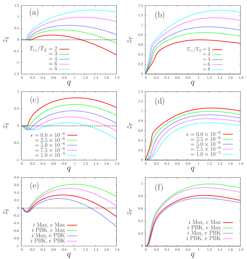
Figure 1: Imaginary part ($z_{i}$, left column) and real part ($z_{r}$, right column), of the normalized frequency for IC mode waves, vs. normalized wave number $q$. The plasma parameters are $\beta_{i}=2.0$, $v_{A}/c=1.0\times 10^{-4}$, $n_{i0}=1.0\times 10^{9}\,\mathrm{cm^{-3}}$, and $a=1.0\times 10^{-4}\,\mathrm{cm}$, with isotropic electron temperature, $T_{e}=T_{i\parallel}$. (a) and (b) PBK distribution for ions, with $\kappa_{i\perp}=\kappa_{i\parallel}=5.0$, and isotropic Maxwellian for electrons, and several values of the ion temperature ratio ($T_{i\perp}/T_{i\parallel}=2$, 3, 4, 6, and 8), in the absence of dust ($\epsilon=0$); (c) and (d) same combination of distribution functions as in panels (a) and (b), with $T_{i\perp}/T_{i\parallel}=5$, and different values of the dust density ratio ($\epsilon=0$, $2.5\times 10^{-6}$, $5.0\times 10^{-6}$, $7.5\times 10^{-6}$, and $1.0\times 10^{-5}$); (e) and (f) different combinations of ion and electron distribution functions, with $\epsilon=2.5\times 10^{-6}$ and $T_{i\perp}/T_{i\parallel}$= 5.0. PBK distributions are evaluated with $\kappa_{\beta\perp}=\kappa_{\beta\parallel}=5$.

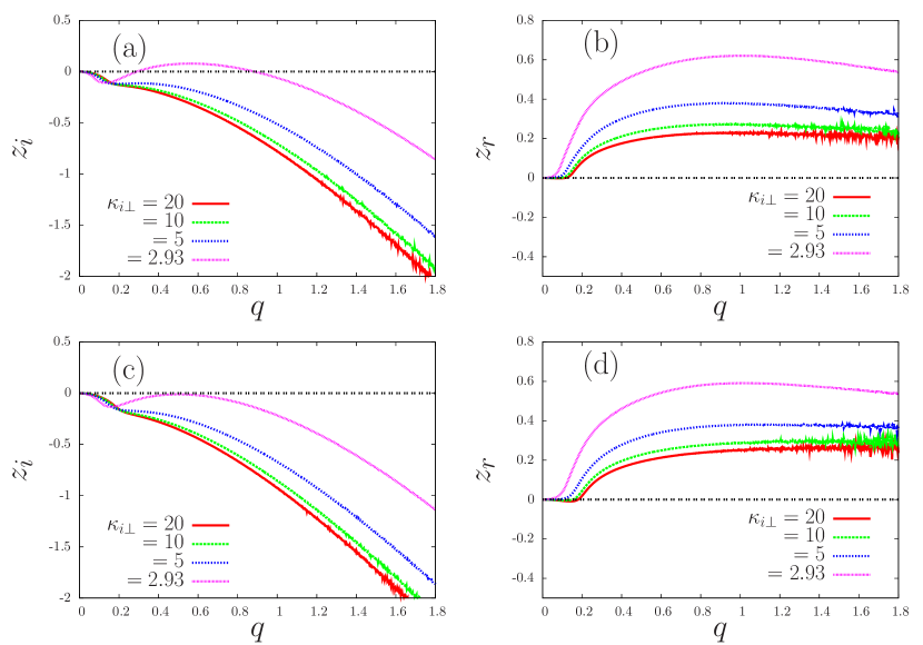
Figure 4: Imaginary part ($z_{i}$, left column) and real part ($z_{r}$, right column), of the normalized frequency for IC mode waves, vs. normalized wave number $q$, for different forms of ion and electron distribution functions, with isotropic ion temperatures and different values of anisotropy in the ion kappa indexes. Parameters are $\beta_{i}=2.0$, $v_{A}/c=1.0\times 10^{-4}$, $n_{i0}=1.0\times 10^{9}\,\mathrm{cm^{-3}}$, $a=1.0\times 10^{-4}\,\mathrm{cm}$, $\epsilon=2.5\times 10^{-6}$, and isotropic electron temperature $T_{e}=T_{i\parallel}$. (a) and (b) PBK distribution for ions, with $\kappa_{i\parallel}=30$ and several values of $\kappa_{i\perp}$ (20, 10, 5, and 2.93), and isotropic Maxwellian for electrons; (c) and (d) PBK distribution for ions, with $\kappa_{i\parallel}=30$ and several values of $\kappa_{i\perp}$ (20, 10, 5, and 2.93), and PBK distribution for electrons, with $\kappa_{e\parallel}=\kappa_{e\perp}=5.0$.

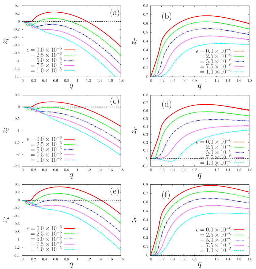
Figure 5: Imaginary part ($z_{i}$, left column) and real part ($z_{r}$, right column), of the normalized frequency for IC mode waves, vs. normalized wave number $q$, for different forms of ion and electron distribution functions, and several values of the relative dust number density ($\epsilon=0$, $2.5\times 10^{-6}$, $5.0\times 10^{-6}$, $7.5\times 10^{-6}$, and $1.0\times 10^{-5}$). Other parameters are $\beta_{i}=2.0$, $v_{A}/c=1.0\times 10^{-4}$, $n_{i0}=1.0\times 10^{9}\,\mathrm{cm^{-3}}$, $a=1.0\times 10^{-4}\,\mathrm{cm}$, and isotropic electron temperature $T_{e}=T_{i\parallel}$. (a) and (b) PBK distribution for ions, with $\kappa_{i\parallel}=30$ and $\kappa_{i\perp}=2.93$, with $T_{i\perp}=T_{i\parallel}$, and isotropic Maxwellian for electrons; (c) and (d) PBK distribution for ions, with $\kappa_{i\parallel}=30$ and $\kappa_{i\perp}=2.93$, with $T_{i\perp}=T_{i\parallel}$, and PBK distribution for electrons, with $\kappa_{e\parallel}=\kappa_{e\perp}=5.0$; (e) and (f) PBK distribution for ions, with $\kappa_{i\parallel}=\kappa_{i\perp}=5.0$ and $T_{i\perp}/T_{i\parallel}=2.565$, and isotropic Maxwellian for electrons.

4 Conclusions

We have presented results obtained from a numerical analysis of the dispersion relation for low-frequency ion-cyclotron waves propagating along the ambient magnetic field in a dusty plasma, considering situations where the velocity dispersion along perpendicular direction is greater than along the parallel direction, i.e., considering situations which can lead to the ion-cyclotron instability. It has been considered that either ions or electrons, or both, can have product-bi-kappa velocity distributions. Regarding the influence of the shape of the velocity distribution, results obtained considering absence of dust have shown that, if the electrons are described by an isotropic Maxwellian distribution and the ion distribution is changed from the bi-Maxwellian limit to a PBK distribution with relatively small kappa index, the range in wavenumber where instability occurs is increased, and the magnitude of the growth rates is increased as well. Conversely, if the ion distribution is a bi-Maxwellian distribution and the electron distribution is changed from a Maxwellian distribution into a PBK distribution with small kappa index, with isotropic electron temperature, the magnitude of the growth rates and range of the EMIC instability is somewhat reduced, but the magnitude of the reduction is less significant than the increase due to ion PBK distributions. Regarding the influence of dust, the results obtained have shown that, for all shapes of ion and electron distributions which have been utilized, the presence of a small population of dust leads to some decrease in the magnitude of the growth rates and in the range of the EMIC instability, in comparison with the case without dust. We have also seen that in presence of dust a region of wave damping appears for small values of $q$, which is not present in the dustless case. The appearing of this damping for large wavelengths, and the overall reduction in the growth rates of the instability in the presence of dust, are consequence of the collisional charging of the dust particles. All these features, related to different forms of ion and electron distributions and to the presence of a small amount of dust, have been obtained considering the plasma parameter $\beta_{i}=2.0$, and have also been verified considering one example with smaller value of this parameter, $\beta_{i}=0.2$.

Still regarding the effect of the presence of dust, the results obtained have shown that a value of the relative number density of dust which is enough to make disappear completely the EMIC instability in bi-Maxwellian plasma, may be not enough to overcome the instability in plasmas with ions described by PBK distributions with small kappa index. It has also been seen that the increase in the dust population leads to decrease of the phase velocity of the IC waves, for all types of combinations of Maxwellian and PBK distributions which have been investigated.

For fixed temperature ratio $T_{i\perp}/T_{i\parallel}$ and fixed dust number density, it has been seen that the decrease of the kappa index in a PBK ion distribution leads to increase of the instability in range and in magnitude of the growth rate, and that the increase becomes more and more pronounced for progressively smaller ion kappa indexes. On the other hand, for fixed value of $T_{i\perp}/T_{i\parallel}$ and dust density ratio, with bi-Maxwellian distribution for ions, the decrease of the kappa index in a PBK electron distribution leads to decrease of the EMIC instability, in magnitude of the growth rate and in range, but the decrease is not very pronounced. These features can be qualitatively explained as follows. For low frequency waves, the real parts of the arguments of the modified $Z$ function, which appear in the dispersion relation, are such that $|\zeta_{i}^{s}/\zeta_{e}^{s}|=\sqrt{(m_{i}/me)(T_{i\parallel}/T_{e\parallel})}$. In the case of bi-Maxwellian ion distribution and Maxwellian electron distribution, with $T_{i\parallel}=T_{e\parallel}$, it is known that the ion contribution is much more significant than the electron contribution, for the EMIC instability. For PBK ion distribution, the population of high energy ions is increased in comparison with the Maxwellian case, and can be compared to the high energy population of a higher temperature thermal plasma. Therefore, the instability growth rates of the EMIC are increased with the increase of the non thermal character of the PBK ion distribution. On the other hand, if the electrons are described by a PBK distribution, the population of resonant electrons may be much increased, in comparison with the thermal case. It is as if in the resonant region the ratio $|\zeta_{i}^{s}/\zeta_{e}^{s}|$ is decreased, by increase of an effective $T_{e\parallel}$. Therefore, electron cyclotron damping sets in, and the EMIC growth rates are reduced in comparison with the thermal case.

We have also investigated the effect of anisotropy in the kappa indexes of the ion PBK distribution, for given dust number density and for isotropic ion temperatures. It has been seen that the anisotropy due to the anisotropic kappa indexes is not so effective in producing the EMIC instability as the anisotropy due to the ratio between the ion perpendicular and parallel temperatures.

References

- Andre and Ferriere (2008) Andre, N., Ferriere, K.M.: J. Geophys. Res. 113(A9), 09202 (2008). doi:10.1029/2008JA013179
- Cattaert et al. (2007) Cattaert, T., Hellberg, M.A., Mace, R.L.: Physics Of Plasmas 14, 082111 (2007)
- Davidson and Ogden (1975) Davidson, R.C., Ogden, J.M.: Phys. Fluids 18(8), 1045 (1975). doi:10.1063/1.861253
-
de Juli et al. (2005)
de Juli, M.C.,
Schneider, R.S.,
Ziebell, L.F.,
Jatenco-Pereira, V.:
Phys. Plasmas
12(5),
052109
(2005).
doi:10.1063/1.1899647 -
de Juli et al. (2007)
de Juli, M.C.,
Schneider, R.S.,
Ziebell, L.F.,
Gaelzer, R.:
J. Geophys. Res.
112,
10105
(2007).
doi:10.1029/2007JA012434 - dos Santos et al. (2014) dos Santos, M.S., Ziebell, L.F., Gaelzer, R.: Phys. Plasmas 21, 112102 (2014). doi:10.1063/1.4900766
- dos Santos et al. (2015) dos Santos, M.S., Ziebell, L.F., Gaelzer, R.: Phys. Plasmas 22(12), 122107 (2015). doi:10.1063/1.4936972
- dos Santos et al. (2016) dos Santos, M.S., Ziebell, L.F., Gaelzer, R.: Phys. Plasmas 23(1), 013705 (2016). doi:10.1063/1.4939885
- Fried and Conte (1961) Fried, B.D., Conte, S.D.: The Plasma Dispersion Function. Academic Press, New York (1961)
- Galvão et al. (2011) Galvão, R.A., Ziebell, L.F., Gaelzer, R., de Juli, M.C.: Braz. J. Phys. 41(4-6), 258 (2011). doi:10.1007/s13538-011-0041-2
-
Gary et al. (1976)
Gary, S.P.,
Montgomery, M.D.,
Feldman, W.C.,
Forslund, D.W.:
J. Geophys. Res.
81(7),
1241
(1976).
doi:10.1029/JA081i007p01241 - Gary (2005) Gary, S.P.: Theory of Space Plasma Microinstabilities. Cambridge Atmospheric and Space Science Series. Cambridge, New York (2005)
-
Goertz (1989)
Goertz, C.K.:
Rev. Geophys.
27(2),
271
(1989).
doi:10.1029/RG027i002p00271 - Grün et al. (1985) Grün, E., Zook, H.A., Fechting, H., Giese, R.H.: Icarus 62(2), 244 (1985). doi:10.1016/0019-1035(85)90121-6
- Grün et al. (1997) Grün, E., Krüger, H., Dermott, S., Fectig, H., Graps, A.L., Zook, H.A., Gustafson, B.A., Hamilton, D.P., Hanner, M.S., Heck, A., Horányi, M., Kissel, J., Landblad, B.A., Linkert, D., Linkert, G., Mann, I., McDonnel, J.A.M., Morfill, G.E., Polanskey, C., Schwehm, G., Srama, R.: Geophys. Res. Lett. 24(17), 2171 (1997)
- Hapgood et al. (2011) Hapgood, M., Perry, C., Davies, J., Denton, M.: Planet. Space Sci. 59, 618 (2011). doi:10.1016/j.pss.2010.06.002
- Hellberg and Mace (2002) Hellberg, M., Mace, R.: Phys. Plasmas 9(5, 1), 1495 (2002). doi:10.1063/1.1462636
- Imai et al. (2015) Imai, M., Lecacheux, A., Moncuquet, M., Bagenal, F., Higgins, C.A., Imai, K., Thieman, J.R.: J. Geophys. Res. 120(3), 1888 (2015). doi:10.1002/2014JA020815
- Ishimoto and Mann (1998) Ishimoto, H., Mann, I.: Planet. Space Sci. 47(1-2), 225 (1998). doi:10.1016/0019-1035(85)90121-6
- Krueger et al. (2015) Krueger, H., Strub, P., Gruen, E., Sterken, V.J.: Astrophys. J 812(2), 139 (2015). doi:10.1088/0004-637X/812/2/139
- Kruger et al. (2007) Kruger, H., Landgraf, M., Altobelli, N., Grun, E.: Space Sci. Rev. 130(1-4), 401 (2007). doi:1016/j.asr.2007.04.066
-
Lazar (2012)
Lazar, M.:
Astron. Astrophys.
547,
94
(2012).
doi:10.1051/0004-6361/201219861 - Lazar and Poedts (2009a) Lazar, M., Poedts, S.: Astron. Astrophys. 494, 311 (2009a). doi:10.1051/0004-6361:200811109
- Lazar and Poedts (2009b) Lazar, M., Poedts, S.: Solar Phys. 258, 119 (2009b). doi:10.1007/s11207-009-9405-y
- Lazar and Poedts (2014) Lazar, M., Poedts, S.: Mon. Not. R. Astron. Soc. 437(1), 641 (2014). doi:10.1093/mnras/stt1914
- Lazar et al. (2015) Lazar, M., Poedts, S., Fichtner, H.: Astron. Astrophys. 582, 124 (2015). doi:10.1051/0004-6361/201526509
- Lazar et al. (2011) Lazar, M., Poedts, S., Schlickeiser, R.: Astron. Astrophys. 534, 116 (2011). doi:10.1051/0004-6361/201116982
- Lazar et al. (2010) Lazar, M., Schlickeiser, R., Poedts, S.: Phys. Plasmas 17, 062112 (2010). doi:10.1063/1.3446827
- Lazar et al. (2012) Lazar, M., Pierrard, V., Poedts, S., Schlickeiser, R.: Astrophys. Space Sci. Proc. 33, 97 (2012)
- Leubner (2002) Leubner, M.P.: Astrophys. Space Sci. 282(3), 573 (2002). doi:10.1023/A:1020990413487
- Livadiotis and McComas (2013a) Livadiotis, G., McComas, D.J.: Space Sci. Rev. 175, 215 (2013a). doi:10.1007/s11214-013-9996-3
- Livadiotis and McComas (2013b) Livadiotis, G., McComas, D.J.: Space Sci. Rev. 175, 183 (2013b). doi:10.1007/s11214-013-9982-9
- Livadiotis (2015) Livadiotis, G.: J. Geophys. Res. 120(3), 1607 (2015). doi:10.1002/2014JA020825
- Maksimovic et al. (1997) Maksimovic, M., Pierrard, V., Lemaire, J.F.: Astron. Astrophys. 324(2), 725 (1997)
- Maksimovic et al. (2005) Maksimovic, M., Zouganelis, I., Chaufray, J.-Y., Issautier, K., Scime, E.E., Littleton, J.E., Marsch, E., McComas, D.J., Salem, C., Lin, R.P., Elliot, H.: J. Geophys. Res. 110, 09104 (2005). doi:10.1029/2005JA011119
-
Mann (2008)
Mann, I.:
Adv. Space Res.
41(1),
160
(2008).
doi:1016/j.asr.2007.04.066 -
Mann et al. (2004)
Mann, I.,
Kimura, H.,
Biesecker, D.A.,
Tsurutani, B.T.,
Grun, E.,
McKibben, R.B.,
Liou, J.C.,
MacQueen, R.M.,
Mukai, T.,
Guhathakurta, M.,
Lamy, P.:
Space Sci. Rev.
110(3-4),
269
(2004).
doi:10.1023/B:SPAC.0000023440.82735.ba - Mann (2010) Mann, I.: Annu. Rev. Astron. Astrophys. 48, 173 (2010). doi:10.1146/annurev-astro-081309-130846
- Marsch et al. (2004) Marsch, E., Ao, X.-Z., Tu, C.-Y.: J. Geophys. Res. 109, 04102 (2004). doi:10.1029/2003JA010330
- Marsch (2006) Marsch, E.: Living Rev. Solar Phys. 3(1), 1 (2006). cited 19 Sep. 2006, http://www.livingreviews.org/lrsp-2006-1. doi:10.12942/lrsp-2006-1
- Mendis and Horányi (2013) Mendis, D.A., Horányi, M.: Rev. Geophys. 51(1), 53 (2013). doi:10.1002/rog.20005
- Meyer-Vernet et al. (2009) Meyer-Vernet, N., Maksimovic, M., Czechowski, A., Mann, I., Zouganelis, I., Goetz, K., Kaiser, M.L., Cyr, O.C.S., Bougeret, J.-L., Bale, S.D.: Solar Phys. 256(1), 463 (2009). doi:10.1007/s11207-009-9349-2
- Moncuquet et al. (2002) Moncuquet, M., Bagenal, F., Meyer-Vernet, N.: J. Geophys. Res. 107(A9), 1260 (2002). doi:10.1029/2001JA900124
- Pierrard and Lazar (2010) Pierrard, V., Lazar, M.: Solar Phys. 267(1), 153 (2010). doi:10.1007/s11207-010-9640-2
- Pilipp et al. (1987a) Pilipp, W., Miggenrieder, H., Montgomery, M., Mühlhäuser, K.-H., Rosenbauer, H., Schwenn, R.: J. Geophys. Res. 92(A2), 1075 (1987a). doi:10.1029/JA092iA02p01075
- Pilipp et al. (1987b) Pilipp, W., Miggenrieder, H., Montgomery, M., Mühlhäuser, K.-H., Rosenbauer, H., Schwenn, R.: J. Geophys. Res. 92(A2), 1093 (1987b). doi:10.1029/JA092iA02p01093
- Rao (1993) Rao, N.N.: Phys. Scr. 48(3), 363 (1993). doi:10.1088/0031-8949/48/3/015
-
Schneider et al. (2006)
Schneider, R.S.,
Ziebell, L.F.,
de Juli, M.C.,
Jatenco-Pereira, V.:
Braz. J. Phys.
36(3A),
759
(2006).
doi:10.1590/S0103-97332006000500033 -
Schwenn (2006)
Schwenn, R.:
Space Sci. Rev.
124,
51
(2006).
doi:10.1007/s11214-006-9099-5 - Shukla (1992) Shukla, P.K.: Phys. Scr. 45, 504 (1992). doi:10.1088/0031-8949/45/5/014
- Summers and Thorne (1991) Summers, D., Thorne, R.M.: Phys. Fluids B 3(8), 1835 (1991). doi:10.1063/1.859653
- Tsytovich et al. (2002) Tsytovich, V.N., de Angelis, U., Bingham, R.: Phys. Plasmas 9(4), 1079 (2002)
- Tsytovich et al. (2004) Tsytovich, V.N., Morfill, G.E., Thomas, H.: Plasma Phys. Rep. 30(10), 816 (2004). doi:10.1134/1.1809401
- Vasyliunas (1968) Vasyliunas, V.M.: J. Geophys. Res. 73(9), 2839 (1968). doi:10.1029/JA073i009p02839
- Ziebell et al. (2008) Ziebell, L.F., Schneider, R.S., de Juli, M.C., Gaelzer, R.: Braz. J. Phys. 38(3A), 297 (2008). doi:10.1590/S0103-97332008000300002