Sharp magnetic structures from dynamos with density stratification

Abstract

Recent direct numerical simulations (DNS) of large-scale turbulent dynamos in strongly stratified layers have resulted in surprisingly sharp bipolar structures at the surface. Here we present new DNS of helically and non-helically forced turbulence with and without rotation and compare with corresponding mean-field simulations (MFS) to show that these structures are a generic outcome of a broader class of dynamos in density-stratified layers. The MFS agree qualitatively with the DNS, but the period of oscillations tends to be longer in the DNS. In both DNS and MFS, the sharp structures are produced by converging flows at the surface and might be driven in nonlinear stage of evolution by the Lorentz force associated with the large-scale dynamo-driven magnetic field if the dynamo number is at least 2.5 times supercritical.

1 Introduction

Active regions appear at the solar surface as bipolar patches with a sharply defined polarity inversion line in between. Bipolar magnetic structures are generally associated with buoyant magnetic flux tubes that are believed to pierce the surface (Parker, 1955). Furthermore, Parker (1975) proposed that only near the bottom of the convection zone the large-scale field can evade magnetic buoyancy losses over time scales comparable with the length of the solar cycle. This led many authors to study the evolution of magnetic flux tubes rising from deep within the convection zone to the surface (Caligari et al., 1995; Fan, 2001, 2008; Jouve & Brun, 2009). Shortly before flux emergence, however, the rising flux tube scenario would predict flow speeds that exceed helioseismically observed limits (Birch et al., 2016). Moreover, the magnetic field expands and weakens significantly during its buoyant ascent. Therefore, some type of reamplification of magnetic field structures near the surface appears to be necessary.

The negative effective magnetic pressure instability (NEMPI) may be one such mechanism of field reamplification. It has been intensively studied both analytically (Kleeorin et al., 1989, 1990, 1993, 1996; Kleeorin & Rogachevskii, 1994; Rogachevskii & Kleeorin, 2007) and numerically using direct numerical simulations (DNS) and mean-field simulations (MFS) (Brandenburg et al., 2010, 2011, 2012, 2013, 2014), see also the recent review by Brandenburg et al. (2016). The reamplification mechanism of magnetic structures in DNS has been studied in non-helical forced turbulence (Brandenburg et al., 2011, 2013, 2014; Warnecke et al., 2013, 2016) and in turbulent convection (Käpylä et al., 2012, 2016) with imposed weak horizontal or vertical magnetic fields. However, NEMPI seems to work only when the magnetic field is not too strong (magnetic energy density is less than the turbulent kinetic energy density).

The formation of magnetic structures from a dynamo-generated field has recently been studied for forced turbulence (Mitra et al., 2014; Jabbari et al., 2014, 2015, 2016) and in turbulent convection (Masada & Sano, 2016). In particular, simulations by Mitra et al. (2014) have shown that much stronger magnetic structures can occur at the surface when the field is generated by a large-scale $\alpha^{2}$ dynamo in forced helical turbulence. Subsequent work by Jabbari et al. (2016) suggests that bipolar surface structures are kept strongly concentrated by converging flow patterns which, in turn, are produced by a strong magnetic field through the Lorentz force. This raises the question what kind of nonlinear interactions take place when a turbulent dynamo operates in a density-stratified layer. To investigate this problem in more detail, we study here the dynamics of magnetic structures both in DNS and MFS in similar parameter regimes.

The original work of Mitra et al. (2014) employed a two-layer system, where the turbulence is helical only in the lower part of the system, while in the upper part it is nonhelical. Such two-layer forced turbulence was also studied in spherical geometry (Jabbari et al., 2015). They showed that in such a case, several bipolar structures form, which later expand and create a band-like arrangement. The two-layer system allowed us to separate the dynamo effect in the lower layer from the effect of formation of intense bipolar structures in the upper layer. The formation of flux concentrations from a dynamo-generated magnetic field in spherical geometry was also investigated with MFS (Jabbari et al., 2013). In that paper, NEMPI was considered as the mechanism creating flux concentrations. Models similar to those of Mitra et al. (2014) have also been studied by Jabbari et al. (2016), who showed that a two-layer setup is not necessary and that even a single layer with helical forcing leads to formation of intense bipolar structures. This simplifies matters, and such systems will therefore be studied here in more detail before addressing associated MFS of corresponding $\alpha^{2}$ dynamos. In earlier work of Mitra et al. (2014) and Jabbari et al. (2016), no conclusive explanation for the occurrence of bipolar structures with a sharp boundary was presented.

We use both DNS and MFS to understand the mechanism behind the nonlinear interactions resulting in the complex dynamics of sharp bipolar spots. One of the key features of such dynamics is the long lifetime of the sharp bipolar spots that tend to persist several turbulent diffusion times. It has been shown by Jabbari et al. (2016) that the long-term existence of these sharp magnetic structures is accompanied by the phenomenon of turbulent magnetic reconnection in the vicinity of current sheets between opposite magnetic polarities. The measured reconnection rate was found to be nearly independent of magnetic diffusivity and Lundquist number.

In this work, we study the formation and dynamics of sharp magnetic structures both in one-layer DNS and in corresponding MFS. We begin by discussing the model and the underlying equations both for the DNS and the MFS (Sect. 2), and then present the results (Sect. 3), where we focus on the comparison between DNS and MFS. In the DNS, the dynamo is driven either directly by helically forced turbulence or indirectly by nonhelically forced turbulence that becomes helical through the combined effects of stratification and rotation, as will be discussed at the end of Sect. 3. We conclude in Sect. 4.

2 The model

We perform simulations in Cartesian coordinates following Jabbari et al. (2016). In our DNS, we study a one-layer model in which the forcing is helical in the entire domain. In the following we describe the details of both DNS and MFS.

2.1 DNS equations

First, we study an isothermally stratified layer in DNS and solve the magnetohydrodynamic equations for the velocity $U$, the magnetic vector potential $A$, and the density $\rho$ in the presence of rotation $\Omega$,

$${\partial\rho\over\partial t}=-\mbox{\boldmath$\nabla$}{}\cdot\rho\mbox{\boldmath$U$}{},$$ (1)

$$\rho{{\rm D}{}\mbox{\boldmath$U$}{}\over{\rm D}{}t}=\mbox{\boldmath$J$}{}\times\bm{B}-c_{\rm s}^{2}\mbox{\boldmath$\nabla$}{}\rho-2\bm{\Omega}\times\rho\mbox{\boldmath$U$}{}+\rho(\mbox{\boldmath$f$}{}+\mbox{\boldmath$g$}{})+\mbox{\boldmath$\nabla$}{}\cdot(2\nu\rho\mbox{\boldmath${\sf S}$}{}),\;\;$$ (2)

$${\partial\mbox{\boldmath$A$}{}\over\partial t}=\mbox{\boldmath$U$}{}\times\bm{B}+\eta\nabla^{2}\mbox{\boldmath$A$}{},$$ (3)

where the operator ${\rm D}{}/{\rm D}{}t=\partial/\partial t+\mbox{\boldmath$U$}{}\cdot\mbox{\boldmath$\nabla$}{}$ is the advective derivative, $\bm{\Omega}=(-\sin\theta,0,\cos\theta)\Omega$ is the angular velocity with $\theta$ being colatitude, $\eta$ is the magnetic diffusivity, $\mbox{\boldmath$g$}{}=(0,0,-g)$ is the gravitational acceleration, $\bm{B}=\mbox{\boldmath$\nabla$}{}\times\mbox{\boldmath$A$}{}$ is the magnetic field, $\mbox{\boldmath$J$}{}=\mbox{\boldmath$\nabla$}{}\times\bm{B}/\mu_{0}$ is the current density, ${\sf S}_{ij}={\textstyle{1\over 2}}(U_{i,j}+U_{j,i})-{\textstyle{1\over 3}}\delta_{ij}\mbox{\boldmath$\nabla$}{}\cdot\mbox{\boldmath$U$}{}$ is the traceless rate of strain tensor (the commas denote partial differentiation), $\nu$ is the kinematic viscosity, $c_{\rm s}$ is the isothermal sound speed, and $\mu_{0}$ is the vacuum permeability. We adopt Cartesian coordinates $(x,y,z)$ and perform isothermal simulations, so there is no possibility of convection. Turbulence is produced by the forcing function $f$ that consists of random, white-in-time, plane waves with a certain average wavenumber $k_{\rm f}$ (Brandenburg, 2001; Mitra et al., 2014):

$$\mbox{\boldmath$f$}{}(\bm{x},t)={\rm Re}\{N\tilde{{\bm{f}}}(\bm{k},t)\exp[{\rm i}\bm{k}\cdot\bm{x}+{\rm i}\phi]\},$$ (4)

where $\bm{x}$ is the position vector. We choose $N=f_{0}\sqrt{c_{\rm s}^{3}|\bm{k}|}$, where $f_{0}$ is a nondimensional forcing amplitude. At each timestep, we select randomly the phase $-\pi<\phi\leq\pi$ and the wavevector $\bm{k}$ from many possible discrete wavevectors in a certain range around a given forcing wavenumber, $k_{\rm f}$. Hence $\mbox{\boldmath$f$}{}(t)$ is a stochastic process that is white-in-time and is integrated by using the Euler–Maruyama scheme (Higham, 2001). The Fourier amplitudes,

$$\tilde{{\bm{f}}}({\bm{k}})=\mbox{\boldmath${\sf R}$}{}\cdot\tilde{{\bm{f}}}({\bm{k}})^{\rm(nohel)}\quad\mbox{with}\quad{\sf R}_{ij}={\delta_{ij}-{\rm i}\sigma\epsilon_{ijk}\hat{k}\over\sqrt{1+\sigma^{2}}},$$ (5)

where the parameter $\sigma$ characterizes the fractional helicity of $f$, and

$$\tilde{{\bm{f}}}({\bm{k}})^{\rm(nohel)}=\left(\bm{k}\times\hat{\mbox{\boldmath$e$}}{}\right)/\sqrt{\bm{k}^{2}-(\bm{k}\cdot\hat{\mbox{\boldmath$e$}}{})^{2}}$$ (6)

is a non-helical forcing function. Here $\hat{\mbox{\boldmath$e$}}{}$ is an arbitrary unit vector not aligned with $\bm{k}$, $\hat{\bm{k}}$ is the unit vecntor along $\bm{k}$, and $|\tilde{{\bm{f}}}|^{2}=1$ (Brandenburg, 2001). In most of the simulations, $f$ is maximally helical with positive helicity, but we also consider cases without helicity. The turbulent rms velocity is approximately independent of $z$ with $u_{\rm rms}=\langle\mbox{\boldmath$u$}{}^{2}\rangle^{1/2}\approx 0.1\,c_{\rm s}$.

We consider a cubic domain of size $L^{3}$ with $-L/2\leq x,y,z\leq L/2$ and define the base wavenumber as $k_{1}=2\pi/L$. The density scale height is $H_{\rho}=c_{\rm s}^{2}/g$, where the value of $g$ is chosen such that $k_{1}H_{\rho}=1$, so the density contrast between top and bottom is $\exp(2\pi)\approx 535$. In the following, we refer to $k_{\rm f}/k_{1}$ as the scale separation ratio.

2.2 MFS equations

For the MFS, we consider the nonrotating case of a conducting isothermal gas governed by the equations for the mean density $\overline{\rho}$, the mean (large-scale) velocity $\overline{\mbox{\boldmath$U$}}{}$, the mean vector potential $\overline{\mbox{\boldmath$A$}}{}$, so that the mean magnetic field is given by $\overline{\mbox{\boldmath$B$}}{}=\mbox{\boldmath$\nabla$}{}\times\overline{\mbox{\boldmath$A$}}{}$. Thus,

$${\partial\overline{\rho}\over\partial t}=-\mbox{\boldmath$\nabla$}{}\cdot\overline{\rho}\overline{\mbox{\boldmath$U$}}{},$$ (7)

$$\overline{\rho}{\overline{D}\,\overline{\mbox{\boldmath$U$}}{}\over{\rm D}{}t}=\overline{\mbox{\boldmath$J$}}{}\times\overline{\mbox{\boldmath$B$}}{}-c_{\rm s}^{2}\mbox{\boldmath$\nabla$}{}\overline{\rho}+\overline{\rho}\mbox{\boldmath$g$}{}+\mbox{\boldmath$\nabla$}{}\cdot(2\nu_{\rm T}\overline{\rho}\overline{\mbox{\boldmath${\mathsf{S}}$}}{}),$$ (8)

$${\partial\overline{\mbox{\boldmath$A$}}{}\over\partial t}=\overline{\mbox{\boldmath$U$}}{}\times\overline{\mbox{\boldmath$B$}}{}+\alpha\overline{\mbox{\boldmath$B$}}{}+\eta_{\rm T}\nabla^{2}\overline{\mbox{\boldmath$A$}}{},$$ (9)

where $\alpha$ is given by (Iroshnikov, 1971)

$$\alpha={\alpha_{0}\over 1+Q_{\alpha}\overline{\mbox{\boldmath$B$}}{}^{2}/B_{\rm eq}^{2}},$$ (10)

and $\overline{D}/{\rm D}{}t=\partial/\partial t+\overline{\mbox{\boldmath$U$}}{}\cdot\mbox{\boldmath$\nabla$}{}$ is the advective derivative with respect to the mean flow, $\eta_{\rm T}$ and $\nu_{\rm T}$ are the total (sums of turbulent and microphysical) magnetic diffusivity and kinematic viscosity, respectively, $\alpha_{0}$ quantifies the kinematic $\alpha$ effect, $Q_{\alpha}$ determines the strength of the $\alpha$ quenching, $\overline{\mbox{\boldmath$J$}}{}=\mbox{\boldmath$\nabla$}{}\times\overline{\mbox{\boldmath$B$}}{}/\mu_{0}$ is the mean current density, $\overline{\mbox{\boldmath${\mathsf{S}}$}}{}$ is the traceless rate of strain tensor of the mean flow with components $\overline{\mathsf{S}}_{ij}={\textstyle{1\over 2}}(\overline{U}_{i,j}+\overline{U}_{j,i})-{\textstyle{1\over 3}}\delta_{ij}\mbox{\boldmath$\nabla$}{}\cdot\overline{\mbox{\boldmath$U$}}{}$, and $B_{\rm eq}=\sqrt{\mu_{0}\rho}\,u_{\rm rms}$ is the equipartition field strength.

2.3 Boundary and initial conditions

We adopt periodic boundary conditions in the $x$ and $y$ directions and stress-free conditions at top and bottom ($z=\pm L/2$). The magnetic field boundary conditions are perfect conductor at the bottom and vertical field at the top.

In the MFS, we perform two-dimensional and three-dimensional simulations. For the two-dimensional MFS we adopt a squared-shaped Cartesian domain of size $L^{2}$ in the $x$ and $z$ directions, respectively. Periodic boundary conditions are applied in the $x$ and $y$ directions and perfectly conducting boundaries for the magnetic field at the bottom ($z=-L/2$),

$$A_{x}=A_{y}=A_{z,z}=0\quad\mbox{at $z=-L/2$ (bottom)},$$ (11)

and vertical field conditions at the top ($z=L/2$)

$$A_{x,z}=A_{y,z}=A_{z}=0\quad\mbox{at $z=L/2$ (top)}.$$ (12)

For the velocity field, both boundaries are assumed stress-free, i.e.,

$$U_{x,z}=U_{y,z}=U_{z}=0\quad\mbox{at $z=\pm L/2$}.$$ (13)

The same conditions apply to the MFS, but with $\mbox{\boldmath$A$}{}\to\overline{\mbox{\boldmath$A$}}{}$ and $\mbox{\boldmath$U$}{}\to\overline{\mbox{\boldmath$U$}}{}$. As initial conditions we adopt a hydrostatic equilibrium with $\rho=\rho_{0}\exp(-z/H_{\rho})$, where $\rho_{0}$ is a constant. The initial magnetic field consists of weak gaussian-distributed noise.

2.4 Parameters of the simulations

Our units are chosen such that $c_{\rm s}=g=\mu_{0}=1$. In most of the calculations, we use $k_{\rm f}/k_{1}=30$, except in one case where we decrease it to $5$ to study the effect of changing the scale separation ratio. For the reference run, we use a Reynolds number $\mbox{\rm Re}\equiv u_{\rm rms}/\nu k_{\rm f}$ of 100, and a magnetic Prandtl number $\mbox{\rm Pr}_{M}=\nu/\eta$ of 0.5. The magnetic Reynolds number, $\mbox{\rm Re}_{M}\equiv u_{\rm rms}/\eta k_{\rm f}$, is therefore $\mbox{\rm Re}_{M}=\mbox{\rm Pr}_{M}\mbox{\rm Re}=50$.

Following earlier work by Brandenburg et al. (2009), a more natural length scale is given by the inverse wavenumber of the most slowly decaying mode, which corresponds to a quarter wave and is given by

$$\tilde{k}_{1}=\pi/2L.$$ (14)

With the boundary conditions (11) and (12), the most easily excited solution corresponds to dynamo waves propagating in the positive $z$ direction, as was found by Brandenburg et al. (2009). As in earlier work, a relevant timescale is the turbulent-diffusive time given by

$$\tau_{\rm td}=(\eta_{\rm T}\tilde{k}_{1}^{2})^{-1}.$$ (15)

When comparing with earlier work of Mitra et al. (2014) and Jabbari et al. (2016), we must remember that they defined the turbulent-diffusive time $\tau_{\rm td}^{\prime}=\tau_{\rm td}/16$ based on $k_{1}$.

The system is characterized by the following set of non-dimensional numbers: the dynamo number and an analogous number characterizing $u_{\rm rms}$, i.e.,

$$C_{\alpha}=\alpha_{0}/\eta_{\rm T}\tilde{k}_{1},\quad C_{u}=u_{\rm rms}/\eta_{\rm T}\tilde{k}_{1},$$ (16)

as well as the turbulent magnetic Prandtl number and the Froude number,

$$\mbox{\rm Pr}_{M}^{\rm turb}=\nu_{\rm T}/\eta_{\rm T},\quad\mbox{\rm Fr}=u_{\rm rms}\,\sqrt{\tilde{k}_{1}/g},$$ (17)

respectively. In the MFS, it enters only indirectly through the definition of $B_{\rm eq}$. The value of $B_{\rm eq}$ in the middle of the domain is $B_{\rm eq0}=B_{\rm eq}(z=0)$. For the DNS of rotating turbulence, we also define the Coriolis number,

$$\mbox{\rm Co}=2\Omega/u_{\rm rms}k_{\rm f}.$$ (18)

All calculations have been performed with the Pencil Code. It uses sixth-order explicit finite differences in space and a third-order accurate time-stepping method. In the DNS, we adopt a numerical resolution of $256\times 252\times 256$ mesh points in the $x$, $y$, and $z$ directions in the Cartesian coordinate. In the two- and three-dimensional MFS, we used $288^{2}$ or $288^{3}$ meshpoints, respectively.

2.5 Simulation strategy

As alluded to in the introduction, we want to study here a model that is as simple as possible. Before addressing the MFS, let us first consider the DNS. The simpler one-layer model was already studied by Jabbari et al. (2016); see their Run RM1zs. In the following we focus on particular properties that are relevant for our comparison with related MFS.

In the present work, we investigate the behavior of an $\alpha^{2}$ dynamo and the formation of the structures with sharp boundaries. We perform systematic parameter studies similar to Jabbari et al. (2016) to investigate the effect of changing magnetic Reynolds number and scale separation on the structures. Furthermore, in some runs we include the Coriolis force in the momentum equation to study the influence of rotation in our model.

Table 1: Summary of the DNS with helical forcing. The reference run is shown in bold.

Run $\mbox{\rm Re}_{M}$ $k_{\rm f}/k_{1}\!\!\!\!$ Co $\;\;\tilde{\lambda}$ R1 50 30 0 0.013 R2 130 30 0 0.002 R3 260 30 0 0.001 R4 50 5 0 0.028 R5 50 30 0.3 0.01 R6 50 30 0.7 0.009 R7 50 30 1.4 0.005

3 Results

In the following we start with DNS of helically forced turbulence, compare with corresponding MFS, and finally study DNS with nonhelically forced rotating turbulence. In the latter case, the presence of rotation together with the density stratification produce helicity and thus large-scale dynamo action.

3.1 The one-layer model in DNS

We begin with the helically forced case. The parameters of our DNS with helically forced turbulence are summarized in Table LABEL:Tab1. Here we also give a nondimensional estimate of the dynamo growth rate, $\tilde{\lambda}=\lambda/u_{\rm rms}k_{\rm f}$, where $\lambda={\rm d}{}\ln B_{\rm rms}/{\rm d}{}t$ is the instantaneous growth rate. One can see that its value decreases with increasing magnetic Reynolds number and with faster rotation, which is consistent with the results of Jabbari et al. (2016); see their Fig. 2 and the discussion in their Section 3.

3.1.1 Structure of the large-scale field

The dynamo-generated magnetic field is time-dependent. This is caused by an underlying oscillatory $\alpha^{2}$-type dynamo mechanism that has been seen in earlier DNS (Mitra et al., 2010; Warnecke et al., 2011). It leads to a migratory dynamo wave from the lower perfect conductor boundary toward the upper vacuum boundary (Brandenburg et al., 2009; Brandenburg, 2017). Although the mean magnetic field of this dynamo has no $z$ component, it develops one in the nonlinear stage, albeit with zero net vertical flux. During certain times, the associated horizontal field locks into a state where it is aligned with one of the two horizontal coordinate directions. This alignment is a consequence of having adopted a horizontally periodic domain. In Run R1, it points in the $x$ direction during the time shown in Fig. 1, where we have selected an arbitrarily chosen cross-section of $B_{x}$ in the $yz$ plane. Clearly, the field is strongest in the deeper parts, $z/H_{\rho}\approx-2$, and varies only little in the upper parts, $-1\leq z/H_{\rho}\leq\pi$. By contrast, the vertical field $B_{z}$ is strongest in the upper parts, $1\leq z/H_{\rho}\leq\pi$ (see Fig. 2), and develops sharp structures that are clearly seen at the top surface. In particular, we see the formation of a sharp structure associated with a Y-point current sheet structure, similarly to that was shown in Figure 9 of Jabbari et al. (2016), where the associated reconnection phenomenology was studied in detail. The resulting surface structure is shown in Fig. 3, where the formation of a current sheet and subsequent reconnection of the magnetic field lines occur in the time interval between $t/\tau_{\rm td}=2.4$ and $2.7$.

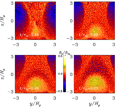
Figure 1: DNS for $\mbox{\rm Re}_{M}=50$ (Run R1). Time evolution of $B_{x}/B_{\rm eq}$ in the $yz$ plane through $x/H_{\rho}=\pi$.

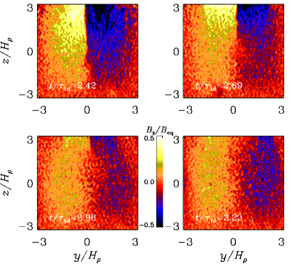
Figure 2: DNS for $\mbox{\rm Re}_{M}=50$ (Run R1): time evolution of $B_{z}/B_{\rm eq}$ in the $yz$ plane through $x/H_{\rho}=\pi$.

3.1.2 Growth and evolution of the magnetic field

In all of our simulations, the initial magnetic field grows rapidly to become comparable to $B_{\rm eq}$, so no clear kinematic dynamo stage can be seen. This has the advantage that these simulations reach quickly a nonlinear statistically steady state. On the other hand, for such strong magnetic fields NEMPI cannot be observed in DNS. Similar to our earlier work, we find that, in the nonlinear stage, the amplitudes of the oscillations of the kinetic and magnetic energy densities are small; see Fig. 4.

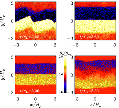
Figure 3: DNS for $\mbox{\rm Re}_{M}=50$: time evolution of $B_{z}/B_{\rm eq}$ in the $xy$ plane through $z/H_{\rho}=\pi$ for Run R1.

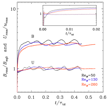
Figure 4: DNS for $\mbox{\rm Re}_{M}=50,130,260$: $B_{\rm rms}/B_{\rm eq0}$ (solid) and $U_{\rm rms}/u_{\rm rms}$ (dashed) versus time. Different colors represent different values of $\mbox{\rm Re}_{M}$: 50 for Run R1 (black), 130 for Run R2 (blue), and 260 for Run R3 (red). The inset shows the early times.

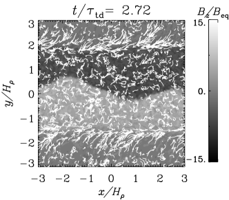
Figure 5: Velocity vectors $(U_{x},U_{y})$ at the surface ($z/H_{\rho}=\pi$) for Run R1 (DNS for $\mbox{\rm Re}_{M}=50$) superimposed on a gray-scale representation of $B_{z}/B_{\rm eq}(z)$ at $t/\tau_{\rm td}=2.46$.

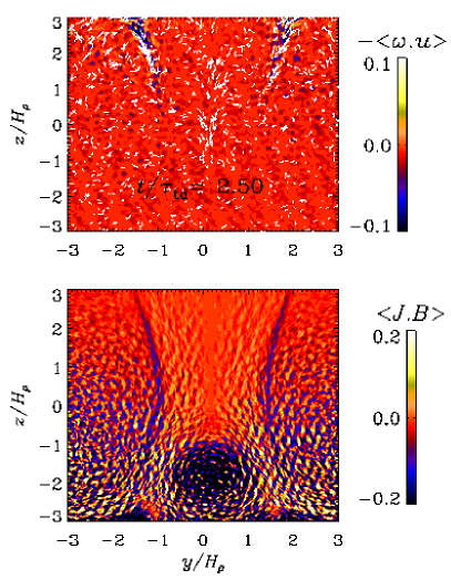
Figure 6: DNS for $\mbox{\rm Re}_{M}=50$ (Run R1): negative mean kinetic and positive current helicity densities averaged along the $x$ direction.

3.1.3 Horizontal flows along magnetic boundaries

We tend to find systematic horizontal flows along magnetic boundaries. This is demonstrated in Fig. 5, where we show horizontal flow vectors together with a gray-scale representation of the magnetic field. These horizontal flows are in opposite directions on both sides. If those horizontal flows are associated with systematic vertical flows, they would imply a systematic helicity. In Fig. 6 we plot the mean kinetic helicity, $\langle\mbox{\boldmath$\omega$}{}\cdot\mbox{\boldmath$u$}{}\rangle$, where $\mbox{\boldmath$\omega$}{}=\mbox{\boldmath$\nabla$}{}\times\mbox{\boldmath$u$}{}$ is vorticity, and the mean current helicity, $\langle\mbox{\boldmath$J$}{}\cdot\bm{B}\rangle$. These quantities are averaged along the $x$ direction. We see that $\langle\mbox{\boldmath$\omega$}{}\cdot\mbox{\boldmath$u$}{}\rangle$ shows pronounced positive extrema near the regions which turn out to coincide with downdrafts. The sign of the kinetic helicity is surprising because, if the reconnection regions are associated with significant downflows, the corresponding kinetic helicity should be negative, because $u_{z}<0$ in the downflows would coincides with right-handed (anticlockwise) swirling motions with $\omega_{z}>0$.

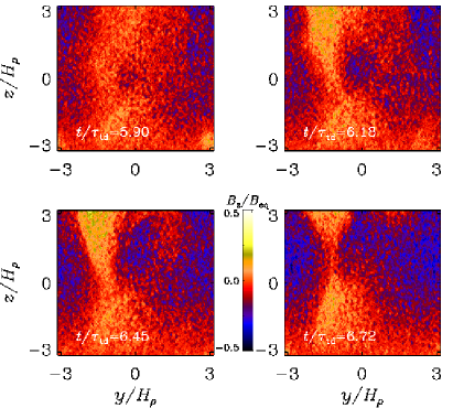
Figure 7: DNS for $\mbox{\rm Re}_{M}=260$ (Run R3): time evolution of $B_{z}/B_{\rm eq}$ in the $yz$ plane through $x/H_{\rho}=\pi$ for the fully helical run.

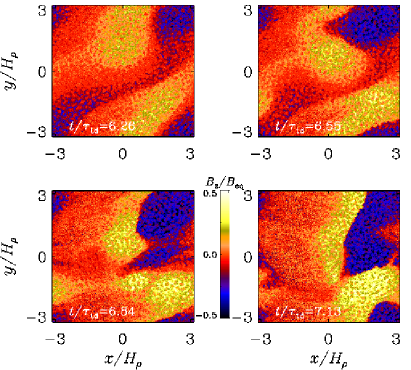
Figure 8: DNS for $\mbox{\rm Re}_{M}=260$ (Run R3): time evolution of $B_{z}/B_{\rm eq}$ in the $xy$ plane at the top surface for the fully helical run.

3.1.4 Higher Reynolds numbers and smaller scale separation

At larger values of $\mbox{\rm Re}_{M}$, the surface appearance of the field becomes more fragmented. This might be interesting in view of sunspot formation, since active regions appear to be more isolated than what one expects from a diffusive large-scale magnetic field.

Here we study the effects of varying the magnetic Reynolds number on the formation of structures in the one-layer model. In Figs. 7 and 8, we present the results for $\mbox{\rm Re}_{M}=260$. We recall that $\mbox{\rm Pr}_{M}$ was kept constant ($\mbox{\rm Pr}_{M}=0.5$), which implies that Re varies from 100 to up to 500 in these simulations. One can see from Fig. 4 that increasing the value of $\mbox{\rm Re}_{M}$ leads to a decrease in the amplitude of the nonlinear oscillations.

Next, we study the formation of sharp structures as seen in Fig. 3. For this purpose, we use $x$-averaged data because the resulting structure is independent of $x$ at the time the structure has developed. This does not apply to the run with the highest $\mbox{\rm Re}_{M}$ (Run R3) where the structure does depend on $x$; see Fig. 8.

To confirm that in our one-layer model the formation of the bipolar magnetic structures is independent of the value of the scale separation ratio, we now consider the case with $k_{\rm f}/k_{1}=5$ (Run R4). The main difference relative to our reference model is that the structures move faster and are more irregular. They also form at later times relative to the reference run with larger scale separation.

3.1.5 Effect of rotation

In this section we consider DNS of helically forced rotating turbulence. We see from Table LABEL:Tab1 that an increase in the rotation rate leads to a decrease in the growth rate of the dynamo when Co is of the order of unity (cf. Runs R5 and R6). However, even for $\mbox{\rm Co}=1.4$ (Run R7), sharp structures can still form, as was already emphasized in earlier work (Jabbari et al., 2016),

Owing to the presence of stratification, rotation leads to the additional production of kinetic helicity. Once rotation is fast enough, the resulting helicity will lead to an $\alpha$ effect that can be supercritical for dynamo action. We return to this at the end of the paper.

3.1.6 Energy spectra

Similar to earlier findings in strongly stratified layers (Brandenburg et al., 2014), there is a dramatic build-up of power at the largest scales of the domain. This was tentatively associated with inverse cascade-like behavior that could be related with the production of cross helicity, $\langle\mbox{\boldmath$u$}{}\cdot\bm{B}\rangle$, due to the presence of a mean magnetic field parallel or antiparallel to gravity. Indeed, strong cross helicity is also present in our current model, but its sign changes across the surface, because the mean vertical field changes; see Fig. 9.

The dramatic build-up of power at the largest scales is best demonstrated by plotting horizontal power spectra of $B_{z}(x,y)$ taken at the top of the domain during the formation of the structures; see Fig. 10. These spectra denote the energy in wavenumber shells of radius $k_{\perp}=(k_{x}^{2}+k_{y}^{2})^{1/2}$, and are normalized such that $\int E_{\rm M}^{z}(k_{\perp})\,{\rm d}{}k_{\perp}=\langle B_{z}^{2}\rangle/2$. Note that the ratio between the energy injection wavenumber and the wavenumber of the peak of the spectrum is equal to the scale separation ratio, $k_{\rm f}/k_{1}=30$.

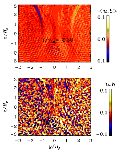
Figure 9: DNS for $\mbox{\rm Re}_{M}=50$ (Run R1): cross helicity density (upper panel) averaged along the $x$ direction. The lower panel shows the cross helicity at $x/H_{\rho}=0.5$.

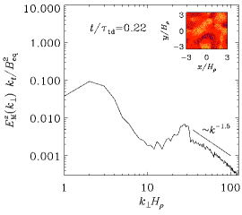
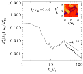
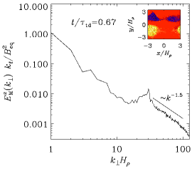
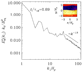
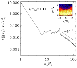
Figure 10: DNS for $\mbox{\rm Re}_{M}=50$ (Run R3): time evolution of $E_{\rm M}^{z}(k_{\perp})$ normalized by $B_{\rm eq}^{2}/k_{\rm f}$. The insets show the vertical field at the surface.

3.2 The dynamo in MFS

To understand the origin and nonlinear dynamics of the sharp structures found in the present DNS in the one-layer model and in the two-layer models of Mitra et al. (2014) and Jabbari et al. (2016), we start with a simple two-dimensional mean-field one-layer model with an algebraically quenched $\alpha$ effect and feedback from the self-generated large-scale magnetic field. In Sect. 3.4, we also consider a three-dimensional mean-field one-layer model. For simplicity, we have ignored here the dynamical nonlinearity caused by the evolution of the magnetic helicity. Furthermore, we have ignored algebraic quenching of the turbulent diffusivity. Since the dynamo growth is very rapid in DNS, we begin by neglecting in our mean-field model the effects of NEMPI, i.e., the effects of turbulence on the mean effective magnetic pressure. We do, however, include NEMPI in some of the 3D MFS; see Sect. 3.5.

3.2.1 Magnetic field evolution in MFS

Mean-field dynamo action begins when $C_{\alpha}>C_{\alpha}^{\rm crit}$, i.e., when $C_{\alpha}$ exceeds a critical value. Using 2D MFS we find that the dynamo threshold $C_{\alpha}^{\rm crit}\approx 2.55$; which agrees with the analytic value of $2.550650$ (Brandenburg, 2017). The cycles appear particularly pronounced in the rms velocity of the mean flow $\overline{\mbox{\boldmath$U$}}{}$, which excludes the small-scale flow that is implicitly present in the MFS in that it provides the turbulent diffusion. If this component is included, then the resulting total rms velocities show much less variation with the cycle. The cycle frequency for the marginally exited state is $\omega_{\rm cyc}=2\pi/P_{\rm cyc}\approx 1.43\tau_{\rm td}^{-1}$, where $P_{\rm cyc}\approx 4.4\tau_{\rm td}$ is the cycle period. Again, this is in good agreement with the analytic value of $1.429692$ (Brandenburg, 2017).

In the following, we fix $\mbox{\rm Pr}_{M}^{\rm turb}=1$ and $\mbox{\rm Fr}=0.05$. These values agree with those adopted in the DNS of Mitra et al. (2014) and Jabbari et al. (2016). The values of $C_{\alpha}$ and $C_{u}$ are harder to estimate from the DNS. We consider several cases that are listed in Table LABEL:TSum. The time evolutions of $\overline{U}_{\rm rms}/u_{\rm rms}$ and $\overline{B}_{\rm rms}/B_{\rm eq0}$ are shown in Fig. 11. In all cases, there are long-term oscillations with a period of approximately the turbulent-diffusive time. The cycle frequencies are listed in Table LABEL:TSum and compared with the marginally excited (linear) case, whose cycle frequency is less than those in all the nonlinear cases. As usual, the cycle frequency is determined from any of the nonvanishing components of $\overline{\mbox{\boldmath$B$}}{}$ and thus not from $\overline{B}_{\rm rms}$. The normalized frequencies increase slightly with increasing value of $C_{u}$; cf. Runs III-V in Table LABEL:TSum. The nonlinear oscillations are particularly pronounced in the mean flow. When the mean flow reaches a maximum, the mean magnetic field strength decreases slightly. It is seen in Fig. 11 that the minima of the rms value of the mean velocity during the cycle are much deeper than those of the mean magnetic field.

Table 2: Summary of MFS; ‘marg’ refers to the marginally excited case, which is independent of the values of $C_{u}$ and $Q_{\alpha}$.

Case $C_{\alpha}$ $C_{u}$ $Q_{\alpha}$ $\omega_{\rm cyc}\,\tau_{\rm td}$ $\overline{B}_{\rm rms}/B_{\rm eq0}$ I 20 40 1 3.08 0.32 I3D 20 40 1 6.23 0.33 II 10 40 1 2.38 0.20 II’ 10 40 0.3 2.68 0.37 II3D 10 40 1 4.5 0.20 II3D-rot 10 40 1 1.9 0.21 III 10 80 1 3.11 0.19 IV 10 160 1 3.62 0.19 V 10 320 1 4.04 0.19 VI3D 5 40 1 1.8 0.11 VI3D-NEMPI 5 40 1 1.53 0.11 marg 2.55 — — 1.43 —

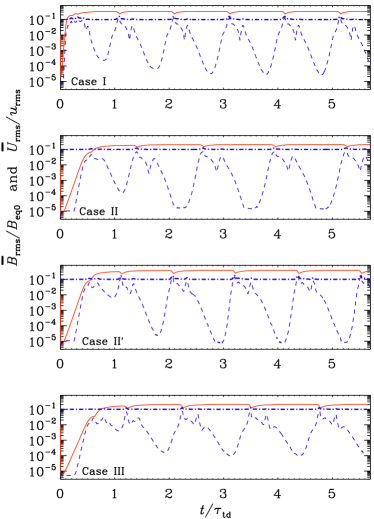
Figure 11: 2D MFS: $\overline{B}_{\rm rms}/B_{\rm eq0}$ (solid red) and $\overline{U}_{\rm rms}/u_{\rm rms}$ (dashed blue) vs. time. The fat dash-dotted line gives the total rms velocity, which includes the contribution from $u_{\rm rms}$.

In Fig. 12 we show four snapshots of $\overline{B}_{z}$ together with vectors of $\overline{\mbox{\boldmath$U$}}{}$ in the $xz$ plane during the time when the mean flow reaches its maximum. The maxima in $\overline{U}_{\rm rms}$ correspond to times when a strong downflow develops. As is evident from Fig. 12, these flows push fields of opposite sign together and form a current sheet in the uppermost layer, which then leads to a downflow. This destroys most of the field through turbulent diffusion (or turbulent reconnection), but it is soon being replenished by dynamo action from the deeper layers.

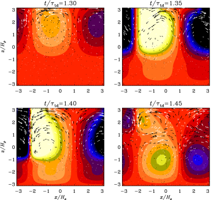
Figure 12: 2D MFS: snapshots of $\overline{B}_{z}$ (color-coded) together with vectors of $\overline{\mbox{\boldmath$U$}}{}$ in the $xz$ plane for case II during the time when the mean flow reaches its maximum. Note the sharp structure at $t/\tau_{\rm td}=1.40$.

In our model, the $\alpha$ quenching with $Q_{\alpha}=1$ limits the field strength to values just below the local equipartition value. This is clear from Fig. 13, where we show $\overline{B}_{z}^{2}/B_{\rm eq}^{2}$ versus $x/H_{\rho}$ for $z/H_{\rho}=3$, $2$, and $1$. The plasma-$\beta$ of the vertical field defined as $\mu_{0}\overline{\rho}c_{\rm s}^{2}/\overline{B}_{z}^{2}$, reaches minimum values of around 10. However, in the modified model (case II’) with $Q_{\alpha}=0.3$, the minimum plasma-$\beta$ reaches values of about 2; see Fig. 14. In fact, even smaller values of $Q_{\alpha}$ down to 0.11 have been found in rotating convection using the test-field method; see Karak et al. (2014).

Figure 13: 2D MFS: $\overline{\mbox{\boldmath$B$}}{}^{2}/B_{\rm eq}^{2}$ (left axis) and plasma-$\beta$ (right axis) as a function of $x/H_{\rho}$ for $t/\tau_{\rm td}=1.40$ through $z/H_{\rho}=3$ (solid line), $2$ (dashed line), and $1$ (dotted line) for case II. The $x$ axis has been extended periodically to smaller values.

Figure 14: 2D MFS: similar to Fig. 13, but for case II’.

Figure 15: DNS for $\mbox{\rm Re}_{M}=50$ (Run R1): $\overline{\mbox{\boldmath$B$}}{}^{2}/B_{\rm eq}^{2}$ as a function of $y/H_{\rho}$ for $t/\tau_{\rm td}=2.50$ through $z/H_{\rho}=3$ (solid line), $2$ (dashed line), and $1$ (dotted line).

3.2.2 Height dependence of sharp structures

The sharp structures are particularly pronounced in the upper, low density regions. We have seen this already in Figs. 13 and 14, where we show $\overline{B}_{z}^{2}/B_{\rm eq}^{2}$ for three values of $z/H_{\rho}$ as a function of $y$. The same behavior is also seen in the DNS in Fig. 15, where we plot the same quantity, which is now shown as an $x$-averaged quantity at the time $t/\tau_{\rm td}=2.50$, when the magnetic structures are sharpest. Comparing with Figs. 13 and 14, we also see that the larger values of $\overline{B}_{z}^{2}/B_{\rm eq}^{2}$ in the DNS are best matched for a smaller value of $Q_{\alpha}$.

To demonstrate that the sharp structures are caused by the Lorentz force, particularly the mean magnetic pressure gradient, we compare in Fig. 16 the surface profiles (at $z/H_{\rho}=\pi$) of mean gas pressure $\overline{p}_{\rm gas}=\overline{\rho}c_{\rm s}^{2}$, mean magnetic pressure $\overline{p}_{\rm mag}=\overline{\mbox{\boldmath$B$}}{}^{2}/2$ (shifted upward by a constant, which is here the horizontally averaged mean gas pressure at the surface, $\langle\overline{p}_{\rm gas}\rangle$), and mean total pressure, $\overline{p}_{\rm gas}+\overline{p}_{\rm mag}$. The gas pressure gradient is always directed away from the sharp structure and opposes its formation. The mean magnetic pressure gradient is directed toward the sharp structure and overcomes the mean gas pressure gradient at the time when the structure forms.

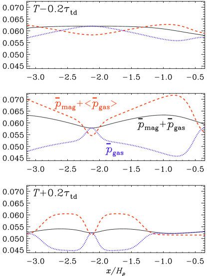
Figure 16: 2D MFS for case II’ showing the mean pressure balance at the surface at three times: $t=T-0.2\tau_{\rm td}$ (upper panel), $t=T$ (middle panel), and $t=T+0.2\tau_{\rm td}$ (lower panel), around the moment when the mean magnetic pressure gradient is largest (at $t\equiv T$).

3.3 Similarity between DNS and MFS

The sharp structures appear superficially similar to those found by Mitra et al. (2014) and Jabbari et al. (2016). In the present case, a sharp structure is seen to appear at $t/\tau_{\rm td}=1.35$ and it disappears already at $t/\tau_{\rm td}=1.45$. However, in units of $\tau_{\rm td}^{\prime}$, which are the units used by Mitra et al. (2014) and Jabbari et al. (2016), the corresponding time interval is of the order of unity and thus compatible with Mitra et al. (2014) and Jabbari et al. (2016), where the sharp structures persist and appear to “stick” together for the duration of $\tau_{\rm td}^{\prime}$.

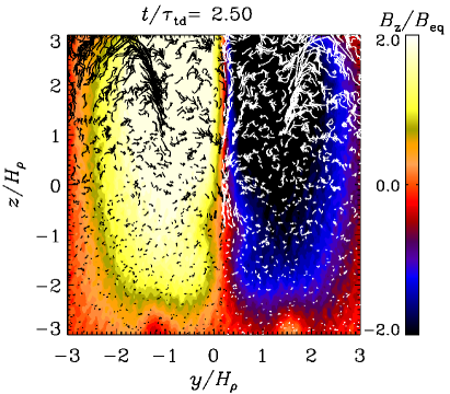
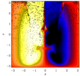
Figure 17: $\overline{B}_{z}/B_{\rm eq}$, together with $\overline{u}_{y}/B_{\rm eq}$ and $\overline{u}_{z}/B_{\rm eq}$ vectors for the fully helical run to compare DNS for $\mbox{\rm Re}_{M}=50$ (upper panel, Run R1) with MFS (lower panel, Run II).

We recall that we have assumed $\alpha_{0}={\rm const}{}$, i.e., the $\alpha$ effect is independent of $z$. This is appropriate for simulating a one-layer system, in particular Run RM1zs of Jabbari et al. (2016). The value of $C_{\alpha}$ is therefore essentially determined by the scale separation ratio, $k_{\rm f}/k_{1}$; see Jabbari et al. (2014). Furthermore, the value of $C_{u}$ can be estimated by using the mean-field expression $\eta_{\rm T}\approx u_{\rm rms}/3k_{\rm f}$, which yields $C_{u}=3k_{\rm f}/\tilde{k}_{1}$. Mitra et al. (2014) and Jabbari et al. (2016) used $k_{\rm f}/k_{1}=30$ and since $\tilde{k}_{1}=k_{1}/4$, their value is $C_{u}=360$, which is larger than those considered here.

Fig. 17 shows a comparison of the magnetic structure together with velocity vectors in DNS (upper panel) with MFS (lower panel). One can see that the location of converging flow structures and downdrafts is similar in both DNS and MFS.

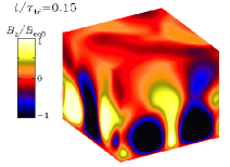
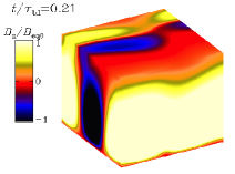
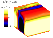
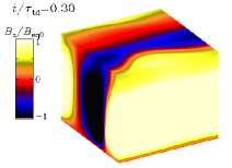
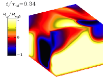
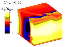
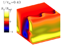
Figure 18: Visualization of $\overline{B}_{z}/B_{\rm eq0}$ on the periphery of the computational domain for Run I3D (3D MFS).

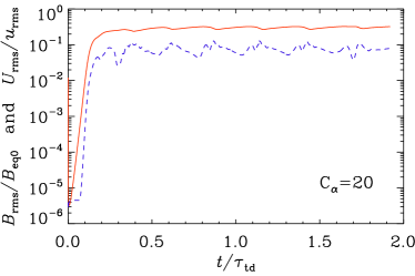
Figure 19: $\overline{B}_{\rm rms}/B_{\rm eq0}$ (solid red) and $\overline{U}_{\rm rms}/u_{\rm rms}$ (dashed blue) vs. time for Run I3D (3D MFS).

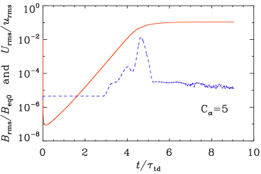
Figure 20: $\overline{B}_{\rm rms}/B_{\rm eq0}$ (solid red) and $\overline{U}_{\rm rms}/u_{\rm rms}$ (dashed blue) vs. time for Run VI3D (3D MFS with weak dynamo).

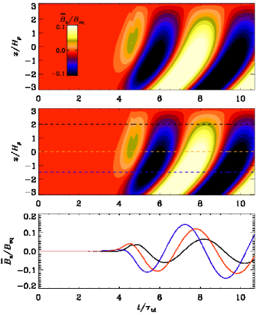
Figure 21: MFS weak dynamo: butterfly diagrams $\overline{B}(x_{c},y_{c},z,t)/B_{\rm eq}(z)$ for Run VI3D through cross-sections $x_{c}/H_{\rho}=\pi$, and either $y_{c}/H_{\rho}=0.$ (top panel) or $1.8$ (middle panel), as well as $\overline{B}_{x}(x_{c},y_{c},z_{c},t)/B_{\rm eq}$ through $x_{c}/H_{\rho}=\pi$ and $y_{c}/H_{\rho}=1.8$ for $z_{c}/H_{\rho}=2$ (black line), $z_{c}/H_{\rho}=-1.5$ (blue line), and $z_{c}/H_{\rho}=0.$ (red line) versus time (lower panel). In the second panel the dashed black, red, and blue horizontal lines show the locations where $\overline{B}_{x}(x_{c},y_{c},z_{c},t)/B_{\rm eq}$ is plotted vs. $t$.

3.4 Three-dimensional MFS

As seen in the DNS, the magnetic structures are not two-dimensional at all times. It is therefore important to perform mean-fields calculations also in three dimensions. The result is shown in Fig. 18, where we plot the $z$ component of the magnetic field on the periphery of the domain. Looking at an animation, one can see that magnetic structures rotate in the counterclockwise direction. This direction would be the other way around in a model with negative $\alpha$ effect. We also see (e.g., at $t/\tau_{\rm td}=0.43$) that the reconnection layers tend to develop Kelvin-Helmholtz instabilities corresponding to shear flows that have the same sense as in the two-dimensional simulations.

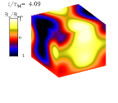
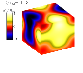
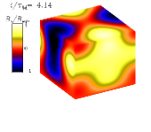
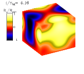
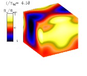
Figure 22: Visualization of $\overline{B}_{z}/B_{\rm eq0}$ on the periphery of the computational domain for Run VI3D (3D MFS with weak dynamo).

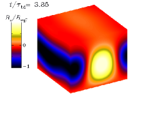
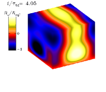
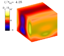
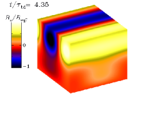
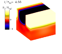
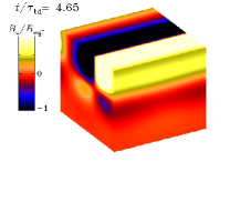
Figure 23: Time evolution of $\overline{B}_{z}/B_{\rm eq}$ in the box for $C_{\alpha}=5$ with NEMPI parameterization for Run VI3D-NEMPI (3D MFS).

Compared with the two-dimensional MFS, the period of oscillations is now almost three times shorter than in the two-dimensional calculations; see Fig. 19. This is surprising and suggests that the nonlinearity from the feedback via the mean-field momentum equation is rather important. Compared with the DNS, the period is larger still. This nonlinearity might therefore be even more important in the DNS and that in the MFS the nonlinearity from algebraic $\alpha$ quenching may be overestimated, i.e., the parameter $Q_{\alpha}$ was chosen too large. Compared with Fig. 11, the minima are now much shallower.

In case VI3D with the lower dynamo number ($C_{\alpha}=5$, “weak dynamo”), the values of $\overline{B}_{\rm rms}$ and $\overline{U}_{\rm rms}$ become approximately constant, with $\overline{U}_{\rm rms}/u_{\rm rms}$ being much smaller than before; see Fig. 20. Nevertheless, the dynamo-generated magnetic field remains oscillatory, as can be seen from the butterfly diagram in Fig. 21. This is consistent with earlier results of Brandenburg et al. (2009). Another interesting result of employing a lower value of $C_{\alpha}$ is presented in Fig. 22, where we show $\overline{B}_{z}/B_{\rm eq0}$ on the periphery of the domain for Run VI3D. One can see the clear formation of an X-point during the reconnection of magnetic field lines at the surface of the box (see the third panel).

Next, we perform a 3D MFS study with rotation by including the Coriolis force in the mean momentum equation (Run II3D-rot in Table LABEL:TSum). Similarly to the DNS, magnetic structures are formed in the presence of rotation. As one can see from Table LABEL:TSum, the cycle frequency in this case is two times smaller in comparison with the non-rotating run with similar parameters. On the other hand, the cycle frequency observed in the 3D rotating MFS is nearly the same as in the 2D MFS with similar parameters.

3.5 3D MFS with NEMPI

To compare with the 3D MFS described in Sect. 3.4, we now include the parameterization of NEMPI by the following replacement of the mean Lorentz force in Eq. (8).

$$\overline{\mbox{\boldmath$J$}}{}\times\overline{\mbox{\boldmath$B$}}{}\to\overline{\mbox{\boldmath$J$}}{}\times\overline{\mbox{\boldmath$B$}}{}+\mbox{\boldmath$\nabla$}{}\left({\textstyle{1\over 2}}q_{\rm p}\overline{\mbox{\boldmath$B$}}{}^{2}\right),$$ (19)

where $q_{\rm p}$ determines the turbulence contribution to the large-scale Lorentz force. Here, $q_{\rm p}$ depends on the local field strength and is approximated by (Kemel et al., 2012)

$$q_{\rm p}(\beta)={q_{\rm p0}\over 1+\beta^{2}/\beta_{\rm p}^{2}},$$ (20)

where $q_{\rm p0}$ and $\beta_{\rm p}$ are constants, and $\beta=|\overline{\mbox{\boldmath$B$}}{}|/B_{\rm eq}$ is the normalized mean magnetic field. For $\mbox{\rm Re}_{M}\mathrel{\mathchoice{\vbox{\offinterlineskip\halign{\hfil$\displaystyle#$\hfil\cr<\cr\sim\cr}}}{\vbox{\offinterlineskip\halign{\hfil$\textstyle#$\hfil\cr<\cr\sim\cr}}}{\vbox{\offinterlineskip\halign{\hfil$\scriptstyle#$\hfil\cr<\cr\sim\cr}}}{\vbox{\offinterlineskip\halign{\hfil$\scriptscriptstyle#$\hfil\cr<\cr\sim\cr}}}}60$, Brandenburg et al. (2012) found $q_{\rm p0}\approx 32$ and $\beta_{\rm p}\approx 0.058$.

NEMPI describes the formation of magnetic structures through a strong reduction of turbulent pressure by the large-scale magnetic field. For large magnetic Reynolds numbers, this suppression of the turbulent pressure can be strong enough so that the effective large-scale magnetic pressure (the sum of non-turbulent and turbulent contributions to the large-scale magnetic pressure) can become negative. This results in the excitation of a large-scale hydromagnetic instability, namely NEMPI. In Fig. 23 we show the time evolution of $\overline{B}_{z}/B_{\rm eq}$ on the periphery of the computational domain for $C_{\alpha}=5$ with the NEMPI parameterization included (Run VI3D-NEMPI). In this case we also observe the formation of bipolar magnetic structures, but now mainly in the upper parts of the computational domain.

3.6 Combined effect of rotation and stratification in DNS

We now investigate a system of stratified, non-helically forced turbulence in the presence of rotation. We study the generation of a large-scale magnetic field driven by the $\alpha$ effect as a result of the combined effects of rotation and stratification. Jabbari et al. (2014) have studied a similar system, but in their case there was also a weak imposed horizontal magnetic field. Table LABEL:Tab3 shows all non-helical DNS runs with their parameters.

Table 3: Summary of the DNS with rotation and non-helical forcing. The reference run is shown in bold.

Run $\Omega$ Co $\theta$ $\mbox{\rm Re}_{M}$ $\tilde{\lambda}$ Rn1 2 1.4 0 58 0.097 Rn2 2 1.4 180 56 0.098 Rn3 2 1.4 45 61 0.087 Rn4 2 1.4 90 65 0.086 Rn5 4 2.8 0 68 0.113 Rn6 8 5.6 0 81 0.107 Rn7 10 6.7 0 99 0.098

Figure 24: $\langle\mbox{\boldmath$\omega$}{}\cdot\mbox{\boldmath$u$}{}\rangle/k_{\rm f}u_{\rm rms}^{2}$, $\mu_{0}\langle\mbox{\boldmath$J$}{}\cdot\bm{B}\rangle/k_{\rm f}u_{\rm rms}^{2}$, $\langle B_{x}\rangle/B_{\rm eq}(z)$, and $\langle B_{y}\rangle/B_{\rm eq}(z)$ as a function of $z/H_{\rho}$ and $t/\tau_{\rm td}$ for Run Rn6 (DNS of non-helically forced rotating turbulence).

We have performed a number of runs with varying Coriolis number, Co. We also vary colatitude $\theta$ (Runs Rn2–4). Our simulations show that for fast rotation ($\mbox{\rm Co}>5.6$) and for $\theta=0$ (Runs Rn6 and Rn7), the self-generated kinetic helicity leads to an $\alpha^{2}$ dynamo. At a later stage, bipolar magnetic structures form. Fig. 24 presents the time evolution of kinetic and magnetic helicities together with the horizontal components of the magnetic field. One can see the production of negative kinetic helicity in almost all of the entire domain (see the upper left panel of Fig. 24). Magnetic helicity, however, has both negative and positive signs and has a non-zero value in the lower part of the domain (see the upper right panel of Fig. 24). In the lower row of Fig. 24, we present the butterfly diagram of $B_{x}/B_{\rm eq}(z)$ (left), and $B_{y}/B_{\rm eq}(z)$ (right). There is a clear phase shift between these two field components, similar to what one expects from a Beltrami-type magnetic field driven by $\alpha^{2}$ dynamo. This large-scale magnetic field reaches the surface and bipolar magnetic spots are formed; see Fig. 25.

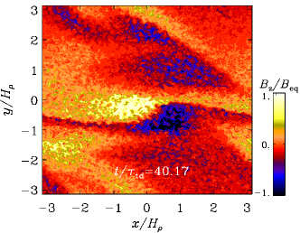
Figure 25: $B_{z}/B_{\rm eq}$ in the $xy$ plane through $z/H_{\rho}=\pi$ for DNS Run Rn6 with non-helically forced rotating turbulence.

4 Conclusions

In this work we have compared DNS of helically forced turbulence in a strongly stratified layer with corresponding MFS. Compared with earlier DNS (Mitra et al., 2014; Jabbari et al., 2016), we have considered here a one-layer model and have shown that this simpler case also leads to the formation of sharp bipolar structures at the surface. Larger values of $\mbox{\rm Re}_{M}$ result in more complex spatio-temporal behavior, while rotation (with $\mbox{\rm Co}\mathrel{\mathchoice{\vbox{\offinterlineskip\halign{\hfil$\displaystyle#$\hfil\cr<\cr\sim\cr}}}{\vbox{\offinterlineskip\halign{\hfil$\textstyle#$\hfil\cr<\cr\sim\cr}}}{\vbox{\offinterlineskip\halign{\hfil$\scriptstyle#$\hfil\cr<\cr\sim\cr}}}{\vbox{\offinterlineskip\halign{\hfil$\scriptscriptstyle#$\hfil\cr<\cr\sim\cr}}}}1$) and the scale separation ratio have only minor effects. Both aspects confirm similar findings for our earlier two-layer model.

The results of our MFS are generally in good qualitative agreement with the DNS. The MFS without parameterized NEMPI (i.e., neglecting the turbulence effects on the Lorentz force) demonstrate that the formation of sharp structures at the surface occurs predominantly due to the nonlinear effects associated with the mean Lorentz force of the dynamo-generated magnetic field, provided the dynamo number is at least 2.5 times supercritical. This results in converging flow structures and downdrafts in equivalent locations both in DNS and MFS. For smaller dynamo numbers, when the field strength is below equipartition, NEMPI can operate and form bipolar regions, as was shown in earlier DNS (Warnecke et al., 2013, 2016). Comparing MFS without and with inclusion of the parameterization of NEMPI by replacing the mean Lorentz force with the effective Lorentz force in the Navier-Stokes equation, we found that the formation of bipolar magnetic structures in the case of NEMPI is also accompanied by downdrafts, especially in the upper parts of the computational domain.

In this connection, we recall that our system lacks the effects of thermal buoyancy, so our downdrafts are distinct from those in convection. In the Sun, both effects may contribute to driving convection, especially on the scale of supergranulation. However, from convection simulations with and without magnetic fields, no special features of magnetically driven downflows have been seen (Käpylä et al., 2016).

Finally, we have considered nonhelically forced turbulence, but now with sufficiently rapid rotation which, together with density stratification, leads to an $\alpha$ effect that is supercritical for the onset of dynamo action. Even in that case we find the formation of sharp bipolar structures. They begin to resemble the structures of bipolar regions in the Sun. Thus, we may conclude that the appearance of bipolar structures at the solar surface may well be a generic feature of a large scale dynamo some distance beneath the surface of a strongly stratified domain.

As a next step, it will be important to consider more realistic modeling of the large-scale dynamo. This can be done in global spherical domains with differential rotation, which should lead to preferential east-west alignment of the bipolar structures. In addition, the effects of convectively-driven turbulence would be important to include. This would automatically account for the possibility of thermally driven downflows, in addition to just magnetically driven flows. In principle, this has already been done in the many global dynamo simulations performed in recent years (Brown et al., 2011; Käpylä et al., 2012; Fan & Fang, 2014; Hotta et al., 2016), but in most of them the stratification was not yet strong enough and the resolution insufficient to resolve small enough magnetic structures at the surface.

The spontaneous formation of magnetic surface structures from a large-scale $\alpha^{2}$ dynamo by strongly stratified thermal convection in Cartesian geometry has recently also been studied by Masada & Sano (2016). They found that large-scale magnetic structures are formed at the surface only in cases with strong stratification. However, in many other convection simulations, the scale separation between the integral scale of the turbulence and the size of the domain is not large enough for the formation of sharp magnetic structures. One may therefore hope that future simulations will not only be more realistic, but will also display surface phenomena that are closer to those observed in the Sun.

References

- Birch et al. (2016) Birch, A. C., Schunker, H., Braun, D. C., Cameron, R., Gizon, L. Löptien, B., & Rempel, M. 2016, Sci. Adv. 2, e1600557
- Brandenburg (2001) Brandenburg, A. 2001, ApJ, 550, 824
- Brandenburg (2017) Brandenburg, A. 2017, A&A, 598, A117
- Brandenburg et al. (2009) Brandenburg, A., Candelaresi, S., & Chatterjee, P. 2009, MNRAS, 398, 1414
- Brandenburg et al. (2014) Brandenburg, A., Gressel, O., Jabbari, S., Kleeorin, N., & Rogachevskii, I. 2014, A&A, 562, A53
- Brandenburg et al. (2011) Brandenburg, A., Kemel, K., Kleeorin, N., Mitra, D., Rogachevskii, I. 2011, ApJ, 740, L50
- Brandenburg et al. (2012) Brandenburg, A., Kemel, K., Kleeorin, N., Rogachevskii, I. 2012, ApJ, 749, 179
- Brandenburg et al. (2010) Brandenburg, A., Kleeorin, N., & Rogachevskii, I. 2010, Astron. Nachr., 331, 5
- Brandenburg et al. (2013) Brandenburg, A., Kleeorin, N., & Rogachevskii, I. 2013, ApJ, 776, L23
- Brandenburg et al. (2016) Brandenburg, A., Rogachevskii, I., & Kleeorin, N. 2016, NJP, 18, 125011
- Brown et al. (2011) Brown, B. P., Miesch, M. S., Browning, M. K., Brun, A. S., Toomre, J. 2011, ApJ, 731, 69
- Caligari et al. (1995) Caligari, P., Moreno-Insertis, F., & Schüssler, M. 1995, ApJ, 441, 886
- Fan (2001) Fan, Y. 2001, ApJ, 554, L111
- Fan (2008) Fan, Y. 2008, ApJ, 676, 680
- Fan & Fang (2014) Fan, Y., & Fang, F. 2014, ApJ, 789, 35
- Higham (2001) Higham D., 2001, SIAM Review, 43, 525
- Hotta et al. (2016) Hotta, H., Rempel, M., & Yokoyama, T. 2016, Science, 351, 1427
- Iroshnikov (1971) Iroshnikov, R. S. 1971, Sov. Astron., 14, 1001
- Jabbari et al. (2013) Jabbari, S., Brandenburg, A., Kleeorin, N., Mitra, D., & Rogachevskii, I. 2013, A&A, 556, A106
- Jabbari et al. (2014) Jabbari, S., Brandenburg, A., Losada, I. R., Kleeorin, N., & Rogachevskii, I. 2014, A&A, 568, A112
- Jabbari et al. (2015) Jabbari, S., Brandenburg, A., Kleeorin, N., Mitra, D.,& Rogachevskii, I. 2015, ApJ, 805, 166
- Jabbari et al. (2016) Jabbari, S., Brandenburg, A., Mitra, D., Kleeorin, N., & Rogachevskii, I. 2016, MNRAS, 459, 4046
- Jouve & Brun (2009) Jouve, L., Brun, A. S. 2009, ApJ, 701, 1300
- Käpylä et al. (2012) Käpylä, P. J., Mantere, M. J., & Brandenburg, A. 2012, ApJ, 755, L22
- Käpylä et al. (2012) Käpylä, P. J., Brandenburg, A., Kleeorin, N., Mantere, M. J., & Rogachevskii, I. 2012, MNRAS, 422, 2465
- Käpylä et al. (2016) Käpylä, P. J., Brandenburg, A., Kleeorin, N., Käpylä, M. J., & Rogachevskii, I. 2016, A&A, 588, A150
- Karak et al. (2014) Karak, B. B., Rheinhardt, M., Brandenburg, A., Käpylä, P. J., & Käpylä, M. J. 2014, ApJ, 795, 16
- Kemel et al. (2012) Kemel, K., Brandenburg, A., Kleeorin, N., & Rogachevskii, I. 2012, Astron. Nachr., 333, 95
- Kleeorin et al. (1993) Kleeorin, N., Mond, M., & Rogachevskii, I. 1993, Phys. Fluids B, 5, 4128
- Kleeorin et al. (1996) Kleeorin, N., Mond, M., & Rogachevskii, I. 1996, A&A, 307, 293
- Kleeorin & Rogachevskii (1994) Kleeorin, N., & Rogachevskii, I. 1994, Phys. Rev. E, 50, 2716
- Kleeorin et al. (1989) Kleeorin, N.I., Rogachevskii, I.V., & Ruzmaikin, A.A. 1989, Sov. Astron. Lett., 15, 274
- Kleeorin et al. (1990) Kleeorin, N. I., Rogachevskii, I. V., Ruzmaikin, A. A. 1990, Sov. Phys. JETP, 70, 878
- Masada & Sano (2016) Masada, Y., & Sano, T. 2016, ApJ, 822, L22
- Mitra et al. (2010) Mitra, D., Tavakol, R., Käpylä, P. J., & Brandenburg, A. 2010, ApJ, 719, L1
- Mitra et al. (2014) Mitra, D., Brandenburg, A., Kleeorin, N., Rogachevskii, I. 2014, MNRAS, 445, 761
- Parker (1955) Parker, E. N. 1955, ApJ, 121, 491
- Parker (1975) Parker, E. N. 1975, ApJ, 198, 205
- Rogachevskii & Kleeorin (2007) Rogachevskii, I., & Kleeorin, N. 2007, Phys. Rev. E, 76, 056307
- Warnecke et al. (2011) Warnecke, J., Brandenburg, A., & Mitra, D. 2011, A&A, 534, A11
- Warnecke et al. (2013) Warnecke, J., Losada, I. R., Brandenburg, A., Kleeorin, N., & Rogachevskii, I. 2013, ApJ, 777, L37
- Warnecke et al. (2016) Warnecke, J., Losada, I. R., Brandenburg, A., Kleeorin, N., & Rogachevskii, I. 2016, A&A, 589, A125