Convergence and Cycling in Walker-type Saddle Search Algorithms

Abstract

Algorithms for computing local minima of smooth objective functions enjoy a mature theory as well as robust and efficient implementations. By comparison, the theory and practice of saddle search is destitute. In this paper we present results for idealized versions of the dimer and gentlest ascent (GAD) saddle search algorithms that show-case the limitations of what is theoretically achievable within the current class of saddle search algorithms: (1) we present an improved estimate on the region of attraction of saddles; and (2) we construct quasi-periodic solutions which indicate that it is impossible to obtain globally convergent variants of dimer and GAD type algorithms.

1 Introduction

The first step in the exploration of a molecular energy landscape is usually the determination of energy minima, using an optimization algorithm. There exists a large number of such algorithms, backed by a rich and mature theory [9, 2]. Virtually all optimization algorithms in practical use today feature a variety of rigorous global and local convergence guarantees, and well-understood asymptotic rates.

As a second step, one typically determines the saddles between minima. They represent a crude description of the transitions between minima (reactions) and can be thought of as the edges in the graph between stable states of a molecule or material system. If neighboring minima are known, then methods of NEB or string type [8, 3] may be employed. On the other hand when only one minimum is known, then “walker methods” of the eigenvector-following methodology such as the dimer algorithm [7] are required. This second class of methods is the focus of the present work; for extensive reviews of the literature we refer to [10, 4, 1, 6].

Since saddles represent reactions, the determination of saddle points is of fundamental importance in determining dynamical properties of an energy landscape, yet the state of the art of algorithms is very different from that for optimization: more than 15 years after the introduction of the dimer method [7] (the most widely used walker-type saddle search scheme), finding saddle points remains an art rather than a science. A common practice is to detect non-convergence and restart the algorithm with a different starting point. A mathematically rigorous convergence theory has only recently begun to emerge; see [12, 6] and references therein. To the best of our knowledge all convergence results to date are local: convergence can only be guaranteed if an initial guess is sufficiently close to a (index-1) saddle. None of the existing saddle search algorithms come with the kind of global convergence guarantees that even the most basic optimization algorithms have.

The purpose of the present work is twofold: (1) We strengthen existing local convergence results for dimer/GAD type saddle search methods by developing an improved estimate on the region of attraction of index-1 saddle points that goes beyond the linearized regime. (2) We produce new examples demonstrating generic cycling in those schemes, and pathological behavior of idealized versions of these algorithms. These results illustrate how fundamentally different saddle search is from optimization. They suggest that a major new idea is required to obtain globally convergent walker-type saddle search methods, and support the idea of string-of-state methods being more robust.

1.1 Local and global convergence in optimization

We consider the steepest descent method as a prototype optimization algorithm. Given an energy landscape $E\in C^{2}(\mathbb{R}^{N})$, the gradient descent dynamics (or gradient flow) is

$$\dot{x}=-\nabla E(x).$$ (1)

This ODE enjoys the property that

$$\frac{\operatorname{d\!}}{\operatorname{d\!}t}E(x) =\left\langle\dot{x},\nabla E(x)\right\rangle=-\|\nabla E(x)\|^{2}.$$

If $E$ is bounded from below, it follows that $\nabla E(x)\to 0$ and, under mild conditions (for instance, $E$ coercive with non-degenerate critical points), $x$ converges to a critical point, that is generically a minimum.

This property can be transferred to the discrete iterates of the steepest descent method

$$x_{n+1}=x_{n}-\alpha_{n}\nabla E(x_{n}),$$ (2)

under conditions on the step length $\alpha_{n}$ (for instance the Armijo condition). In both cases, the crucial point for convergence is that $E(x(t))$ or $E(x_{n})$ is an objective function (also called merit or Lyapunov function) that decreases in time.

1.2 Eigenvector-following methods: the ISD and GAD

If $x_{*}$ is a non-degenerate index-1 saddle, then the symmetric Hessian matrix $H_{*}=\nabla^{2}E(x_{*})$ has one negative eigenvalue, while all other eigenvalues are positive. In this case, the steepest descent dynamics (1) is repelled away from $x_{*}$ along the mode corresponding to the negative eigenvalue.

To obtain a dynamical system for which $x_{*}$ is an attractive fixed point, we reverse the flow in the direction of the unstable mode. Let $v_{1}(x)$ be a normalized eigenvector corresponding to the smallest eigenvalue of $\nabla^{2}E(x)$, then for $\|x-x_{*}\|$ sufficiently small, the direction

$$-(I-2v_{1}(x)\otimes v_{1}(x))\nabla E(x)$$

points towards the saddle $x_{*}$. Note that this direction does not depend on the arbitrary sign of $v_{1}$, and therefore in the rest of the paper we will talk of “the lowest eigenvector $v_{1}(x)$” whenever the first eigenvalue of $\nabla^{2}E(x)$ is simple.

This is the essence of the eigenvector-following methodology, which has many avatars (such as the dimer method [7], the Gentlest Ascent Dynamics [4], and numerous variants). In our analysis we will consider the simplest such method, which we will call the Idealized Saddle Dynamics (ISD),

$$\dot{x}=-(I-2v_{1}(x)\otimes v_{1}(x))\nabla E(x).$$ (3)

Under this dynamics, a linear stability analysis shows that non-degenerate index-1 saddle points are attractive, while non-degenerate minima, maxima or saddle points of index greater than 1 are repulsive (see Lemma 1).

The ISD (3) is only well-defined when $v_{1}(x)$ is determined unambiguously, that is, when the first eigenvalue of $\nabla^{2}E(x)$ is simple. The singularities of this flow where $\nabla^{2}E(x)$ has repeated first eigenvalues will play an important role in this paper.

In practice, the orientation $v_{1}(x)$ has to be computed from $\nabla^{2}E(x)$. This makes the method unattractive for many applications in which the second derivative is not available or prohibitively expensive (for instance, ab initio potential surfaces, in which $E(x)$ and $\nabla E(x)$ are readily computed but $\nabla^{2}E(x)$ requires a costly perturbation analysis). Because of this, the orientation is often relaxed and computed in alternation with the translation (3). A mathematically simple flavor of this approach is the

Gentlest Ascent Dynamics (GAD): [4]

$$\begin{split}\dot{x}&=-(I-2v\otimes v)\nabla E(x),\\ \varepsilon^{2}\dot{v}&=-(I-v\otimes v)\nabla^{2}E(x)v.\end{split}$$ (4)

At a fixed $x$, the dynamics for $v$ is a gradient flow for the Rayleigh quotient $\left\langle v,\nabla^{2}E(x)v\right\rangle$ on the unit sphere $S_{1}$ in $\mathbb{R}^{N}$, which converges to the lowest eigenvector $v_{1}(x)$. The parameter $\varepsilon>0$ controls the speed of relaxation of $v$ towards $v_{1}(x)$ relative to that of $x$. The ISD is formally obtained in the limit $\varepsilon\to 0$.

The practical advantage of the GAD (4) over the ISD (3) is that, once discretized in time, it can be implemented using only the action of $\nabla^{2}E(x)$ on a vector, which can be computed efficiently via finite differences. This is the basis of the dimer algorithm [7]. The $\varepsilon$ scaling is analogous to common implementations of the dimer algorithm that adapt the number of rotations per step to ensure approximate equilibration of $v$.

Using linearized stability analysis one can prove local convergence of the ISD, GAD or dimer algorithms [12, 6]. However, due to the absence of a global merit function as in optimization, there is no natural Armijo-like condition to choose the stepsizes in a robust manner, or indeed to obtain global convergence guarantees (however, see [6, 5] for ideas on the construction of local merit functions).

In this paper, we only study the ISD and GAD dynamics: we expect that the behavior we find applies to practical variants under appropriate conditions on the parameters (for instance, the dimer algorithm with a sufficiently small finite difference step and a sufficiently high number of rotation steps per translation step).

1.3 Divergence of ISD-type methods

Even though dimer/GAD type methods converge locally under reasonable hypotheses, global convergence is out of reach. We briefly summarize two examples from [6, 4] to motivate our subsequent results.

One of the simplest examples is the 1D double-well [6]

$$E(x)=(1-x^{2})^{2}.$$ (5)

On this one-dimensional landscape, the ISD (3) is the gradient ascent dynamics. It converges to the saddle at $x=0$ if and only if started with $|x_{0}|<1$. If started from $|x_{0}|>1$, it will diverge to $\pm\infty$. This possible divergence is usually accounted for in practice by starting the method with a random perturbation from a minimum. Here, this means that the method will converge $50\%$ of the time.

A natural extension, studied in [4], is the 2D double well

$$E(x,y)=(1-x^{2})^{2}+\alpha y^{2},$$ (6)

where $\alpha>0$, which has a saddle at $(0,0)$ and minima at $(\pm 1,0)$. At any $(x,y)\in\mathbb{R}^{2}$,

$$\nabla^{2}E(x,y) =\begin{pmatrix}4(3x^{2}-1)&0\\ 0&2\alpha\end{pmatrix}.$$

At $x=\pm r_{c}$, with $r_{c}=\sqrt{\frac{2+\alpha}{6}},$ $\nabla^{2}E(x,y)$ has equal eigenvalues. As $x$ crosses $\pm r_{c}$, $v_{1}(x)$ jumps: for $|x|<r_{c},v=\pm(1,0)$, while for $|x|>r_{c}$, $v=\pm(0,1)$.

The lines $\{x=\pm r_{c}\}$ are a singular set for the ISD while, for $|x|\neq r_{c}$ the ISD is given by

$$\begin{pmatrix}\dot{x}\\ \dot{y}\end{pmatrix}=\sigma(x)\begin{pmatrix}4x(x^{2}-1)\\ -2\alpha y\end{pmatrix}\qquad\text{where}\qquad\sigma(x)=\begin{cases}1,&|x|<r_{c},\\ -1,&|x|>r_{c}.\end{cases}$$

As $x$ approaches $\pm r_{c}$, $\dot{x}$ approaches $\pm-4r_{c}(r_{c}^{2}-1)$. The resulting behavior of the system depends on whether $r_{c}$ is greater or less than 1. For $r_{c}>1$ ($\alpha>4$), the singular line is attractive, while for $r_{c}<1$ ($\alpha<4$), the line is repulsive. When the singular line is attractive, the solution of the ISD stops existing in finite time (an instance of blowup). The resulting phase portraits is shown in Figure 1. Note that, for $\alpha<4$, every trajectory started in a neighborhood of the minima diverges. For $\alpha>4$, trajectories started from a random perturbation of a minimum converge $50\%$ of the time.

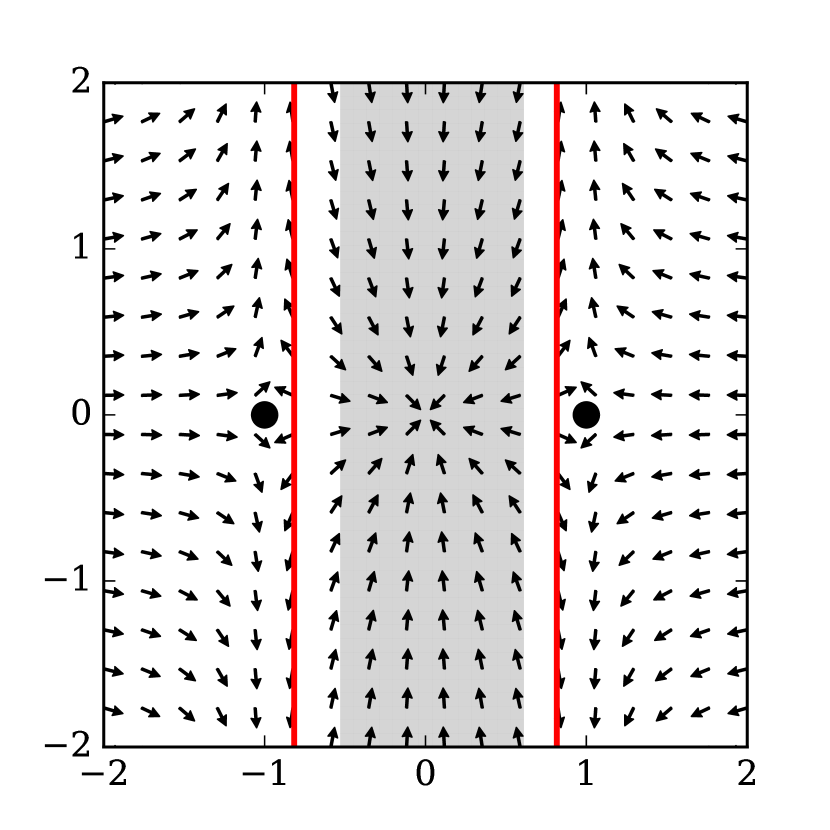
(a) $\alpha=2$

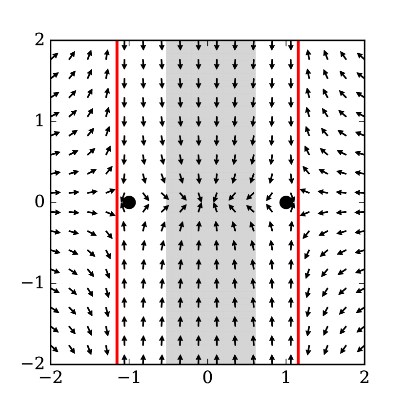
(b) $\alpha=6$

Figure 1: $E(x,y)=(1-x^{2})^{2}+\alpha y^{2}$. This energy landscape contains a saddle at $(0,0)$, two minima at $x=\pm 1,y=0$ (black dots), and singularities at $x=\pm r_{c}$ (red line). Arrows indicate the direction of the ISD. The shaded region is the index-1 region where $\lambda_{1}<0<\lambda_{2}$.

This example shows the importance of singularities for the ISD. The GAD, due to the lag in the evolution of $v$, does not adapt instantaneously to the discontinuity of the first eigenvector. Instead one expects that it will oscillate back and forth near a singularity, at least for $\varepsilon$ sufficiently small.

Neither of the two examples we discussed here is generic: in the 1D example (5) both ISD and GAD reduce to gradient ascent, while in the 2D example (6) the set of singularities is a line, whereas we expect point singularities; we will discuss this in detail in § 3.1.

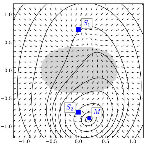
Figure 2: $E(x,y)=(x^{2}+y^{2})^{2}+x^{2}-y^{2}-x+y$, a coercive energy functional with a minimum at $M$, an attractive singularity at $S_{1}$ and a repulsive singularity at $S_{2}$. The shaded area is the index-1 region. The arrows indicate the direction of the ISD. The black lines are contour lines of $E$. The ISD remains trapped in this energy well, and trajectories converge to $S_{1}$. This example shows, in particular, that an index-1 region is insufficient to guarantee even the existence of a saddle.

1.4 New Results: basin of attraction

The basin of convergence of the saddle $\{(x,y),|x|\leq\min(1,r_{c})\}$ for (6) is fairly large and in particular includes the index-1 region $\{(x,y),|x|\leq\frac{1}{\sqrt{3}}\}$ where the first two eigenvalues $\lambda_{1}(x)$ and $\lambda_{2}(x)$ of $\nabla^{2}E(x)$ satisfy $\lambda_{1}(x)<0<\lambda_{2}(x)$. This and other examples motivate the intuition that, when started in such an index-1 region, the ISD and GAD will converge to a saddle.

Our results in Section 2 formalizes this intuition but with an added assumption: we prove in Theorem 2 that the ISD converges to a saddle if it is started in a an index-1 region $\Omega$ that is a connected component of a sublevel set for $\|\nabla E\|$. In Theorem 2 the same result is proven for the GAD, under the additional requirement that $\|v(0)-v_{1}(x(0))\|$ and $\varepsilon$ are sufficiently small.

These results give some credence to the importance of index-1 regions, but only guarantee convergence under a (strong) additional hypothesis. We show in Figure 2 an index-1 region with no saddles inside, demonstrating the importance of this additional hypothesis.

1.5 New Results: singularities and quasi-periodic orbits

Let $E\in C^{2}(\mathbb{R}^{N})$ and, for $x\in\mathbb{R}^{N}$, let $\lambda_{1}(x)\leq\lambda_{2}(x)$ denote the two first eigenvalues of $\nabla^{2}E(x)$ and $v_{1}(x),v_{2}(x)$ the associated eigenvectors. The set at which eigenvalues cross is the set of singularities

$$\mathcal{S}\mathrel{\mathop{\mathchar 58\relax}}=\big{\{}x\in\mathbb{R}^{N}\,|\,\lambda_{1}(x)=\lambda_{2}(x)\big{\}}.$$

Note that $v_{1}(x)$ is well-defined only for $x\in\mathbb{R}^{N}\setminus\mathcal{S}$. Accordingly, the ISD is defined only away from $\mathcal{S}$.

In Section 3, we study the local structure of singularities in 2D. We first show that, unlike in § 1.3, singularities are generically isolated, and stable with respect to perturbations of the energy functional. We then examine the ISD around isolated singularities, in particular classifying attractive singularities such as $S_{1}$ in Figure 2, which give rise to finite-time blow-up of the ISD.

For such attractive singularities, the GAD does not have time to adapt to the rapid fluctuations of $v_{1}(x)$ and oscillates around the singularity. For $\varepsilon$ small, we prove in special cases that the resulting behavior for the GAD is a stable annulus of radius $O(\varepsilon)$ and of width $O(\varepsilon^{2})$ around the singularity. We call such a behavior “quasi-periodic”. Our main result is Theorem 8, which generalizes this to the multi-dimensional setting and proves stability with respect to arbitrary small perturbations of the energy functional $E$.

1.6 Notation

We call $N\geq 1$ the dimension of the ambient space, and $(e_{i})_{1\leq i\leq N}$ the vectors of the canonical basis. For a matrix $M$, we write $\|M\|_{\text{op}}=\sup_{x\in S_{1}}\|Mx\|$ its operator norm, where $S_{1}$ denotes the unit sphere in $\mathbb{R}^{N}$. In our notation, $I$ is the identity matrix and scalars may be interpreted as matrices. Matrix inequalities are to be understood in the sense of symmetric matrices: thus, for instance, when $\lambda\in\mathbb{R}$, $M\geq\lambda$ and $M-\lambda\geq 0$ both mean that $\left\langle x,Mx\right\rangle\geq\lambda\|x\|^{2}$ for all $x\in\mathbb{R}^{N}$. When $A$ is a third-order tensor and $u,v,w\in\mathbb{R}^{N}$, we write $A[u]$ for the contracted matrix $(A[u])_{ij}=\sum_{k=1}^{N}A_{ijk}u_{k}$, and similarly $A[u,v]$ and $A[u,v,w]$ for the contracted vector and scalar.

$E$ will always denote an energy functional defined on $\mathbb{R}^{N}$. We will write $\nabla^{k}E(x)$ for the $k$-th-order tensor of derivatives at $x$. $\lambda_{i}(x)$ and $v_{i}(x)$ refer to the $i$-th eigenvalue and eigenvector (whenever this makes sense) of $\nabla^{2}E(x)$.

A $2\times 2$ matrix representing a rotation of angle $\omega$ will be denoted by $R_{\omega}$.

2 Region of attraction

2.1 Idealized dynamics

We first consider the ISD (3), and prove local convergence around non-degenerate index-1 saddles.

Lemma 1.

(a) Let $E\in C^{3}(\mathbb{R}^{N})$ and $\lambda_{1}(x_{*})<\lambda_{2}(x_{*})$ for some $x_{*}\in\mathbb{R}^{N}$, then

$$F_{\rm ISD}(x)\mathrel{\mathop{\mathchar 58\relax}}=-(I-2v_{1}(x)\otimes v_{1}(x))\nabla E(x)$$

is $C^{1}$ in a neighborhood of $x_{*}$.

(b) If $x_{*}\in\mathbb{R}^{N}$ is an index-1 saddle, then $\nabla F_{\rm ISD}(x_{*})$ is symmetric and negative definite. In particular, $x_{*}$ is exponentially stable under the ISD (3).

Proof.

The proof of (a) follows from a straightforward perturbation argument for the spectral decomposition, given the spectral gap $\lambda_{1}<\lambda_{2}$. As part of this proof one obtains that $x\mapsto v_{1}(x)\in C^{1}$.

To prove (b), we observe that, since $\nabla E(x_{*})=0$,

$$\nabla F_{\rm ISD}(x_{*})[h] =-(I-2v_{1}\otimes v_{1})\nabla^{2}E(x_{*})[h]+2\nabla v_{1}[h]\left\langle v_{1},\nabla E(x_{*})\right\rangle+2(v_{1}\otimes\nabla v_{1}[h])\nabla E(x_{*})$$

$$=-(I-2v_{1}\otimes v_{1})\nabla^{2}E(x_{*})[h].$$

Therefore, $\nabla F_{\rm ISD}(x_{*})$, is symmetric and negative definite, which implies the result. ∎

Next we give an improved estimate on the ISD region of attraction of an index-1 saddle.

Theorem 2.

Let $E\in C^{3}(\mathbb{R}^{N})$, $L>0$ a level and let $\Omega\subset\mathbb{R}^{N}$ be a closed connected component of $\{x\in\mathbb{R}^{N}\,|\,\|\nabla E(x)\|\leq L\}$ which is bounded (and therefore compact). Suppose, further, that $\lambda_{1}(x)<0<\lambda_{2}(x)$ for all $x\in\Omega$.

Then, for all $x_{0}\in\Omega$, the ISD (3) with initial condition $x(0)=x_{0}$ admits a unique global solution $x\in C^{1}([0,\infty);\Omega)$. Moreover, there exist an index-1 saddle $x_{*}\in\Omega$ and constants $K,c>0$ such that

$$\|x(t)-x_{*}\|\leq Ke^{-ct}.$$

Proof.

The result is based on the observation that, if $x\in C^{1}([0,T])$ solves the ISD (3), then for $0<t<T$,

$$\frac{d}{dt}\|\nabla E(x)\|^{2} =2\left\langle\frac{d}{dt}\nabla E(x),\nabla E(x)\right\rangle$$

$$=2\left\langle\nabla^{2}E(x)\dot{x},\nabla E(x)\right\rangle$$

$$=-2\left\langle\nabla E(x),\;\nabla^{2}E(x)(I-2v\otimes v)\nabla E(x)\right\rangle$$

$$\leq-2\min(-\lambda_{1},\lambda_{2})\|\nabla E(x)\|^{2}.$$

It follows that $\Omega$ is a stable region for the ISD. Since $\Omega$ is bounded and $\mathcal{S}\cap\Omega=\emptyset$, if $x(0)\in\Omega$, then (3) has a global solution $x\in C^{1}([0,\infty);\Omega)$.

Because $\Omega$ is compact, $\inf_{x\in\Omega}-2\min(-\lambda_{1},\lambda_{2})>0$. It follows that $\nabla E(x(t))\to 0$ with an exponential rate. Again by compactness, there exists $x_{*}\in\Omega$ and a subsequence $t_{n}\uparrow\infty$ such that $x(t_{n})\to x_{*}$. Since $\nabla E(x(t))\to 0$, we deduce $\nabla E(x_{*})=0$. Since $\lambda_{1}(x_{*})<0<\lambda_{2}(x_{*})$ it follows that $x_{*}$ is an index-1 saddle.

Since we have now shown that, for some $t>0$, $x(t)$ will be arbitrarily close to $x_{*}$, the exponential convergence rate follows from Lemma 1. ∎

2.2 Gentlest Ascent Dynamics

The analogue of Theorem 2 for the GAD (4) requires that the relaxation of the rotation is sufficiently fast and that the initial orientation $v(0)$ is close to optimal.

Theorem 3.

Assume the same prerequisites as Theorem 2.

Then, for $\varepsilon,\delta>0$ sufficiently small, the GAD (4) with any initial condition $x(0)=x_{0}\in{\rm int}(\Omega)$ and $v_{0}\in S_{1}$ such that $\|v(0)-v_{1}(x_{0})\|<\delta$ admits a unique global solution $(x,v)\in C^{1}([0,\infty);\Omega\times S_{1})$. Moreover, there exists an index-1 saddle $x_{*}\in\Omega$, and constants $K,c>0$ such that

$$\|x(t)-x_{*}\|+\|v(t)-v_{1}(x_{*})\|\leq Ke^{-ct}.$$

The proof of this result, which is more technical but at its core follows the same idea as Theorem 2, can be found in Appendix A. The additional ingredient is to control $\|v(t)-v_{1}(x(t))\|$, using smallness of $\varepsilon$ and the separation of the eigenvalues $\lambda_{1}<0<\lambda_{2}$ in $\Omega$.

2.3 An example of global convergence and benchmark problem

An immediate corollary of Theorem 3 is the following result.

Corollary 4.

Suppose that $E\in C^{3}(\mathbb{R}^{N})$ has the properties

$$\lambda_{1}(x)<0<\lambda_{2}(x)\qquad\forall x\in\mathbb{R}^{N},$$

$$\|\nabla E(x)\|\to\infty\qquad\text{as }|x|\to\infty.$$

Then, for every $r>0$ there exists $\varepsilon_{r},\delta_{r}>0$ such that the $\varepsilon$-GAD (4) with $\varepsilon\leq\varepsilon_{r}$ and initial conditions satisfying $\|x(0)\|\leq r$ and $\|v(0)-v_{1}(x(0))\|\leq\delta_{r}$ has a unique global solution $(x(t),v(t))$ which converges to an index-1 saddle.

We mention this result as it establishes a simplified yet still non-trivial situation, somewhat analogous to convex objectives in optimization, in which there is a realistic chance to develop a rigorous global convergence theory for practical saddle search methods that involve adaptive step size selection and choice of rotation accuracy. Work in this direction would generate ideas that strengthen the robustness and efficiency of existing saddle search methods more generally.

3 Singularities and (quasi-)periodic orbits

We now classify the singularities $\mathcal{S}$ for the ISD (3) in 2D, exhibit finite-time blow-up of the ISD and (quasi-)periodic solutions of the GAD.

3.1 Isolated singularities and the discriminant

Recall that the set of singularities for the ISD is denoted by $\mathcal{S}=\{x\in\mathbb{R}^{2}\,|\,\lambda_{1}(x)=\lambda_{2}(x)\}$. The ISD is defined on $\mathbb{R}^{2}\setminus\mathcal{S}$.

Since symmetric matrices with repeated eigenvalues are a subset of codimension 2 of the set of symmetric matrices, one can expect that $\mathcal{S}$ contains isolated points. This phenomenon is sometimes known as the Von Neumann-Wigner no-crossing rule [11].

This is particularly easy to see in dimension 2, because the only $2\times 2$ matrices with repeated eigenvalues are multiples of the identity, and therefore are a 1-dimensional subspace of the 3-dimensional space of $2\times 2$ symmetric matrices. To transfer this to the set $\mathcal{S}$, we first note that a point $x\in\mathbb{R}^{2}$ is a singularity if and only if

$$\left\langle e_{1},\nabla^{2}E(x)e_{1}\right\rangle =\left\langle e_{2},\nabla^{2}E(x)e_{2}\right\rangle,$$

$$\left\langle e_{2},\nabla^{2}E(x)e_{1}\right\rangle =0.$$

Writing this system of equations in the form $F(x)=0$, if the Jacobian $\nabla F(0)$ is invertible, then the singularity is isolated.

For $i,j,k=1,2$ we define

$$E_{ijk} =\nabla^{3}E(0)[e_{i},e_{j},e_{k}],\qquad\Delta=(E_{111}E_{122}+E_{112}E_{222})-E_{112}^{2}+E_{122}^{2},$$

then we can compute

$${\nabla F}(0) =\begin{pmatrix}E_{111}-E_{122}&E_{112}-E_{222}\\ E_{112}&E_{122}\\ \end{pmatrix}\qquad\text{and}\qquad\det(\nabla F(0))=\Delta.$$

If $\Delta\neq 0$ (which we expect generically) then the singularity is isolated. By the implicit function theorem, this also implies that such a singularity is stable with respect to small perturbations of the energy functional (see Lemma 9 for more details).

Note that this it not the case for the example $E(x,y)=(1-x^{2})^{2}+\alpha y^{2}$ of Section 1.3, which has a line of singularities on which $\Delta=0$. This is due to the special form of the function, where the hessian is constant along vertical lines. This behavior is not generic, and under most perturbations the singularity set $\mathcal{S}$ will change to a discrete set (this statement can be proven using the transversality theorem).

3.2 Formal expansion of the ISD and GAD near a singularity

We consider the ISD and GAD dynamics in the neighborhood of a singularity situated at the origin. In the following, we assume $\Delta\neq 0$, so that the singularity is isolated.

Let $\lambda\mathrel{\mathop{\mathchar 58\relax}}=\lambda_{1}(0)=\lambda_{2}(0)$, then expanding $E$ about $0$ yields

$$\nabla E(x) =\nabla E(0)+\lambda x+O(\|x\|^{2}),$$

$$\nabla^{2}E(x) =\lambda I+\nabla^{3}E(0)[x]+O(\|x\|^{2}).$$

Inserting these expansions into the GAD (4) yields

$$\dot{x} =-(I-2v\otimes v)\nabla E(0)+O(\|x\|),$$

$$\varepsilon^{2}\dot{v} =-(I-v\otimes v)\nabla^{3}E(0)[x,v]+O(\|x\|^{2}),$$

and dropping the higher-order terms we obtain the leading-order GAD

$$\begin{split}\dot{x}&=-(I-2v\otimes v)\nabla E(0),\\ \varepsilon^{2}\dot{v}&=-(I-v\otimes v)\nabla^{3}E(0)[x,v].\end{split}$$ (7)

Since $\Delta\neq 0$, $v_{1}(x)$ is well-defined in $B_{r}(0)\setminus\{0\}$ for some $r>0$. To leading order, $v_{1}(x)$ is given by

$$v_{1}(x)=w_{1}(x)+O(\|x\|),$$

where $w_{1}$ is the eigenvector corresponding to the first eigenvalue of $\nabla^{3}E(0)[x]$. Inserting the expansions for $\nabla^{2}E$ and $v_{1}$ into the ISD yields

$$\dot{x}=-(I-2w_{1}(x)\otimes w_{1}(x))\nabla E(0)+O(\|x\|),$$

and dropping again the $O(\|x\|)$ term we arrive at the leading-order ISD

$$\dot{x}=-(I-2w_{1}(x)\otimes w_{1}(x))\nabla E(0).$$ (8)

Next, we rewrite the leading-order GAD and ISD in a more convenient format. If $v=(\cos\phi,\sin\phi)\in S_{1},$ then we define

$$\bar{v}\mathrel{\mathop{\mathchar 58\relax}}=\big{(}\cos(2\phi),\sin(2\phi)\big{)}.$$ (9)

Furthermore, we define the matrix

$$A\mathrel{\mathop{\mathchar 58\relax}}=\begin{pmatrix}\frac{E_{111}-E_{122}}{2}&\frac{E_{112}-E_{222}}{2}\\ E_{112}&E_{122}\end{pmatrix},$$ (10)

which coincides with $\nabla F(0)$, up to the scaling of the first row. In particular, $\det A=\frac{1}{2}\Delta$.

Lemma 5.

Suppose that $\nabla E(0)=(\cos\alpha,\sin\alpha)$, then the leading-order GAD (7) and ISD (8) are, respectively, given by

$$\begin{split}\dot{x}&=R_{-\alpha}\bar{v},\\ \varepsilon^{2}\dot{\bar{v}}&=-2\big{\langle}R_{\pi/2}\bar{v},Ax\big{\rangle}R_{\pi/2}\bar{v}\end{split}$$ (11)

and

$$\dot{x}=-\frac{R_{-\alpha}Ax}{\|Ax\|}.$$ (12)

Proof.

For $y=(a,b)\in\mathbb{R}^{2}$, we define the matrix

$$\operatorname{Q}_{y} =\begin{pmatrix}a&b\\ b&-a\end{pmatrix}.$$

Geometrically, if $\|y\|=1$, then $\operatorname{Q}_{y}$ describes a reflection with respect to the line whose directing angle is half that of $y$. Accordingly, for $v\in S_{1}$,

$$I-2v\otimes v =-\operatorname{Q}_{\bar{v}},$$ (13)

and hence the evolution of $x$ in the leading-order GAD equation (7) reduces to

$$\dot{x} =\operatorname{Q}_{\bar{v}}R_{\alpha}e_{1}=R_{-\alpha}\operatorname{Q}_{\bar{v}}e_{1}=R_{-\alpha}\bar{v},$$

which establishes the first equation in (11).

To derive the second equation in (11), subtracting the average of the diagonal entries of $\nabla^{3}E(0)[x]$ yields

$$\nabla^{3}E(0)[x]=\begin{pmatrix}E_{111}x_{1}+E_{112}x_{2}&E_{112}x_{1}+E_{122}x_{2}\\ E_{112}x_{1}+E_{122}x_{2}&E_{122}x_{1}+E_{222}x_{2}\end{pmatrix}=c(x)I+\operatorname{Q}_{Ax},$$

for some $c(x)\in\mathbb{R}$. Together with $I-v\otimes v=R_{\pi/2}v\otimes R_{\pi/2}v$ and $\langle R_{\pi/2}v,cIv\rangle=c\langle R_{\pi/2}v,v\rangle=0$ this observation implies

$$\varepsilon^{2}\dot{v} =-\big{\langle}R_{\pi/2}v,\big{[}cI+\operatorname{Q}_{Ax}]v\big{\rangle}R_{\pi/2}v=-\left\langle R_{\pi/2}v,\operatorname{Q}_{Ax}v\right\rangle R_{\pi/2}v.$$

Writing $Ax=(a,b)$ and $v=(\cos\phi,\sin\phi)$, we obtain

$$\left\langle v,\operatorname{Q}_{Ax}v\right\rangle =-b\big{(}\cos^{2}\phi-\sin^{2}\phi\big{)}+2a\cos\phi\sin\phi$$

$$=-b\cos(2\phi)+a\sin(2\phi)=\big{\langle}R_{\pi/2}\bar{v},Ax\big{\rangle}$$

and thus arrive at

$$\varepsilon^{2}\dot{v}=-\big{\langle}R_{\pi/2}\bar{v},Ax\big{\rangle}R_{\pi/2}v.$$

Using the observations

$$\dot{v}=\dot{\phi}R_{\pi/2}v\qquad\text{and}\qquad\dot{\bar{v}}=\dot{\phi}2R_{\pi/2}\bar{v}$$

immediately yields the second equation in (11).

Finally, to obtain (12) we first observe that the stationary points for the $\bar{v}$ equation of unit norm are $\bar{w}^{\pm}=\pm{Ax}/{\|Ax\|}$, the stable one being $\bar{w}^{-}=-Ax/\|Ax\|$ (corresponding to $v$ being the lowest eigenvector of $\operatorname{Q}_{Ax}$ and therefore $\nabla^{3}E(0)[x]$). Applying (13) we obtain

$$\dot{x}=\operatorname{Q}_{\bar{w}^{-}}R_{\alpha}e_{1}=R_{-\alpha}\bar{w}^{-}=-\frac{R_{-\alpha}Ax}{\|Ax\|}.\qed$$

3.3 Finite-time blow-up of the ISD near singularities

We assume, without loss of generality, that $\|\nabla E(0)\|=1$. Then it follows from Lemma 5 that the ISD is given by

$$\dot{x}=-\frac{R_{-\alpha}Ax}{\|Ax\|}+O(\|x\|),$$

where $A$ is given by (10). Thus, starting sufficiently close to the origin, we can study the ISD using the tools of linear stability. Observe first that

$$\det(R_{-\alpha}A)=\det A=\frac{\Delta}{2}.$$

If $\Delta>0$ then $R_{-\alpha}A$ either has two real eigenvalues with the same sign or it has a pair of complex conjugate eigenvalues. This results in a singularity that is either attractive, repulsive or a center (see Figure 3(a), 3(b) and 3(c) respectively). If $\Delta<0$, $R_{-\alpha}A$ has two real eigenvalues of opposite sign and hence the origin will exhibit saddle-like behavior; cf. Figure 3(d).

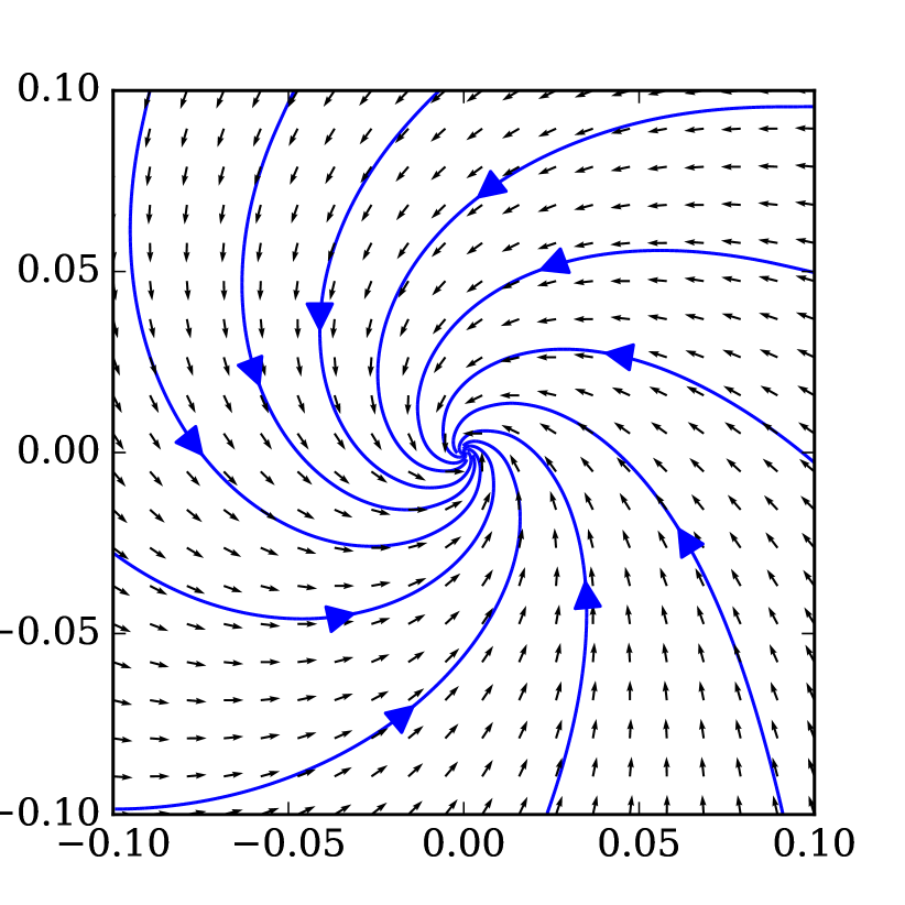
(a) Stable spiral: $s=1,\alpha=\pi/4,\Delta=-2$

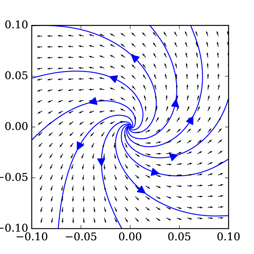
(b) Unstable spiral: $s=1,\alpha=3\pi/4,\Delta=-2$

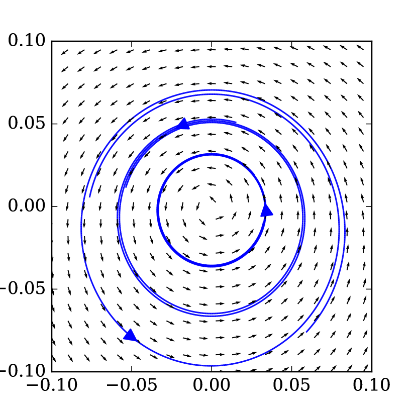
(c) Center: $s=1,\alpha=\pi/2,\Delta=-2$.

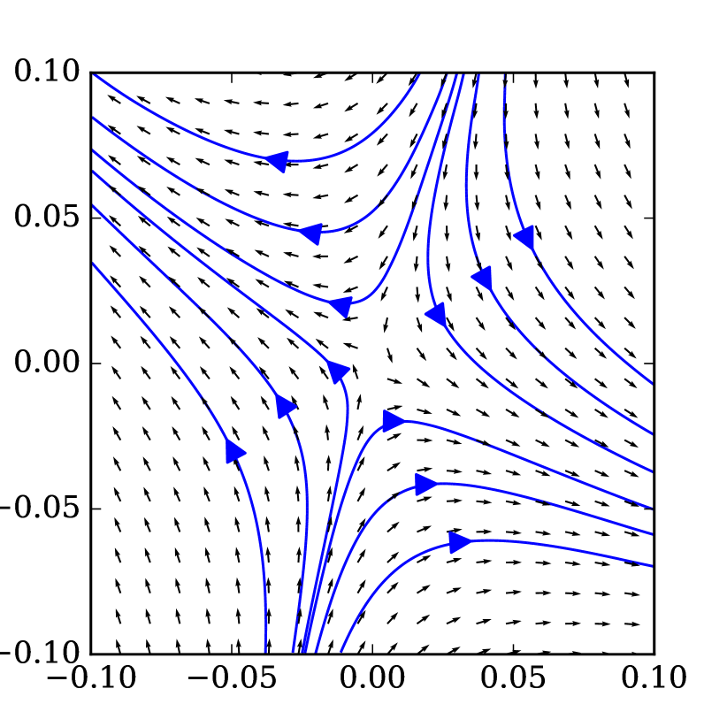
(d) Saddle: $s=-1,\alpha=\pi,\Delta=4$

Figure 3: ISD phase planes near a singularity at $0$. The energy functional is $E(x)=\cos\alpha x_{1}+\sin\alpha x_{2}+\frac{1}{2}(x_{1}^{2}+x_{2}^{2})+\frac{1}{2}(sx_{1}^{3}+x_{1}x_{2}^{2})$.

We are specifically interested in attractive singularities such as the one in Figure 3(a). In this context, we prove the following proposition:

Proposition 6.

Suppose that $0\in\mathcal{S}$ is a singularity such that $\Delta>0$ and that $R_{-\alpha}A$ has two eigenvalues (counting multiplicity) with positive real part. Then, for $\|x(0)\|\neq 0$ sufficiently small the corresponding maximal solution $x\in C^{1}([0,T_{*}))$ of (3) has blow-up time $T_{*}<\infty$ and $x(t)\to 0$ as $t\to T_{*}$.

Proof.

We have shown in Lemma 5 that the ISD can be written in the form

$$\dot{x} =\frac{1}{\|Bx\|}\left(-Bx+g(x)\right),$$

where $B=R_{-\alpha}A$ has eigenvalues with positive real part, $\|g(x)\|\leq C\|x\|^{2}$ for $x$ in a neighborhood of the origin, and $C>0$ a constant. According to standard ODE theory, there is a maximal solution $x(t)$ in an interval $[0,T_{*})$. Assuming $T_{*}=\infty$, we will obtain a contradiction by showing that $x(t)=0$ for some finite $t$.

Diagonalizing $B$ (or taking its Jordan normal form), there exists an invertible $P\in\mathbb{R}^{2\times 2}$ such that $B=PDP^{-1}$, with $D$ of one of the following three forms:

$$D=\begin{pmatrix}\lambda_{r}&-\lambda_{i}\\ \lambda_{i}&\lambda_{r}\end{pmatrix},\qquad D=\begin{pmatrix}\lambda_{1}&0\\ 0&\lambda_{2}\end{pmatrix},\qquad\text{or}\qquad D=\begin{pmatrix}\lambda&\varepsilon\\ 0&\lambda\end{pmatrix},$$

where $\varepsilon$ may be chosen arbitrarily small. In all cases, by the hypothesis that $B$ has eigenvalues with positive real parts, $D$ is invertible, and there exists $\mu>0$ such that $\left\langle x,Dx\right\rangle\geq\mu\|x\|^{2}$ for all $x\in\mathbb{R}^{2}$.

Setting $x=Py$, we obtain

$$\dot{y} =-\frac{Ry+g(Py)}{\|PRy\|}$$

and therefore

$$\frac{1}{2}\frac{d}{dt}\|y\|^{2} \leq\frac{-\langle Dy,y\rangle+g(Py)}{\|PDy\|}\leq-C_{1}\|y\|+C_{2}\|y\|^{2},$$

where $C_{1}=\frac{\mu}{\|R\|\|P\|},C_{2}=C\|P^{-1}\|\|R^{-1}\|\|P\|^{2}$, for $y$ in a neighborhood of zero. It follows that, when $\|x(0)\|$ is sufficiently small, then $\|y\|^{2}$ is decreasing and reaches zero in finite time. ∎

Proposition 6 demonstrates how the ISD, a seemingly ideal dynamical system to compute saddle points can be attracted into point singularities and thus gives a further example of how the global convergence of the ISD fails. Next, we examine the consequences of this result for the GAD.

3.4 The isotropic case

The GAD (11) is a nonlinear dynamical system of dimension 3 (two dimensions for $x$, one for $\bar{v}$), who are known to exhibit complex (e.g. chaotic) behavior. In the setting of Proposition 6, we expect that “most” solutions of the GAD converge to a limit cycle. Numerical experiments strongly support this claim, but indicate that the limit cycles can be complex; see Figure 4.

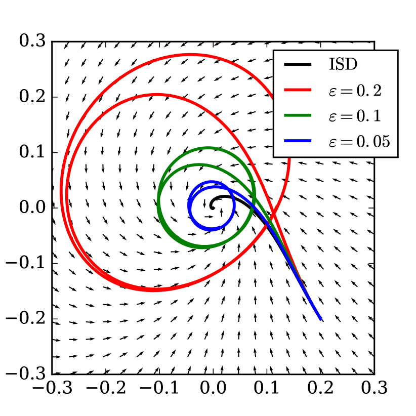
(a) ISD and GAD for $E(x)=\cos\alpha x_{1}+\sin\alpha x_{2}+\frac{1}{2}(x_{1}^{2}+x_{2}^{2})+\frac{1}{2}(x_{1}^{3}+x_{1}x_{2}^{2})$, $\alpha=\pi/4$; cf. Sections 3.4 and 3.5.
 

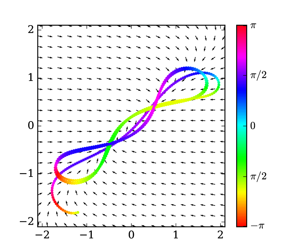
(b) Leading order GAD (11) in a non-isotropic case: $\alpha=-1,A=\begin{pmatrix}-0.3&0.4\\ -0.4&0.3\end{pmatrix}$, which has singular values $0.7$ and $0.1$. The color corresponds to the phase of $\bar{v}$.

Figure 4: Leading order ISD and GAD in an isotropic (left) and anisotropic (right) case.

We now seek to rigorously establish the existence of (quasi-)periodic behavior of the GAD, at least in special cases. To that end we write

$$A=R_{s}DR_{t},\qquad\text{where }R_{s},R_{t}\in{\rm SO}(2)\quad\text{and }D={\rm diag}(d_{1},d_{2}),$$

and we recall that $d_{1}d_{2}=\det D=\det A=\Delta/2>0$, that is, $d_{1},d_{2}$ have the same sign. Since $R_{s},R_{t},R_{-\alpha},R_{\pi/2}$ commute, under the substitution $y=R_{t}x,\bar{w}=R_{-s}\bar{v}$, the leading-order GAD becomes

$$\dot{y} =R_{s-t-\alpha}\bar{w},$$

$$\varepsilon^{2}\dot{\bar{w}} =-2\langle R_{\pi/2}\bar{w},Dy\rangle R_{\pi/2}\bar{w}.$$

From Figure 4 we observe that a complex limit cycle can occur in the anisotropic case $d_{1}\neq d_{2}$, while the behavior when $d_{1}=d_{2}$ is much simpler. In order to get a tractable system, we restrict ourselves in the following to the isotropic case $d_{1}=d_{2}$, where we can use polar coordinates to perform a stability analysis. Note that this corresponds to imposing that $A$ is a multiple of a rotation matrix: $A_{11}=A_{22}$, $A_{12}=-A_{21}$. This is equivalent to the condition $E_{111}=3E_{122},E_{222}=3E_{112}$, i.e. the cubic terms are of the form $ax_{1}^{3}+bx_{1}^{2}x_{2}+ax_{1}x_{2}^{2}+bx_{2}^{3}$, for any $a,b\in\mathbb{R}$.

Under this hypothesis, $A=dR_{t}$ for some scalars $d>0,t\in\mathbb{R}$. Under the transformations $x\leadsto R_{t}x,\varepsilon^{2}\leadsto\varepsilon^{2}/d,\alpha\leadsto\alpha-t$, the leading order GAD equations (11) become

$$\begin{split}\dot{x}&=R_{-\alpha}\bar{v}\\ \varepsilon^{2}\dot{\bar{v}}&=-2\left\langle R_{\pi/2}\bar{v},x\right\rangle R_{\pi/2}\bar{v}.\end{split}$$ (14)

Thus, up to a rescaling of $\varepsilon$, a rotation of $x$ and a shift in $\alpha$ (rotation of $\nabla E(0)$), restricting to isotropic matrices is equivalent to restricting to $A=I$, which corresponds to

$$E_{111}=3,\quad E_{112}=0,\quad E_{122}=1,\quad E_{222}=0,$$

or

$$E(x)=\cos\alpha x_{1}+\sin\alpha x_{2}+\frac{\lambda}{2}(x_{1}^{2}+x_{2}^{2})+\frac{1}{2}(x_{1}^{3}+x_{1}x_{2}^{2})+O(\|x\|^{4}).$$ (15)

We consider this case in the sequel, as well as the restriction $\cos\alpha>0$, which ensures that $R_{-\alpha}$ has eigenvalues with positive real part and therefore that the ISD converges to zero.

3.5 Explicit solutions of the leading-order GAD in the attractive isotropic case

We now produce an explicit solution of the leading-order isotropic GAD (14), which makes precise the intuition that delayed orientation relaxation of the GAD balances the blow-up of the ISD and thus leads to periodic orbits.

On substituting polar coordinates

$$x=r(\cos\theta,\sin\theta),\qquad v=(\cos\phi,\sin\phi)\qquad\text{and hence}\qquad\bar{v}=(\cos 2\phi,\sin 2\phi)$$

in (14) we obtain a set of three coupled ODEs for $r,\theta$ and $\phi$:

$$\begin{split}\dot{r}&=\cos(2\phi-\alpha-\theta)\\ r\dot{\theta}&=\sin(2\phi-\alpha-\theta)\\ \varepsilon^{2}\dot{\phi}&=r\sin(2\phi-\theta).\end{split}$$ (16)

We now analyze the behavior of this set of equations for $\varepsilon\ll 1$. This corresponds to an adiabatic limit where the evolution of $v$ is fast enough to relax instantly to its first eigenvector, so that the dynamics mimics closely the ISD. However, this is counterbalanced by the fact that the dynamics for $v$ becomes slow as $r\to 0$.

The $r$ dynamics takes place at a timescale $1$, the $\theta$ dynamics at a timescale $r$, and the $\phi$ dynamics at a timescale $\frac{\varepsilon^{2}}{r}$. The adiabatic approximation of fast relaxation for $v$ (the ISD) is valid when $\frac{\varepsilon^{2}}{r}\ll r$, or $r\gg\varepsilon$. In this scaling we recover the ISD (12). One the other hand, when $r\ll\varepsilon$, then $\theta$ relaxes to a stable equilibrium $2\phi-\alpha-\theta=2k\pi,k\in\mathbb{Z}$, in which case we obtain $\dot{r}=+1$. Therefore we may expect that for $r\gg\varepsilon$, $r$ decreases, while for $r\ll\varepsilon$, $r$ increases.

We now examine the intermediate scaling $r\sim\varepsilon$. Rescaling $r=\varepsilon r^{\prime}$ we obtain

$$\varepsilon\dot{r}^{\prime} =\cos(2\phi-\alpha-\theta)$$

$$\varepsilon r^{\prime}\dot{\theta} =\sin(2\phi-\alpha-\theta)$$

$$\varepsilon\dot{\phi} =r^{\prime}\sin(2\phi-\theta).$$

All variables now evolve at the same characteristic timescale $\varepsilon$, hence we rescale $t=\varepsilon t^{\prime}$. For the sake of simplicity of presentation we drop the primes to obtain the system

$$\begin{split}\dot{r}&=\cos(2\phi-\alpha-\theta)\\ r\dot{\theta}&=\sin(2\phi-\alpha-\theta)\\ \dot{\phi}&=r\sin(2\phi-\theta),\end{split}$$ (17)

which describes the evolution (16) on time and space scales of order $\varepsilon$.

We observe that the evolution of (17) does not depend on $\theta$ and $\phi$ individually, but only on $\omega=2\phi-\theta$. Keeping only the variables of interest, $r$ and $\omega$, we arrive at the 2-dimensional system

$$\begin{split}\dot{r}&=\cos(\omega-\alpha)\\ \dot{\omega}&=2r\sin\omega-\frac{1}{r}\sin(\omega-\alpha).\end{split}$$ (18)

Since $\cos\alpha>0$, (18) has two fixed points, with associated stability matrix $J^{\pm}$,

$$r_{0}=\sqrt{\frac{1}{2\cos\alpha}},\qquad\omega_{0}^{\pm}=\alpha\pm\frac{\pi}{2},\qquad J^{\pm}=\begin{pmatrix}0&\mp 1\\ \pm 4\cos\alpha&\mp\frac{2\sin\alpha}{\sqrt{2\cos\alpha}}\end{pmatrix}.$$ (19)

The determinant of $J^{\pm}$ is positive. The eigenvalues are either complex conjugate or both real; in both cases their real part is of the same sign as the trace,

$$\text{tr}J^{\pm}=\mp\frac{2\sin\alpha}{\sqrt{2\cos\alpha}}.$$

If $\sin\alpha>0$, then $(r_{0},\omega_{0}^{+})$ is stable, whereas if $\sin\alpha<0$, then $(r_{0},\omega_{0}^{-})$ is stable. The case $\sin\alpha=0$ cannot be decided from linear stability, and so we exclude it in our analysis.

In real variables, the resulting behavior is that the system stabilizes in a periodic orbit at $r_{0}=\varepsilon\sqrt{\frac{1}{2\cos\alpha}}$. $\theta$ evolves twice at fast as $\phi$, so that $\omega=2\phi-\theta$ stays constant at $\omega^{\pm}=\alpha\pm\frac{\pi}{2}$. Thus we have established the following result.

Lemma 7.

If $\cos\alpha>0,\sin\alpha\neq 0$, then the projection (18) of the leading order isotropic GAD admits a stable circular orbit of radius

$$r =\frac{\varepsilon}{\sqrt{2\cos\alpha}}.$$

In the next section, we will show that this behavior survives to a threefold generalization: the re-introduction of the neglected higher-order terms, perturbations of the energy functional, as well as dimension $N>2$.

3.6 Quasi-periodic solutions of GAD

The computation of Section 3.5 suggests that the GAD for the energy functional

$$E(x_{1},x_{2})=(\cos\alpha x_{1}+\sin\alpha x_{2})+\frac{\lambda}{2}(x_{1}^{2}+x_{2}^{2})+\frac{1}{2}(x_{1}^{3}+x_{1}x_{2}^{2})$$ (20)

has nearly periodic trajectories near the origin when $\alpha\in(-\pi/2,0)\cup(0,\pi/2)$. Any third-order term of the form $ax_{1}^{3}+bx_{1}^{2}x_{2}+ax_{1}x_{2}^{2}+bx_{2}^{3}$ for $a,b\in\mathbb{R}$ reduces to (20) upon a suitable change of variables. We will now rigorously prove the existence of quasi-periodic behavior in the multidimensional and perturbed case. We split an $N$-dimensional state space $V=\mathbb{R}^{N}$ into two components $V=V_{\rm s}\oplus V_{\rm c}$: a two-dimensional subspace $V_{\rm s}$ (singular) on which the dynamics is the same as in the 2D case, and an $(N-2)$-dimensional subspace $V_{\rm c}$ (converging) on which the GAD dynamics converges to zero. Let $I=\{1,\dots,N\}$, $I_{\rm s}=\{1,2\}$ and $I_{\rm c}=\{3,\dots,N\}$ be the corresponding set of indices and, for $x\in\mathbb{R}^{N},x_{\rm s}=(x_{1},x_{2},0,\dots,0)\in V_{\rm s}$ and $x_{\rm c}=(0,0,x_{3},\dots,x_{N})\in V_{\rm s}$.

We consider a functional $E=E^{0}$ of the form,

$$\begin{split}E^{0}(x)&=(\cos\alpha^{0}x_{1}+\sin\alpha^{0}x_{2})+\frac{\lambda^{0}}{2}(x_{1}^{2}+x_{2}^{2})+\frac{1}{2}(x_{1}^{3}+x_{1}x_{2}^{2})\\ &\qquad+\frac{1}{2}\sum_{i,j\in I_{\rm c}}^{N}H^{0}_{ij}x_{i}x_{j}+\frac{1}{6}\sum_{i,j,k\in I_{\rm c}}G^{0}_{ijk}x_{i}x_{j}x_{k}+O(\|x\|^{4}),\end{split}$$ (21)

where $\alpha^{0}\in(0,\pi/2)\cup(\pi/2,\pi),\lambda^{0}\in\mathbb{R}$, $H^{0}_{ij}=\nabla^{2}E^{0}(0)[e_{i},e_{j}],i,j\in I_{\rm c}$, and $G^{0}_{ijk}=\nabla^{3}E^{0}(0)[e_{i},e_{j},e_{k}]$, $i,j,k\in I$.

For $x_{\rm c}=0$, $E^{0}$ coincides with (20) to within $O(\|x\|^{4})$ and the condition on $\alpha^{0}$ are consistent with Lemma 7. We assume for the remainder that $H^{0}>\max(\lambda^{0},0)$: the requirement $H^{0}>\lambda^{0}$ ensures that $\lambda^{0}$ is indeed the lowest eigenvalue, while $H^{0}>0$ ensures that $x_{\rm c}\to 0$ as $t\to\infty$.

An example of a functional in this class, and the resulting GAD dynamics are shown in Figure 5. Our main result is the following theorem stating that the limit cycles at $r=\varepsilon/\sqrt{2\cos\alpha^{0}}$ present in the 2D leading-order GAD survive in the nonlinear, multidimensional, perturbed regime. The proof is given in Appendix B.

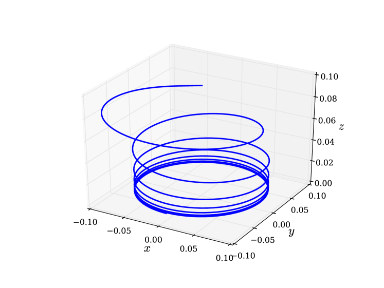
Figure 5: $E(x)=\cos\alpha x+\sin\alpha x+\frac{1}{2}(x^{2}+y^{2}+1.1z^{2})+\frac{1}{2}(x^{2}y+y^{3})+z^{3}$, $\alpha=3\pi/4$.

Theorem 8.

Let $E^{0},\Delta E\in C^{4}(\mathbb{R}^{N})$ with $E^{0}$ satisfying (21) with $H>\max(0,\lambda^{0})I$. For $\delta>0$ let $E^{\delta}\mathrel{\mathop{\mathchar 58\relax}}=E^{0}+\delta\Delta E$. Then there exist constants $\delta_{0},\varepsilon_{0},m,M>0$ such that, for all $\varepsilon<\varepsilon_{0},\delta<\delta_{0}$, the following statements hold.

1. There exists $z^{\delta}\in\mathbb{R}^{N}$ with $\|z^{\delta}\|\leq M\delta$ such that $\nabla^{2}E^{\delta}(z^{\delta})$ has repeated eigenvalues $\lambda_{1}=\lambda_{2}$ and $\nabla E^{\delta}(z^{\delta})\in{\rm span}\{e_{1},e_{2}\}$, where $e_{i}$ are the eigenvectors corresponding to $\lambda_{i}$.

2. For all $x_{0}\in\mathbb{R}^{N}$ such that $\|x_{0}-z^{\delta}\|=\varepsilon/\sqrt{2\cos\alpha^{0}}$ (cf. Lemma 7) there exists $v_{0}\in S_{1}$ such that the $\varepsilon$-GAD (4) for $E_{\delta}$ with initial conditions satisfying $\|x(0)-x_{0}\|\leq m\varepsilon(\delta+\varepsilon)$ and $\|v(0)-v_{0}\|\leq m\varepsilon(\delta+\varepsilon),{v(0)}\in S_{1}$, admits a unique solution, and

   $$\mathinner{\!\left\lvert\|x(t)-z^{\delta}\|-\frac{\varepsilon}{\sqrt{2\cos\alpha^{0}}}\right\rvert}\leq M\varepsilon(\varepsilon+\delta)\qquad\text{for all $t\geq 0$}.$$

4 Conclusion

In this paper we make two novel contributions to the theory of walker-type saddle search methods:

Region of attraction: In Section 2 we extended estimates on the region of attraction for an index-1 saddle beyond perturbative results. Our results give some credence to the widely held belief that dimer and GAD type saddle search methods converge if started in an index-1 region. But we also show through an explicit example that this is not true without some additional assumptions on the energy landscape.

We also highlight the global convergence result of Corollary 4, which we believe can provide a useful benchmark problem and testing ground towards a more comprehensive convergence theory for practical saddle search methods outside a perturbative regime.

Cycling behavior: Although it is already known from [6, 4] that the dimer and GAD methods cannot be expected to be globally convergent, the behavior identified in those references is non-generic. In Section 3 we classify explicitly the possible generic singularities and identify a new situation in which global convergence fails, which occurs in any dimension and is stable under arbitrary perturbations of the energy functional.

In particular, our results provide a large class of energy functionals for which there can be no merit function for which the ISD or GAD search directions are descent directions.

Our results illustrate how fundamentally different saddle search is from optimization, and strengthen the evidence that dimer or GAD type saddle search methods cannot be (easily) modified to obtain globally convergent schemes. Indeed it may even prove impossible to design a globally convergent walker-type saddle search method.

We speculate that this is related to the difficulty in proving the existence of saddle points in problems in calculus of variations: while the existence of minimizers follow in many cases from variational principles, the existence of saddle points is known to be more difficult, requiring sophisticated mathematical tools such as the mountain pass theorem. Such theorems are based on the minimization of functionals of paths, and as such are conceptually closer to string-of-state methods such as the nudged elastic band and string methods [8, 3]. It is to our knowledge an open question to establish the global convergence of methods from this class, but the results of the present paper suggest that it may be a more promising direction to pursue than the walker type methods.

Appendix A Proof of Theorem 3 (region of attraction for the GAD)

At a fixed configuration $x$, the dynamics on $v$ is a gradient descent for $\left\langle v,\nabla^{2}E(x)v\right\rangle$ on the sphere $S_{1}$ that ensures the local convergence of $v$ to $v_{1}$. Our strategy is to use an adiabatic argument to show that the full GAD dynamics keeps $v$ close to $v_{1}$ even when $x$ is (slowly) evolving.

Assume $\Omega$ is as in the hypotheses of this theorem. Then $\Omega$ is compact, and the minimal spectral gap $g$ of the positive-definite continuous matrix $(1-2v_{1}(x)\otimes v_{1}(x))\nabla^{2}E(x)$ satisfies

$$g =\min_{x\in\Omega}\min(-\lambda_{1}(x),\lambda_{2}(x))>0.$$

This implies that $\lambda_{2}-\lambda_{1}\geq 2g>0$ on $\Omega$. Let also

$$M=\left(\max_{x\in\Omega}\|\nabla^{2}E(x)\|_{\rm op}\right).$$

For $v\in S_{1}$, we write $P_{v}=v\otimes v$. When $v,w\in S_{1}$, then we have the following improved Cauchy-Schwarz equality

$$\left\langle v,w\right\rangle =1-\frac{1}{2}\|v-w\|^{2}$$

and bound on projectors

$$\|P_{v}-P_{w}\|_{\rm op} =\|(v-w)\otimes(v+w)\|_{\rm op}\leq 2\|v-w\|.$$

Step 1: variations of $\|\nabla E\|$.

For any $t$ such that $x(t)\in\Omega$, we compute (dropping the dependence on $x(t)$, and writing $H=\nabla^{2}E$)

$$\frac{d}{dt}\frac{1}{2}\|\nabla E\|^{2} =-\langle(I-2P_{v})H\nabla E,\nabla E\rangle$$

$$=-\langle(I-2P_{v_{1}})H\nabla E,\nabla E\rangle+\langle(P_{v}-P_{v_{1}})H\nabla E,\nabla E\rangle$$

$$\leq(-g+2M\|v-v_{1}\|)\|\nabla E\|^{2}.$$ (22)

Step 2: variations of $\|v-v_{1}\|$.

Similarly, when $x\in\Omega$, we compute

$$\frac{d}{dt}\frac{1}{2}\|v-v_{1}\|^{2} =\left\langle v-v_{1},\dot{v}-\dot{v}_{1}\right\rangle$$

$$=-\frac{1}{\varepsilon^{2}}\left\langle v-v_{1},(I-P_{v})Hv\right\rangle-\left\langle v-v_{1},\dot{v}_{1}\right\rangle.$$

Our goal is (25) below, which shows that the leading term in this expression is bounded by $-\varepsilon^{-2}g\|v-v_{1}\|^{2}$, which will pull back $v$ to $v_{1}$ when $\varepsilon$ is small enough.

We bound both terms separately. For the first term, we note that

$$(I-P_{v})Hv =(I-P_{v_{1}})H(v-v_{1})+(P_{v_{1}}-P_{v})Hv_{1}+(P_{v_{1}}-P_{v})H(v-v_{1})$$

$$=(I-P_{v_{1}})H(v-v_{1})+\lambda_{1}(v_{1}-\left\langle v,v_{1}\right\rangle v)+(P_{v_{1}}-P_{v})H(v-v_{1})$$

$$=(I-P_{v_{1}})H(v-v_{1})-\lambda_{1}\left(v-v_{1}-\frac{1}{2}\|v-v_{1}\|^{2}v\right)+(P_{v_{1}}-P_{v})H(v-v_{1}),$$

hence it follows that

$$-\varepsilon^{-2}\left\langle v-v_{1},(I-P_{v})Hv\right\rangle \leq-\varepsilon^{-2}\left\langle v-v_{1},((I-P_{v_{1}})H-\lambda_{1}I)(v-v_{1})\right\rangle$$

$$\qquad+\varepsilon^{-2}\left(\frac{1}{2}\lambda_{1}+2M\right)\|v-v_{1}\|^{3}$$

$$\leq-\varepsilon^{-2}g\|v-v_{1}\|^{2}+\varepsilon^{-2}\left(\frac{1}{2}\lambda_{1}+2M\right)\|v-v_{1}\|^{3}.$$ (23)

For the second term, standard eigenvector perturbation theory yields

$$\dot{v}_{1}=-(H-\lambda_{1})^{+}\dot{H}v_{1}=-(H-\lambda_{1})^{+}\nabla^{3}E(x)[\dot{x},v_{1}],$$

where $(H-\lambda_{1})^{+}$ is the Moore–Penrose pseudo-inverse of $H-\lambda_{1}$, defined by

$$(H-\lambda_{1})^{+}v_{1}=0\qquad\text{and}\qquad(H-\lambda_{1})^{+}v_{i}=\frac{1}{\lambda_{i}-\lambda_{1}}v_{i},\text{ for $i>1$.}$$

It follows that $\dot{v}_{1}\leq g^{-1}\|\nabla^{3}E(x)[\dot{x},v_{1}]\|$ and then, from $\|\dot{x}\|\leq L,$

$$\mathinner{\!\left\lvert\left\langle v-v_{1},\dot{v}_{1}\right\rangle\right\rvert} \leq\frac{L}{g}\left(\max_{x\in\Omega}\|\nabla^{3}E(x)[v_{1}(x)]\|_{\rm op}\right)\|v-v_{1}\|.$$ (24)

Estimates (23) and (24) imply the existence of constants $C_{1},C_{2}>0$ such that, when $x\in\Omega,$

$$\frac{d}{dt}\frac{1}{2}\|v-v_{1}\|^{2} \leq\frac{1}{\varepsilon^{2}}\left(-g+C_{1}\|v-v_{1}\|\right)\,\|v-v_{1}\|^{2}+C_{2}\|v-v_{1}\|.$$ (25)

Step 3: conclusion.

Let

$$\delta_{0}=\frac{1}{2}\min\left(\frac{g}{C_{1}},\frac{g}{2M}\right)\qquad\text{and}\qquad\varepsilon_{0}=\sqrt{\frac{g\delta_{0}}{4C_{2}}}.$$

Then, for $x\in\Omega$ and $\|v-v_{1}\|\leq\delta_{0}$, (22) implies that $\|\nabla E\|$ is decreasing. If, in addition, $\varepsilon<\varepsilon_{0}$ and $\delta_{0}/2<\|v-v_{1}\|$, then, (25) implies that $\|v-v_{1}\|$ is decreasing as well.

Let $(x,v)$ be the maximal solution of the GAD equations on an interval $[0,T_{c})$ with initial conditions as in the Theorem, and let

$$T_{0} =\inf\{t\in[0,T_{c}),x(t)\not\in\Omega\text{ or }\|v(t)-v_{1}(x(t))\|>\delta_{0}\}>0.$$

Assume $T_{0}\neq T_{c}$. Then, at $T_{0}$, either $\|\nabla E(x(T_{0}))\|\geq L$, in contradiction with (22), or $\|v(T_{0})-v_{1}(x(T_{0}))\|\geq\delta_{0}$, in contradiction with (25). We can conclude, in particular, that $x(t)\in\Omega$ for all time. Since $\Omega$ is bounded there cannot be blow-up in finite time, hence $T_{c}=+\infty$.

Since $\nabla E(x(t))\to 0$, and $x(t)$ is bounded, a subsequence converges to a critical point $x_{*}\in\Omega$ which must be an index-1 saddle. Since index-1 saddles are locally attractive for the GAD (see [6, 12] for proofs), the exponential convergence rate follows.

Appendix B Proof of Theorem 8 (quasi-periodic solutions)

B.1 Perturbation of the energy functional

We prove part 1 of Theorem 8. Heuristically, the statement is true since imposing a zero gradient on $V_{\rm c}$ imposes $N-2$ constraints, while imposing equal eigenvalues on $V_{\rm s}$ imposes $2$ constraints; cf. § 3.1 where we showed that singularities are generically isolated in 2D. By varying the location of the singularity ($N$ degrees of freedom) and adapting the system of coordinates, we can put the perturbed energy functional in the same functional form as $E^{0}$, except for a perturbation of $\alpha,\lambda,H$ and of the third-order coefficients $G$. The latter introduces an $O(\delta)$ coupling at third order between the subspaces $V_{\rm s}$ and $V_{\rm c}$. Making this precise is the content of the following lemma, which also establishes the first assertion of Theorem 8.

For the remainder of this section let $(e_{i}^{0})_{i\in I}$ be the canonical basis vectors of $\mathbb{R}^{N}$, and $z^{0}=0\in\mathbb{R}^{N}$ the location of the singularity with $\delta=0$.

Lemma 9 (Perturbation of singularity).

Under the conditions of Theorem 8 there exists $\delta_{0}>0,C>0$ such that, for every $\delta<\delta_{0}$, there exist $\alpha^{\delta},\lambda^{\delta},H^{\delta},G^{\delta},z^{\delta}$ and a new orthonormal basis $(e_{i}^{\delta})_{i\in I}$ such that, with $\tilde{x}=z^{\delta}+\sum_{i=1}^{N}x_{i}e_{i}^{\delta}$,

$$E^{\delta}(\tilde{x}) =\|\nabla E^{\delta}(z)\|(\cos\alpha^{\delta}x_{1}+\sin\alpha^{\delta}x_{2})$$

$$\qquad+\frac{\lambda^{\delta}}{2}(x_{1}^{2}+x_{2}^{2})+\frac{1}{2}\sum_{i,j\in I_{\rm c}}^{N}H_{ij}^{\delta}x_{i}x_{j}$$

$$\qquad+\sum_{i,j,k\in I}G^{\delta}_{ijk}x_{i}x_{j}x_{k}+O(\|x\|^{4}),$$

and moreover,

$$\max_{i,j,k\in I}\left(\|z^{\delta}-z^{0}\|,|e_{i}^{\delta}-e_{i}^{0}|,|\alpha^{\delta}-\alpha^{0}|,|\lambda^{\delta}-\lambda^{0}|,|H_{ij}^{\delta}-H_{ij}^{0}|,|G_{ijk}^{\delta}-G_{ijk}^{0}|,|\|\nabla E^{\delta}(z)\|-1|\right)\leq C\delta.$$

Proof.

We need to determine a new origin $z$ and a new orthogonal basis $(e_{i})_{i\in I}$ that are $O(\delta)$-close to $z^{0}$ and $e_{i}^{0}$, such that $\nabla E^{\delta}(z)\in{\rm span}\{e_{1},e_{2}\}$, and $e_{1}$ and $e_{2}$ are eigenvectors of $\nabla^{2}E^{\delta}(z)$ associated with equal (smallest) eigenvalue.

Step 1: construction of the $(e_{i})_{i\in I}$.

Let $R$ be the distance between $\lambda^{0}$ and the next-lowest eigenvalue in the spectrum of $\nabla^{2}E^{0}(0)$. Let $\gamma$ be the circular contour in the complex plane centered on $\lambda^{0}$ and of radius $R/2$. For any $z,\delta$ small enough,

$$P(z,\delta) =-\frac{1}{2\pi i}\oint_{\gamma}(\nabla^{2}E^{\delta}(z)-y)^{-1}dy$$

is a projector of rank 2 and $C^{2}$ with respect to both $z$ and $\delta$. $P(z,\delta)$ projects onto the eigenspaces of $\nabla^{2}E^{\delta}(z)$ associated to the (at most two) eigenvalues in $[\lambda^{0}-R/2,\lambda^{0}+R/2]$.

Next, we define

$$\tilde{e}_{i}(z,\delta) =\begin{cases}P(z,\delta)e_{i}^{0}&\text{ if $i\in I_{\rm s}$,}\\ (I-P(z,\delta))e_{i}^{0}&\text{ if $i\in I_{\rm c}$.}\end{cases}$$

with overlap matrix $O_{ij}=\left\langle\tilde{e}_{i},\tilde{e}_{j}\right\rangle$. For $z$, $\delta$ sufficiently small, $\tilde{e}_{i}$ are well-defined and $O_{ij}$ is positive definite, hence we can define

$$e_{i} =\sum_{j=1}^{N}(O^{-1/2})_{ij}\tilde{e}_{j}.$$

One can readily check that $(e_{i})_{i=1,\dots,N}$ is an orthonormal basis, of class $C^{2}$ with respect to $z$, and that the basis vectors satisfy $\|e_{i}-e_{i}^{0}\|\leq C(\delta+\|z\|)$, provided that $\delta$, $z$ are sufficiently small. Moreover, since $O_{ij}=0$ for $i\in I_{\rm s},j\in I_{\rm c}$, we have that $e_{1},e_{2}\in\text{Ran}(P(z,\delta))$ and therefore $(e_{1},e_{2})$ are a basis of $\text{Ran}(P(z,\delta))$.

Differentiating $\left\langle e_{i},e_{j}\right\rangle=\delta_{ij}$ with respect to $z$, we obtain

$$\left\langle e_{i},{{\nabla_{z}}e_{j}}\right\rangle+\left\langle e_{j},{{\nabla_{z}}e_{i}}\right\rangle=0\qquad{\text{for all $i,j\in I$.}}$$ (26)

Step 2: construction of $z$.

We seek $z\in\mathbb{R}^{N}$, near $z^{0}=0$, satisfying the $N$ equations

$$\left\langle e_{1},\nabla^{2}E^{\delta}(z)e_{2}\right\rangle =0,$$ (27)

$$\left\langle e_{1},\nabla^{2}E^{\delta}(z)e_{1}\right\rangle-\left\langle e_{2},\nabla^{2}E^{\delta}(z)e_{2}\right\rangle =0,$$ (28)

$$\left\langle e_{i},\nabla E^{\delta}(z)\right\rangle =0\qquad\text{ for $i\in I_{\rm c}$.}$$ (29)

Equation (27) combined with $\nabla^{2}E^{\delta}(z)e_{i}\in\text{Ran}(P(z,\delta))\perp e_{j}$ for $i\in I_{\rm s},j\in I_{\rm c}$ ensures that $e_{1}$, $e_{2}$ are eigenvectors of $\nabla^{2}E^{\delta}(z)$, and equation (28) ensures that the two associated eigenvalues are the same.

We write this set of equations as $F(z,\delta)=0$. $F$ is a $C^{2}$ map from a neighborhood of the origin of $R^{N}\times\mathbb{R}$ to $\mathbb{R}^{N}$, with $F(0,0)=0$. From (26) we obtain that the Jacobian with respect to $z$ of this system of $N$ equations at $(z,\delta)=(0,0)$, in the basis $(e_{1}^{0},e_{2}^{0},\dots,e_{N}^{0})$, is

$$\frac{\partial F}{\partial z}(0,0) =\begin{pmatrix}G_{111}^{0}-G_{122}^{0}&G_{112}^{0}-G_{222}^{0}&0\\ G_{112}^{0}&G_{122}^{0}&0\\ 0&0&H\end{pmatrix},$$

We therefore obtain that

$$\det\left(\frac{\partial F}{\partial z}(0,0)\right) =\Delta\det H,$$

with

$$\Delta =(G_{111}^{0}G_{122}^{0}+G_{112}^{0}G_{222}^{0})-\left((G_{112}^{0})^{2}+(G_{122}^{0})^{2}\right)=2.$$

Since we assumed that $H$ is positive definite, it follows that $\frac{\partial F}{\partial z}(0,0)$ is invertible. From the implicit function theorem, for any $\delta$ small enough, there exists $z^{\delta}$ in an $O(\delta)$ neighborhood of $0$ satisfying $F(z,\delta)=0$, and the result follows. ∎

B.2 The GAD dynamics

We are now ready to prove the second assertion of Theorem 8.

Step 1: decoupling of the singular and converging dynamics.

We use Lemma 9 to change variables

$$x =z^{\delta}+\sum_{i=1}^{N}x_{i}^{\prime}e_{i}^{\delta},\qquad v=\sum_{i=1}^{N}v_{i}^{\prime}e_{i}^{\delta}$$

and then drop the primes and dependence on $\delta$ for the sake of convenience of notation. For $\delta$ small enough, we set

$$E(x) =E^{\delta}\left(z+{\textstyle\sum_{i=1}^{N}}x_{i}e_{i}\right)$$

$$=\|\nabla E(0)\|(\cos\alpha x_{1}+\sin\alpha x_{2})+\frac{\lambda}{2}(x_{1}^{2}+x_{2}^{2})+\frac{1}{2}\sum_{i,j\in I_{\rm c}}H_{ij}x_{i}x_{j}$$

$$\qquad+\sum_{i,j,k\in I}G_{ijk}x_{i}x_{j}x_{k}+O(\|x\|^{4}),$$

with $\nabla E(0)\neq 0$, $\sin\alpha>0$, $H>\lambda$ and $H>0$. We decompose $x=x_{\rm s}+x_{\rm c}$, and similarly $v=v_{\rm s}+v_{\rm c}$. We call $P_{\rm s}$ and $P_{\rm c}$ the associated projectors onto the spaces $V_{\rm s},V_{\rm c}$

We expand the GAD equations (4) to leading order in $x$,

$$\dot{x}_{\rm s} =-(1-2v_{\rm s}\otimes v_{\rm s})P_{\rm s}\nabla E(0)+O(\|x\|)$$

$$\varepsilon^{2}\dot{v}_{\rm s} =-\left[\left(\lambda-\lambda\|v_{\rm s}\|^{2}-\left\langle v_{\rm c},Hv_{\rm c}\right\rangle\right)v_{\rm s}+P_{\rm s}G[x,v]-G[x,v,v]v_{\rm s}\right]+O(\|x\|^{2})$$

$$\dot{x}_{\rm c} =-(1-2v_{\rm c}\otimes v_{\rm c})Hx_{\rm c}+2\left\langle v_{\rm s},\nabla E(0)\right\rangle v_{\rm c}+2\lambda\left\langle v_{\rm s},x_{\rm s}\right\rangle v_{\rm c}+O(\|x\|^{2})$$

$$\varepsilon^{2}\dot{v}_{\rm c} =-\left[\left(H-\lambda\|v_{\rm s}\|^{2}-\left\langle v_{\rm c},Hv_{\rm c}\right\rangle\right)v_{\rm c}+P_{\rm c}G[x,v]-G[x,v,v]v_{\rm c}\right]+O(\|x\|^{2}).$$

From the 2D case, we guess the re-scaling $x=\varepsilon x^{\prime}$, $t=\varepsilon t^{\prime}$. Further, since we expect $v_{\rm c}$ to be small, it is convenient to rescale it as well by $v_{\rm c}=\varepsilon v_{\rm c}^{\prime}$. For convenience, we drop the primes again in the following equations, and we obtain

$$\dot{x}_{\rm s} =-(1-2v_{\rm s}\otimes v_{\rm s})\nabla E(0)+O(\varepsilon)$$ (30)

$$\dot{v}_{\rm s} =-(I-v_{\rm s}\otimes v_{\rm s})P_{\rm s}G(x,v_{\rm s})+O(\varepsilon)$$ (31)

$$\dot{x}_{\rm c} =-\varepsilon Hx_{\rm c}+2\varepsilon\left\langle v_{\rm s},\nabla E(0)\right\rangle v_{\rm c}+O(\varepsilon^{2})$$ (32)

$$\varepsilon\dot{v}_{\rm c} =-(H-\lambda)v_{\rm c}-P_{\rm c}G[x,v_{\rm s}]+O(\varepsilon)$$ (33)

In these equations and in what follows, the notation $O$ is understood for with a uniform constant, as long as $x$ and $v_{\rm s}$ remain bounded: a term $f(x_{\rm s},v_{\rm s},x_{\rm c},v_{\rm s})$ is $O(\varepsilon^{n})$ if for every $R>0$, there is $K>0$ such that, when $\|x\|\leq R,\|v_{\rm s}\|\leq R$, then $|f(x_{\rm s},v_{\rm s},x_{\rm c},v_{\rm s})|\leq K\varepsilon^{n}$.

Because in (33) $P_{\rm c}G[x,v_{\rm s}]=O(\delta)$, we expect that the restoring force of the $-(H-\lambda)v_{\rm c}$ term will force $v_{\rm c}$ to be $O(\varepsilon+\delta)$. In turn, this will make the $\left\langle v_{\rm s},\nabla E(0)\right\rangle v_{\rm c}$ term in (32) to be $O(\varepsilon+\delta)$, and the restoring force of the $-Hx_{\rm c}$ term will make $x_{\rm c}$ to be $O(\varepsilon+\delta)$. This will decouple the dynamics on $V_{\rm s}$ from that on $V_{\rm c}$: expanding for $x_{\rm c}$ small, we get

$$\dot{x}_{\rm s} =-(1-2v_{\rm s}\otimes v_{\rm s})P_{\rm s}\nabla E(0)+O(\varepsilon)$$

$$\dot{v}_{\rm s} =-(I-v_{\rm s}\otimes v_{\rm s})P_{\rm s}G[x_{\rm s},v_{\rm s}]+O(\varepsilon+\|x_{\rm c}\|).$$

We now study these two equations separately, using the computations of Section 3 in the 2D case.

Step 2 : linearization of the singular dynamics.

We pass to angular coordinates as in the 2D case: $x_{\rm s}=r(\cos\theta,\sin\theta)$, $v_{\rm s}=\|v_{\rm s}\|(\cos\phi,\sin\phi)$. Noting that $\|\nabla E(0)\|=1+O(\delta)$, the $\dot{x}_{\rm s}$ and $\dot{v}_{\rm s}$ equations become

$$\dot{r} =\cos(2\phi-\alpha-\theta)+O(\varepsilon+\delta)$$

$$r\dot{\theta} =\sin(2\phi-\alpha-\theta)+O(\varepsilon+\delta)$$

$$\dot{\phi} =r\sin(2\phi-\theta)+O(\varepsilon+\delta+\|x_{\rm c}\|)$$

As in the 2D case, we introduce $\omega=2\phi-\theta$,

$$r_{0}=\sqrt{\frac{1}{2\cos\alpha}},\qquad\omega_{0}^{\pm}=\alpha\pm\frac{\pi}{2}\qquad\text{and}\qquad J^{\pm}=\begin{pmatrix}0&\mp 1\\ \pm 4\sin\alpha&\mp\frac{2\sin\alpha}{\sqrt{2\cos\alpha}}\end{pmatrix}.$$

We choose the stable solution $\omega_{0}\in\{\omega^{\pm}\}$ with associated Jacobian $J\in\{J^{\pm}\}$, and linearize about the corresponding $X_{0}=(r_{0},\omega_{0})$. Denoting $X=(r-r_{0},\omega-\omega_{0})$, we obtain

$$\begin{split}\dot{X}&=JX+O(\varepsilon+\delta+X^{2}+\|x_{\rm c}\|)\\ \dot{\phi}&=-r\cos(2\phi-\theta)+O(\varepsilon+\delta+\|x_{\rm c}\|)\end{split}$$ (34)

where $J$ is negative definite.

Step 3 : stability.

Let

$$\Omega=\big{\{}(X,\phi,x_{\rm c},v_{\rm c})\,|\,\|X\|\leq\sqrt{\varepsilon+\delta},\phi\in\mathbb{R},\|x_{\rm c}\|\leq 1,\|v_{\rm c}\|\leq 1\big{\}}.$$

From (34), and from the $\dot{x}_{\rm c},\dot{v}_{\rm c}$ equations (32) and (33), writing out fully the remainder terms as $f_{X},f_{\phi},f_{x_{\rm c}}$ and $f_{v_{\rm c}}$, we obtain the system (for $\varepsilon$ and $\delta$ sufficiently small)

$$\begin{split}\dot{X}&=JX+f_{X}(X,\phi,x_{\rm c},v_{\rm c})\\ \dot{\phi}&=-r\cos(2\phi-\theta)+f_{\phi}(X,\phi,x_{\rm c},v_{\rm c})\\ \frac{1}{\varepsilon}\dot{x}_{\rm c}&=-Hx_{\rm c}+f_{x_{\rm c}}(X,\phi,x_{\rm c},v_{\rm c})\\ {\varepsilon}\dot{v}_{\rm c}&=-(H-\lambda)v_{\rm c}+f_{v_{\rm c}}(X,\phi,x_{\rm c},v_{\rm c})\end{split}$$ (35)

where $f_{X},f_{\phi},f_{x_{\rm c}}$ and $f_{v_{\rm c}}$ are $C^{1}$ functions satisfying

$$|f_{X}(X,\phi,x_{\rm c},v_{\rm c})| \leq\frac{C_{f}}{2}(\varepsilon+\delta+X^{2}+x_{\rm c})$$

$$\leq C_{f}(\varepsilon+\delta+x_{\rm c})$$

$$|f_{\phi}(X,\phi,x_{\rm c},v_{\rm c})| \leq C_{f}(\varepsilon+\delta+x_{\rm c})$$

$$|f_{x_{\rm c}}(X,\phi,x_{\rm c},v_{\rm c})| \leq C_{f}(\varepsilon+\delta+v_{\rm c})$$

$$|f_{v_{\rm c}}(X,\phi,x_{\rm c},v_{\rm c})| \leq C_{f}(\varepsilon+\delta)$$

when $(X,\phi,x_{\rm c},v_{\rm c})\in\Omega$ for some $C_{f}>0$.

Our assumptions on the initial data entail that

$$\|X(0)\|\leq\varepsilon+\delta,\quad\phi\in\mathbb{R},\quad\|x_{\rm c}(0)\|\leq\varepsilon+\delta,\quad\text{and}\quad\|v_{\rm c}(0)\|\leq\varepsilon+\delta.$$

Let $(X,\phi,x_{\rm c},v_{\rm c})$ be a maximal solution in $[0,T_{\rm c})$. Let also

$$T_{\Omega}=\sup\{T\in[0,T_{\rm c}),(X,\phi,x_{\rm c},v_{\rm c})\in\Omega\}.$$

Since $H>\lambda$, $\|e^{-(H-\lambda)t}\|\leq Ce^{-ct}$ for some $C>0,c>0$. Thus, using Duhamel’s formula for the $v_{\rm c}$ equation we obtain for all $t\in[0,T_{\Omega}]$ that

$$v_{\rm c}(t) =e^{-\frac{H-\lambda}{\varepsilon}t}v_{\rm c}(0)+\frac{1}{\varepsilon}\int_{0}^{t}e^{-\frac{H-\lambda}{\varepsilon}(t-t^{\prime})}f_{v_{\rm c}}(X(t^{\prime}),\phi(t^{\prime}),x_{\rm c}(t^{\prime}),v_{\rm c}(t^{\prime}))dt^{\prime},$$

$$\|v_{\rm c}(t)\| \leq Ce^{-\frac{c}{\varepsilon}t}\|v_{\rm c}(0)\|+\frac{CC_{f}(\varepsilon+\delta)}{\varepsilon}\int_{0}^{t}e^{-\frac{c}{\varepsilon}(t-t^{\prime})}dt^{\prime}$$

$$\leq C(\varepsilon+\delta)+\frac{CC_{f}}{c}(\varepsilon+\delta).$$

This shows that $\|v_{\rm c}(t)\|\leq K(\varepsilon+\delta)$ for all $t\in[0,T_{\Omega})$.

Analogously, applying Duhamel’s formula to the $x_{\rm c}$ equation, using $H>0I$, we obtain that $\|x_{\rm c}(t)\|\leq K^{\prime}(\varepsilon+\delta)$.

Applying Duhamel’s formula a third time, to the $X$ equation, and using $J<0I$, we obtain $\|X\|\leq K^{\prime\prime}(\varepsilon+\delta)$. This shows that, for $\varepsilon,\delta$ small enough, $T_{\Omega}=T_{\rm c}$ and therefore $T_{\Omega}=T_{\rm c}=+\infty$.

We have therefore shown that, whenever $\|X(0)\|\leq\varepsilon+\delta,\phi(0)\in\mathbb{R},\|x_{\rm c}(0)\|\leq\varepsilon+\delta,\|v_{\rm c}(0)\|\leq\varepsilon+\delta$, then there exists a unique global solution to (35) and that $\|X(t)\|\leq K^{\prime\prime}(\varepsilon+\delta),\|x_{\rm c}(t)\|\leq K^{\prime}(\varepsilon+\delta),\|v_{\rm c}(t)\|\leq K(\varepsilon+\delta)$ for all $t\in\mathbb{R}^{+}$.

Returning to the original variables and inverting the rescaling $x=z+\varepsilon\sum_{i=1}^{N}x_{i}^{\prime}e_{i}$, $v_{\rm c}=\varepsilon\sum_{i=1}^{N}(v_{\rm c}^{\prime})_{i}e_{i}$ $v=\sum_{i=1,2}(v_{\rm s}^{\prime})_{i}e_{i}+\sum_{i>2}(v_{\rm c}^{\prime})_{i}e_{i}$ completes the proof.

References

• [1] G. T. Barkema and N. Mousseau. The activation-relation technique: an efficient algorithm for sampling energy landscapes. Comput. Mater. Sci., 20(3–4):285–292, 2001.
• [2] A. R. Conn, N. I. M. Gould, and P. L. Toint. Trust-Region Methods. SIAM, 2000.
• [3] W. E, W. Ren, and E. Vanden-Eijnden. String method for the study of rare events. Phys. Rev. B, 66(052301), 2002.
• [4] W. E and Z. Xiang. The gentlest ascent dynamics. Nonlinearity, 24(6):1831, 2011.
• [5] W. Gao, J. Leng, and X. Zhou. An iterative minimization formulation for saddle point search. SIAM J. Numer. Anal., 53(4):1786–1805, 2015.
• [6] N. I. M. Gould, C. Ortner, and D. Packwood. A dimer-type saddle search algorithm with preconditioning and linesearch. Math. Comp., 85(302):2939–2966, 2016.
• [7] G. Henkelman and H. Jónsson. A dimer method for finding saddle points on high dimensional potential surfaces using only first derivatives. J. Chem. Phys., 111(5):7010–7022, 1999.
• [8] H. Jónsson, G. Mills, and K. W. Jacobsen. Nudged elastic band for finding minimum energy paths of transitions. In G. Ciccotti B. J. Berne and D. F. Coker, editors, Classical and quantum dynamics in condensed phase simulations, volume 385. World Scientific, 1998.
• [9] J. Nocedal and S. J. Wright. Numerical Optimization. Springer, 1999.
• [10] R. A. Olsen, G. J. Kroes, G. Henkelman, A. Arnaldsson, and H. Jonsson. Comparison of methods for finding saddle points without knowledge of the final states. J. Chem. Phys., 121:9776, 2004.
• [11] J. von Neumann and E. Wigner. Uber merkwürdige diskrete eigenwerte. uber das verhalten von eigenwerten bei adiabatischen prozessen. Zhurnal Physik, 30:467–470, 1929.
• [12] J. Zhang and Q. Du. Shrinking dimer dynamics and its applications to saddle point search. SIAM J. Numer. Anal., 50(4):1899–1921, 2012.