XQ-100: A legacy survey of one hundred $3.5\lesssim z\lesssim 4.5$ quasars observed with VLT/XSHOOTER

We describe the execution and data reduction of the European Southern Observatory Large Programme “Quasars and their absorption lines: a legacy survey of the high-redshift universe with VLT/XSHOOTER” (hereafter ‘XQ-100’). XQ-100 has produced and made publicly available a homogeneous and high-quality sample of echelle spectra of $100$ quasars (QSOs) at redshifts $z\simeq 3.5$–$4.5$ observed with full spectral coverage from $315$ to $2\,500$ nm at a resolving power ranging from $R\sim 4\,000$ to $7\,000$, depending on wavelength. The median signal-to-noise ratios are $33$, $25$ and $43$, as measured at rest-frame wavelengths $1\,700$, $3\,000$ and $3\,600$ Å, respectively. This paper provides future users of XQ-100 data with the basic statistics of the survey, along with details of target selection, data acquisition and data reduction. The paper accompanies the public release of all data products, including 100 reduced spectra. XQ-100 is the largest spectroscopic survey to date of high-redshift QSOs with simultaneous rest-frame UV/optical coverage, and as such enables a wide range of extragalactic research, from cosmology and galaxy evolution to AGN astrophysics.

1 Introduction

In the era of massive quasar (QSO) surveys, already encompassing hundreds of thousands of confirmed sources (e.g., Pâris et al., 2014; Flesch, 2015), there is a relative shortage of follow-up echelle quality spectroscopy. Moderate to high resolving power ($R\approx 5\,000$–$40\,000$) and wide spectral coverage are key to many absorption line diagnostics that probe the interplay between galaxies and the intergalactic medium (IGM) at all redshifts. However, such observations are time consuming and require large telescopes, and even more so for high redshift QSOs which tend to be faint. Another challenge for QSO absorption line science is that as the redshift increases, more of the rest-frame UV and optical transitions become shifted into the hard-going near-infrared (NIR; $1\mu{\rm m}\la\lambda\la 2.5\mu$m). Presently, public archives contain echelle spectra of roughly a few thousand unique QSOs, of which just a small fraction has NIR coverage. In addition, these data arise primarily from the cumulative effort of single (and heterogenous) observing programs, so one would expect such databases to be inhomogeneous in nature and suffer from selection biases by construction(Brunner et al., 2002; Djorgovski, 2005). Thus, new homogeneous and statistically significant echelle data sets are always welcome with as wide a range of uses as possible. In this paper we present “XQ-100”, a new legacy survey of 100 QSOs at emission redshifts $z_{\rm em}\simeq 3.5$–$4.5$ observed with full optical and NIR coverage using the echelle spectrograph XSHOOTER (Vernet et al., 2011) on the European Southern Observatory (ESO) Very Large Telescope (VLT). The context and the scientific motivation of the survey are as follows.

The largest QSO echelle samples in the optical come from Keck/HIRES (“KODIAQ” database; O’Meara et al., 2015) and VLT/UVES (ESO UVES public archive) each providing between $300$ and $400$ QSO spectra with $R\approx 40\,000$. At moderate resolving power, $R\approx 10\,000$, Keck/ESI has observed around a thousand QSOs (John O’Meara, private communication) and a search in the VLT/XSHOOTER public archive reveals spectra of almost $300$ sources to date. Other large optical facilities with echelle capabilities, such as Subaru or Magellan, have either acquired a smaller data volume or do not manage public archives. In addition to “smaller” programs ($\la 10$ targets), these data sets, public or not, have been fed over the years by a few dedicated QSO surveys (e.g., Bergeron et al., 2004) aimed at a variety of astrophysical probes of galaxy evolution and cosmology: metals in damped Ly$\alpha$  systems (DLAs; e.g., Lu et al., 1996; Prochaska et al., 2003; Ledoux et al., 2003; Rafelski et al., 2013) and in the IGM (e.g., Aguirre et al., 2004; Songaila, 2005; Scannapieco et al., 2006; D’Odorico et al., 2010); light elements in Lyman-limit Systems (e.g., Kirkman et al., 2003); DLA galaxies (e.g., Peroux et al., 2011; Noterdaeme et al., 2012a; Zafar et al., 2013); low and high-z circum-galactic medium (e.g., Chen et al., 2010; Rudie et al., 2012); thermal state of the IGM (e.g., Schaye et al., 2000; Kim et al., 2002); reionization (e.g., Becker, Rauch & Sargent, 2007; Becker et al., 2012, 2015); matter power spectrum (e.g., Croft et al., 2002; Viel et al., 2004, 2009, 2013); and fundamental constants (e.g., Murphy, Webb & Flambaum, 2003; Srianand et al., 2004; Molaro et al., 2013).

In the NIR, the largest QSO spectroscopic survey so far has been conducted using the FIRE IR spectrograph at Magellan (Matejek & Simcoe, 2012). Focused on the incidence of Mg ii at $z\approx 2$–$5$, this survey comprises NIR observations of around 50 high-$z$ QSOs at $R\approx 6\,000$ and median signal-to-noise ratio, S/N $=13$. Other surveys at moderate to high resolution have focused on the C iv mass density at $z>4$ using Magellan/FIRE (Simcoe et al., 2011), Keck/NIRSPEC (Becker, Rauch & Sargent, 2009; Ryan-Weber et al., 2009; Becker et al., 2012), or VLT/XSHOOTER (D’Odorico et al., 2013), albeit comprising only a handful of sightlines, given the paucity of very high-$z$ QSOs.

Near-IR spectroscopy is also needed to study the rest-frame optical emission lines of high-$z$ QSOs, which constrain broad-line region metallicities and black hole masses; however, in this case spectral coverage is more important than resolution. For instance, surveys have used VLT/ISAAC (Sulentic et al., 2006, 2004; Marziani et al., 2009), NTT/SofI (Dietrich et al., 2002, 2009), or Keck/NIRSPEC and Blanco/OSIRIS (Dietrich et al., 2003). There are also samples at higher resolution obtained with Gemini/GNIRS (Jiang et al., 2007), or VLT/XSHOOTER (Ho et al., 2012; De Rosa et al., 2014). The largest samples have been acquired using Palomar Hale 200-inch/TripleSpec (Zuo et al., 2015, 32 QSOs at $3.2<z<3.9$) and, at lower redshifts, VLT/XSHOOTER (Capellupo et al., 2015, 30 QSOs at $z\approx 1.5$).

The present XQ-100 survey builds on observations made with VLT/XSHOOTER within the ESO Large Programme entitled “Quasars and their absorption lines: a legacy survey of the high redshift universe with X-shooter” (PI S. López; $100$ hours of Chilean time). XSHOOTER provides complete coverage from the atmospheric cutoff to the NIR in one integration at $R\approx 6\,000$–$9\,000$, depending on wavelength. The full spectral coverage, along with a well-defined target selection and the high S/N achieved (median S/N $=30$), clearly make XQ-100 a unique data set to study the rest-frame UV/optical of high-$z$ QSOs in a single, homogeneous, and statistically significant sample. Our program was based on the following scientific themes:

1. Galaxies in absorption: determining the cosmic density of neutral gas in DLAs, the main reservoirs of neutral gas in the Universe (e.g., Wolfe, Gawiser & Prochaska, 2005; Prochaska & Wolfe, 2009; Noterdaeme et al., 2012b) at $z>3.5$ (Sánchez-Ramírez et al., 2016); studying individual DLA abundances at $2.0\la z\la 4.5$ (Berg et al., 2016); constraining the Mg ii incidence $(dN/dz)_{Mg\textsc{ii}}$ at $z>2.5$ with $\sim 2$–$3$ times better sensitivity and $\sim 2$ times longer redshift path than the sample by Matejek & Simcoe (2012) to test predictions from the cosmic star formation rate (Zhu & Ménard, 2013; Ménard et al., 2011).

2. Intergalactic-Medium science: measuring the cosmic opacity at the Lyman limit (Prochaska, Worseck & O’Meara, 2009; Worseck et al., 2014) and providing an independent census of Lyman-limit systems (LLS; Prochaska, O’Meara & Worseck, 2010; Songaila & Cowie., 2010) at $z\simeq 1.5$–$4.5$; constraining the UV background via the proximity effect (e.g., D’Odorico et al., 2008; Dall’Aglio, Wisotzki & Worseck, 2008; Calverley et al., 2011).

3. Active-Galactic-Nuclei science: making the first $z>3.5$ accurate measurements of black hole masses using the rest-frame UV emission lines of C iv$\lambda 1549$ and Mg ii$\lambda 2800$ and the rest-frame optical H$\beta$  line (from line widths and continuum luminosities; e.g., Vestergaard & Peterson, 2006; Vestergaard & Osmer, 2009); examining broad-line region metallicity estimates (from emission line ratios; e.g., Hamann & Ferland 1999; Hamann et al. 2002) and their relationship with other QSO properties, including, but not limited to, luminosity and black hole mass; using associated absorption lines to study the co-evolution of galaxies and black holes by measuring metallicities in the interstellar-medium of the QSO host galaxies (Perrotta et al., 2016; D’Odorico et al., 2004); studying the broad QSO-driven outflow absorption lines that are found serendipitously in the spectra.

4. Cosmology: measuring the matter power spectrum with the Ly$\alpha$ forest (Croft et al., 1998) at high redshift (e.g., Viel et al., 2009; Palanque-Delabrouille et al., 2013), including an independent measurement of cosmological parameters with a joint analysis of these and the Planck publicly released data (Iršič et al., 2016).

The sample size of 100 QSOs was defined by the objectives of these science goals. The choice of emission redshifts was determined by the absorption line searches: $z\ga 3.5$ means that every QSO contributes a redshift path of at least $0.5$ for $(dN/dz)_{Mg\textsc{ii}}$ in the NIR, while $z\la 4.5$ avoids excessive line crowding in the Ly$\alpha$ forest. Clearly, a combination of the factors: well-defined target selection, echelle resolution, high S/N, and full wavelength coverage all represent a benefit to the above science goals.

XQ-100 was designed as a legacy survey and this paper accompanies the public release of all data products, including a uniform sample of 100 reduced XSHOOTER spectra (available at http://archive.eso.org). We note that this data volume increases the XSHOOTER QSO archive by $\approx 30\%$.

The following sections provide an in-depth description of the survey, along with its basic statistics. A description of our target selection and the observations can be found in Section § 2; details of the data reduction, along with a comparison between our own custom pipeline and the one provided by ESO are given in § 3; details of data post-processing (telluric corrections and continuum fits) are given in § 4; and, finally, a description of the publicly released data products is given in § 5. For a technical description of the instrument, we refer the reader to Vernet et al. (2011) and to the online XSHOOTER documentation.

2 Target selection and observations

2.1 Target selection

XQ-100 targets were selected initially from the NASA/IPAC Extragalactic Database (NED) to have emission redshifts $z>3.5$ and declinations $\delta<+15$ degrees. To fill some right-ascension gaps lacking bright $z>3.5$ targets, twelve additional targets with $+15<\delta<+30$ were selected from literature sources. Then the Sloan Digital Sky Survey Data Release 7 database (SDSS DR7; Schneider et al., 2010) was screened with the further criterion of having SDSS magnitude $r<+20$. Finally, these candidates were cross-correlated with the Automate Plate Machine (APM) catalog to obtain uniform magnitudes in a single pass-band ($R$), which we also use throughout the present paper. Our primary selection is thus biased toward bright sources; however, as explained below, we made our best effort to minimize biases affecting the absorption line statistics.

We avoided targets with known broad absorption line features, and targets with an intrinsic color selection bias from the SDSS. The SDSS color selection is biased at the lower redshift end of our survey ($z<3.6$, see Worseck & Prochaska, 2011). Here, we required SDSS QSOs to be radio-selected or previously discovered with other techniques such as slitless spectroscopy. Without these precautions, our goal of obtaining a truly blind and unbiased target selection would have been undermined, despite the relatively small number of targets impacted. For example the SDSS color bias would result in (1) underestimates of the mean free path (Prochaska, Worseck & O’Meara, 2009); (2) overestimates of the DLA –and also the LLS– incidence (Prochaska, O’Meara & Worseck, 2010); (3) a higher metal $dN/dz$ due to the higher incidence of LLSs and partial LLSs; (4) a higher fraction of proximate LLSs that affect proximity effect studies; and (5) potentially a slight bias in the mean QSO spectral energy distribution towards red QSOs (Worseck & Prochaska, 2011). We should also note that although earlier color survey designs (Palomar Spectroscopic Survey, APM BR, APM BRI) considered color selection effects at the low-z end (Irwin, McMahon & Hazard, 1991; Storrie-Lombardi et al., 1994), these were never well quantified. Thus, follow-up on color-selected QSOs close to the stellar locus should be done with care (or avoided altogether), as the sightlines are potentially biased in their LLS statistics.

During program execution we replaced four targets in our original list that had been observed by Matejek & Simcoe (2012) using Magellan/FIRE; however, we intentionally observed three other FIRE targets in order to have a reference in characterizing absorption line detection limits: J1020+0922 at $z=3.640$, J1110+0244 $z=4.146$, and J1621-0042 at $z=3.711$.

Our final sample, taking into account the various selections described above and also considering the relative paucity of high redshift QSOs, has emission redshifts ranging from $3.508$ to $4.716$. Since the most distant QSO in our sample is the only target with $z_{\rm em}>4.5$, for simplicity we refer to the redshift range of the survey as $z_{\rm em}\simeq 3.5$–$4.5$ throughout this paper.

Figure 1 shows the sky distribution of the observed XQ-100 sample. A color scale depicts emission redshifts. Figures 2 and 3 show the final distribution of QSO emission redshifts and $R$-magnitudes, respectively.

The full target list is provided in Table LABEL:table_targets of the Appendix, along with basic target properties (see Section 3). A full catalog with all observed target properties (listed in Table LABEL:table_parameters) is provided online along with the data at http://archive.eso.org/eso/eso_archive_main.html.

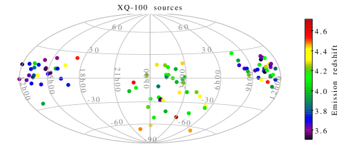
Figure 1: Sky distribution of XQ-100 sources. The color scale indicates emission redshifts.

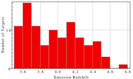
Figure 2: XQ-100 emission redshifts.

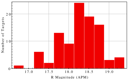
Figure 3: XQ-100 $R$-magnitudes (APM).

2.2 Observations

The observations were carried out in “service mode” between April 1, 2012, and March 26, 2014. During this time XSHOOTER was mounted on unit 2 of the VLT. Service mode allows the user to define the Observation Blocks (OBs), which contain the instrument setup and are carried out by the observatory under the required weather conditions.

Table 1 summarizes the requested conditions of XQ-100. The airmass constraint was set according to each target’s declination such that the target was observable above the set constraint for at least 2 hours. The requested constraints on sky brightness were fraction of lunar illumination $<0.5$ and minimum moon distance 45 degrees. The targets were split into two samples, brighter and fainter than magnitude $R_{\rm APM}=18.0$. The seeing constraint was set to $1.0$″ for the bright sample and $0.8$″ for the faint sample. ESO Large Programmes are granted high priority status, which means that observations out of specifications are repeated and eventually carried over to the following semester until the constraints are met (to within $\approx 10$ %). In our case 13 targets were observed more than once because of interrupted OBs or because of ADC issues (§ 2.2.1). As a consequence of this process, 88 XQ-100 targets were observed within specifications, and 12 almost within specifications (i.e., the constraints were worse by $\lesssim 10$ %).

Table 1: Requested observing conditions

Seeing	$1.0$″ (bright), $0.8$″ (faint)
Sky transparency	Clear
	$\delta>+20$: $<1.6$
Airmass	$+10<\delta<20$: $<1.5$
	$0<\delta<+10$: $<1.4$
	$\delta<0$: $<1.3$
% of lunar illumination	50%
Moon distance	45 degrees

Table 2: Instrument setup

Arm	Wavelength range	Slit width	Resolving power	Num. of exposures		Integration time (s)
	[nm]	(″)	$\lambda/\Delta\lambda$	bright	faint	bright	faint
UVB	315–560	1.0	4 350	2	4	890	880
VIS	540–1 020	0.9	7 450	2	4	840	830
NIR	1 000–2 480a	0.9	5 300	2	4	900	900

^a1 000–1 800 nm when the $K$-band filter was used; see § 2.2.

Table 2 summarizes the instrument setup. XSHOOTER has three spectroscopic arms, UVB, VIS and NIR, each with its own set of shutter, slit mask, cross-dispersive element, and detector. In order to obtain signal-to-noise ratios, that are as uniform as possible, XQ-100 integration times varied across the samples and also across the three spectroscopic arms. The bright sample had two integrations, each with $T_{\rm exp}=890$s in UVB, $T_{\rm exp}=840$s in VIS and $T_{\rm exp}=900$s in the NIR. The faint sample had four exposures, each with $T_{\rm exp}=880$s in the UVB, $T_{\rm exp}=830$s in the VIS, and $T_{\rm exp}=900$s in the NIR. These conditions defined two classes of OBs, which – including acquisition – had a total of $39$ and $70$ minutes duration, respectively. In order to optimize the sky-subtraction in the NIR, the exposures were nodded along the slit by $\pm 2.5$″ from the slit center.

The adopted slit widths were 1.0″ in the UVB and 0.9″ in the VIS and NIR, to match the requested seeing and account for its wavelength dependence. These slit widths provide a nominal resolving power of $4\,350$, $7\,450$, and $5\,300$, respectively. The slit position was always set along the parallactic angle, except for five targets for which it was necessary to avoid contamination of a nearby bright object in the slit; these cases are relevant to a problem with the atmospheric dispersion corrector system (see next Section). Target acquisition was done in the $R$ filter. The UVB and VIS were binned by a factor 2 in the dispersion direction.

For emission redshifts $z>4$, the [OIII]$\lambda$5007 emission line lies out of the $K$-band. For $4.0\la z\la 4.5$, [OII]$\lambda$3727 falls in the gap between the $H$- and $K$-bands. Therefore, the 53 XQ-100 sources having $z>4$ were observed using a $K$-band blocking filter that lowers the sky background where scattered light from the $K$-band affects primarily the $J$-band (Vernet et al., 2011). No blocking filter was used for $z<4$ sources (47) in order to include [OIII]$\lambda$5007 in the wavelength range. We note that Mg ii$\lambda\lambda$2796,2803 is always in the wavelength range. See Fig. 7 for an example of a spectrum presenting the above-mentioned emission lines.

For each exposure, the standard calibration plan of the observatory was used to observe a hot star for telluric corrections. This plan foresees the observation of a telluric standard within 2 hours and 0.2 airmasses of each science observation (but see § 4.1).

2.2.1 ADC issues

In March 2012 ESO reported that the atmospheric dispersion correctors (ADCs) of the UVB and VIS arms started to fail occasionally, leading to possible wavelength-dependent slit losses, potentially worse than if no ADCs were used. In August 2012 the ADCs were disabled for the rest of the observations (at the time of writing the causes of these failures are being investigated).

By August 2012, around 30% of the XQ-100 observations had been executed. After checking our spectra carefully, we noticed the ADC problem had possibly affected 12 of the spectra, which showed an unusually large flux mismatch between the arms (see example in top panel of Fig. 4, which is explained below). The reason for such a mismatch was probably that these targets had been observed at a high enough airmass for a malfunctioning ADC to lead to strong chromatic slit losses.

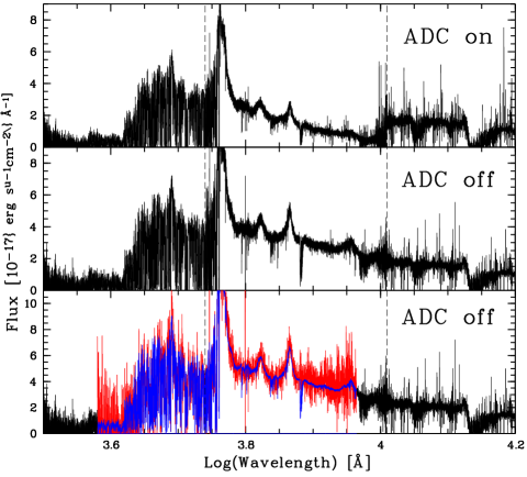
Figure 4: XQ-100 spectra of the same QSO, J1126$-$0124, taken with the faulty ADCs in April 2012 (top panel) and repeated with the disabled ADCs in February 2014 (middle panel). Both observations were executed at a similar airmass of $\approx 1.3$ at the parallactic angle. The dashed lines indicate the boundaries of the XSHOOTER arms. The match is better between the VIS and NIR arms in the middle panel. The bottom panel shows the same February 2014 XQ-100 spectrum but smoothed and rebinned to SDSS resolution (blue line), and rescaled by a factor of 1.3 to match the corresponding SDSS spectrum (overlaid in red). The good match suggests that slit losses in the XQ-100 data are roughly achromatic.

Five out of these 12 OBs were executed a second time with the disabled ADCs and using the parallactic angle. The improvement was evident. The two upper panels of Fig. 4 show XQ-100 spectra of the same OB executed before and after the ADC disabling. We note the effect of the faulty ADCs on the flux levels and slope in the UVB and VIS arms only (top panel), while the NIR arm is not affected, which is expected since this arm does not use an ADC. Conversely, without the ADCs (middle panel) the flux levels have a better match between the arms (spectra were taken at the parallactic angle always). The bottom panel of Fig. 4 shows the XQ-100 spectrum from the middle panel but smoothed and rebinned to SDSS resolution (blue line), and rescaled by a factor of 1.3 to match the corresponding SDSS spectrum (overlaid in red). The good match across wavelengths suggests that slit losses, at least in the SDSS spectral region, are roughly achromatic in the XQ-100 spectra.

Since the accuracy of flux calibrations is unimportant for many of the science applications described in the introduction and an extra exposure might be helpful to increase the S/N, we provide reduced spectra of both observations in these 13 cases and flag them in our database (see Section 5).

The remaining observations in the queue proceeded without the ADCs but making sure that the parallactic angle and the lowest possible airmass was chosen.

3 Data reduction

Extraction of NIR spectra can prove a non-trivial task owing to the high sky-background levels. ESO provides a pipeline to reduce XSHOOTER data, which we have tested. However, in doing so, we noticed that the reduced spectra show systematically large and frequent sky-subtraction residuals in the NIR. Consequently, we opted to implement our own custom pipeline and to reduce XQ-100 data using scripts written in idl by one of us (GDB). Figure 5 shows an example that highlights the differences between the two pipelines in the NIR. Overall, despite some unavoidable residuals, the idl pipeline seems to be more effective than the ESO version available by mid-2014. In the following two sections we describe our pipeline and then provide a qualitative comparison with the ESO version.

Figure 5: Portion of the NIR spectrum of QSO J0003-2603 at $z=4.125$ reduced using the XSHOOTER/Reflex pipeline, version 2.5.2 (top) and our own idl pipeline (bottom). The tickmarks in between spectra indicate Mg ii and Mg i absorption lines in a DLA at $z=3.390$. The bottom spectrum is much less affected by the residuals.

3.1 Custom pipeline

The overall reduction strategy is based on the techniques of Kelson (2003), where operations are performed on the un-rectified 2D frames. To achieve this, we generated 2D arrays of slit position and wavelength that served as the coordinate grid for sky modeling and 1D spectrum extraction. A fiducial set of coordinate arrays for each arm was registered to individual science frames using the measured positions of sky and/or arc lines.

Individual frames were bias subtracted (or dark subtracted in the case of the NIR arm) and flat-fielded. The sky emission in each order was then modeled using a b-spline and subtracted. To avoid adding significant extra noise in the NIR arm, composite dark frames were generated from multiple (typically $\sim 10$) dark exposures with matching integration times. This approach was found to remove the fixed pattern noise in the NIR to the extent that the sky emission could generally be well modeled in each exposure independently, without subtracting a nodded frame, thus avoiding a factor $\sqrt{2}$ penalty in the background noise. The exception to this was the reddest order (2 270-2 480 nm), which is problematic because it is vignetted by a baffle designed to mask stray light (see footnote 2 in § 1) This order was therefore nod-subtracted, and the residual sky emission modeled using a b-spline.

Following sky subtraction, the counts in the 2D frames were flux calibrated using response curves generated from observations of spectro-photometric standard stars. Standards observed close in time to the science observations were generally used. For a limited number of objects, however, the temporally closest star was not optimal and unexpected features were observed in the flux-calibrated spectra. In these cases, a fiducial response curve was used to produce an additional flux-calibrated spectrum.

A single 1D spectrum was then extracted simultaneously from across all orders and all exposures of a given object (in a single arm). Extraction was performed on the non-rectified frames to avoid multiple rebinnings and to keep the error correlation across adjacent pixels to a minimum. The number of exposures for each object ranges between 2 and 12, depending on the number of scheduled exposures (two to four) and on the number of times a given OB was executed (typically one, but two or three in cases of interrupted execution and ADC issues). When observations were spread across several nights, a separate 1D spectrum was extracted for each night.

The one-dimensional spectra were binned using a fixed velocity step. This is the only rebinning involved in the reduction procedure. Wavelength bins for the three arms (UVB: $20$ km s^-1; VIS: $11$ km s^-1; NIR: $19$ km s^-1) were chosen to provide roughly 3 pixels per FWHM, taking the nominal XSHOOTER resolving power for the adopted slits (Table 2). The whole (gap-less) wavelength range is 315 to $1\,800$ nm for spectra taken with the $K$-band blocking filter, and $315$ to $2\,480$ nm for other spectra. Wavelengths were corrected to the vacuum-heliocentric system. When multiple exposures of a single object existed, they were co-added (with the exception of exposures taken with the faulty ADC, which were not included in the co-added spectrum). The stacking was done arm by arm; no attempt was made to merge the arms at this stage, although we do provide joint spectra in the public release (§ 5). In the following, we call these reduced data “raw” to distinguish them from the post-processed data (described in Sections 4 and 5).

Figure 6 shows the distribution of S/N (per pixel) at three different rest-frame wavelengths: $1\,700$ Å (representative of the VIS spectra), $3\,000$ Å (NIR spectra of high-$z$ sources), and $3\,600$ Å (NIR spectra of low-$z$ sources). The respective median signal-to-noise ratios are $33$, $25$ and $43$, as measured in a $\pm 10$ Å window at those rest-frame wavelengths. These values are consistent with the predictions of the XSHOOTER Exposure Time Calculator, which motivated the setup adopted for the OBs.

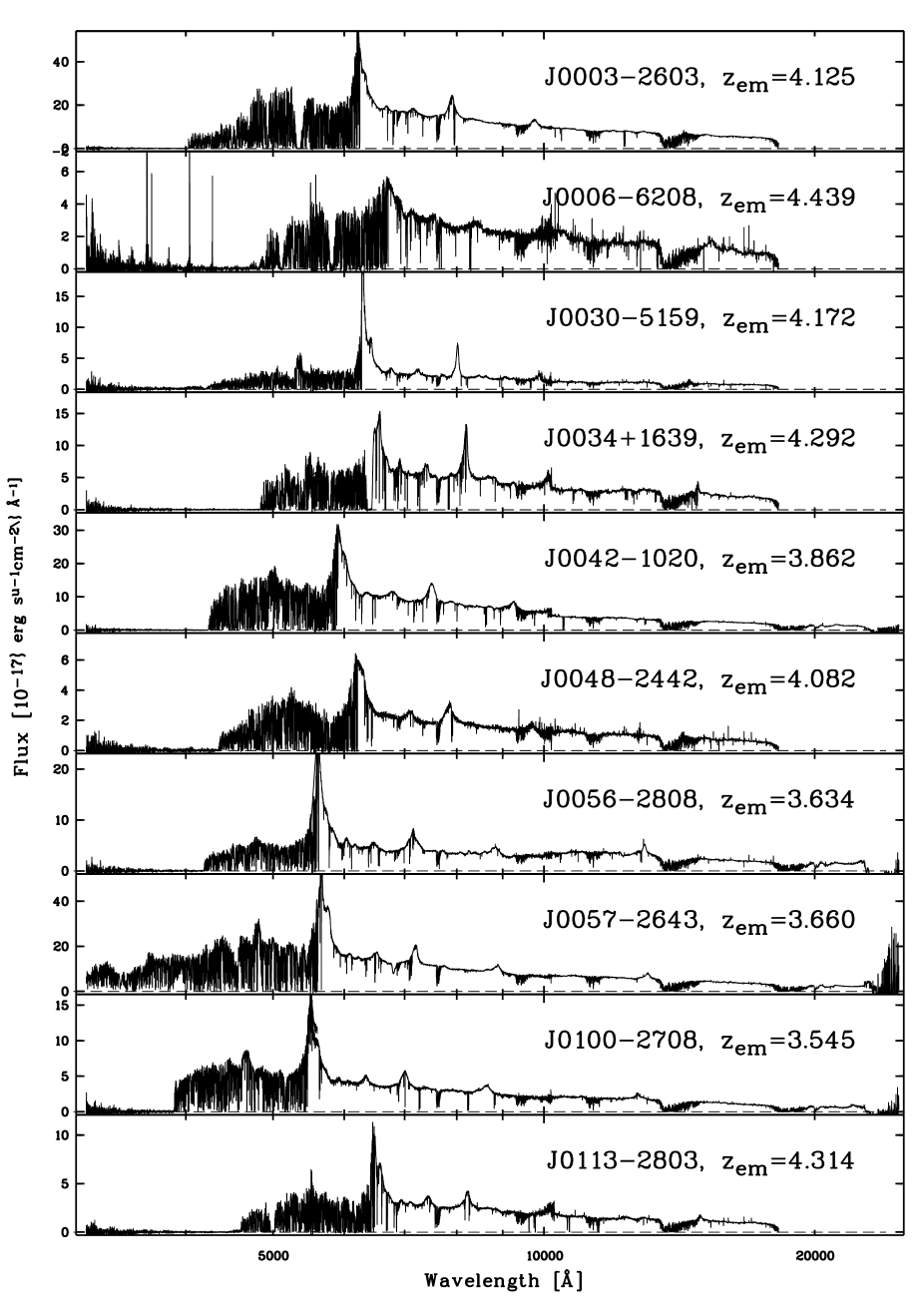
Figure 9: XQ-100 spectra. Names follow the XQ-100 convention (§ 5); see Table LABEL:table_targets for a correspondence with literature names. Emission redshifts were estimated using the result of a principal component analysis (Pâris et al., 2012). The flux has been smoothed with a five-pixel median filter for displaying purposes.

Figures 9 to 18 in Appendix B show all reduced spectra and Fig. 7 shows an example with an expanded wavelength scale.

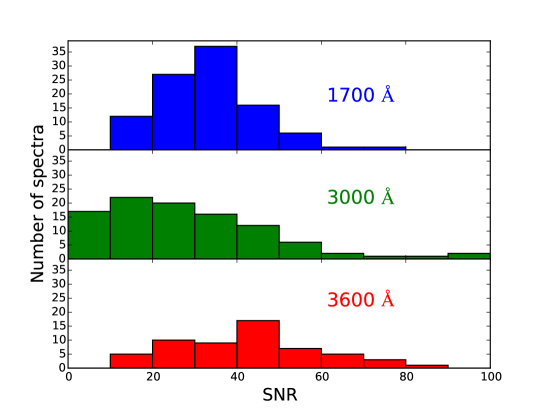
Figure 6: Distribution of pixel signal-to-noise ratios of the co-added spectra at three different rest-frame wavelengths: $1\,700$, $3\,000$, and $3\,600$ Å. The S/N is computed in a window centered at those wavelengths and spanning $\pm 10$ Å. . The $3\,600$ Å histogram has fewer elements because not all spectra cover that wavelength (see § 2.2).

3.2 Accuracy of the flux calibration

Comparison with SDSS spectra (expected to have little aperture loss given the $3\arcsec$ fibers of the spectrograph) shows a systematic underestimation of the flux on the XSHOOTER part ($\left\langle\frac{F_{\mathrm{XSH}}}{F_{\mathrm{SDSS}}}\right\rangle\sim 0.77$), mainly due to slit losses induced by the narrow slits used. As shown in the bottom panel of Fig. 4, these slit losses appear to be roughly achromatic.

In some cases the flux values in adjacent arms (especially VIS and NIR) do not match exactly and a gap is observed. In general we expect a mild mismatch which probably depends on seeing, since slit widths are different in each arm and the standard stars, used for flux calibration, are all taken with a 5″ slit. However, in six spectra a large mismatch is observed ($\approx 30$% across arms), which cannot be attributed to slit losses only. These spectra are: J0113-2803, J1013$+$40650, J1524$+$2123, J1552$+$1005, J1621$-$0042, and J1723$+$2243. For these particular cases, three possible causes were identified: (1) the ADC issue (§ 2.2.1); (2) a sudden interruption in the OB execution, which produced UVB and VIS frames with shorter integration time (when this happens, NIR frames are automatically discarded); or (3) problems with flat-fielding. Since an ad hoc treatment of individual targets was beyond the scope of this release and would have compromised the consistency of the reduction process, we decided not to undertake any further action in this direction.

Thus, flux calibration of XQ-100 spectra should not be taken as absolute. The spectral shape is correctly reconstructed and the flux values can be taken as order-of-magnitude estimates, but users of the public data release may want to refer to photometry when an accurate flux measurement is needed.

Figure 7: XQ-100 spectrum of QSO J1117+1311 at $z=3.622$, a representative case of the whole sample in terms of S/N. The flux is not corrected for telluric absorption (§ 4.1) or rebinned for display purposes. Some emission lines are marked. The red line depicts a manually placed continuum made of cubic splines (see § 4.2 for details). The complete set of XQ-100 spectra is shown in Figs. 9 to 18.

3.3 Comparison with ESO pipeline

The ESO pipeline is run through an environment called Reflex (Freudling et al., 2013), which allows the user to organize the scientific and calibration files and to execute the pipeline in an interactive and graphical fashion. A qualitative comparison between version 2.5.2 of the ESO pipeline and our custom pipeline is as follows:

• Wavelength calibration: The ESO pipeline performs a two-step wavelength calibration of raw spectra, using arc lamp frames. In the first step, the positions of the order edges and arc lines are predicted from a physical model of the instrument. In the second step, a 2D mapping from the detector space to the $(\lambda,s)$ space is computed, where $s$ is the position of the pixel along the slit. This mapping is used to produce the final 2D rectified spectrum. Conversely, our custom-built idl package starts with 2D $\lambda$ and $s$ coordinate frames that have been carefully calibrated for a single reference exposure, and then shifts these frames to match other exposures using the measured positions of sky (VIS, NIR) or arc (UVB) lines. As a consequence, the cascade for the idl package is simpler and the overall execution time (data retrieval+processing) is generally shorter.

• Sky subtraction: Both tools implement the Kelson (2003) algorithm for optimal sky subtraction. For reasons that remain unclear, the idl package provides much better results than the ESO pipeline. Residuals of sky-line subtraction in the NIR arm are consistently higher in spectra obtained with the ESO pipeline, as seen in Fig. 5.

• Object tracing: In the ESO pipeline, the position of the object is extracted from the 2D rectified (i.e. rebinned) spectrum; in MANUAL mode, the position of the centroid and the trace width are both set constant. The idl package fits the object trace directly on the detector space; when the trace is too faint, it is interpolated from the adjacent orders based on offsets from a standard star trace. Optimal extraction is performed using a variant of the Horne (1986) algorithm.

• Coaddition of spectra: The ESO pipeline coadds multiple “nodding” exposures by aligning the object trace in the 2D rectified spectra. Coaddition of already rebinned spectra is not recommended, as it introduces a correlation between the error in adjacent pixels. Conversely, the idl package does not attempt to add the 2D frames. Instead, it optimally extracts a single 1D spectrum from all exposures in the same arm for a given object.

• Ease of use: The ESO pipeline can be run automatically through the Reflex interface. The same is true for the idl package, which is easily scriptable. One advantage of the latter is the possibility of obtaining both individual and co-added spectra from an arbitrarily large set of exposures in a single run, shortening the overall execution time.

4 Post-processing

In addition to the (approximately) flux calibrated spectra, we deliver to the community two other higher level science data products: telluric-corrected spectra and QSO continuum fits.

4.1 Removal of telluric features

Telluric absorption affects spectra in both the VIS and NIR arms. Correcting these airmass-dependent spectral features using standard star spectra, even taken relatively close in time to the science targets, can become highly non-trivial owing to the rapidly changing NIR atmospheric transparency. Instead, we opted to derive corrections using model transmission spectra based on the ESO SKYCALC Cerro Paranal Advanced Sky Model (Noll et al., 2012; Jones et al., 2013), version 1.3.5. The SKYCALC models are a function of both airmass and precipitable water vapor (PWV) and span a grid in these parameters providing a spectral resolution of $R=100\,000$. These corrections were applied to individual-epoch spectra of all XQ-100 sources. Fig. 8 shows an example of the results.

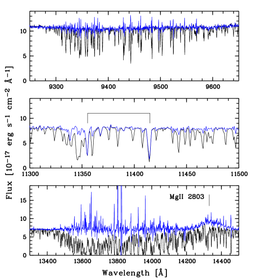
Figure 8: Spectrum of QSO J0003$-$2603 at $z=4.125$ before (black) and after (blue) telluric corrections. Three spectral windows with strong telluric absorption are shown. In the middle panel the tickmarks above the spectrum indicate two Fe ii absorption lines, $\lambda 2586$ and $\lambda 2600$ Å, associated with the $z=3.390$ DLA. In the bottom panel we note how the Mg ii emission line stands out in the corrected spectrum.

Synthetic atmospheric transmission spectra based on the SKYCALC models were fit separately to each VIS and NIR 1D spectrum as a way to remove the observed telluric absorption features. The sky model airmass and PWV parameters, as well as a velocity offset and Gaussian FWHM smoothing kernel, were interactively adjusted for each spectrum in order to minimize the residuals in the model-subtracted spectrum over spectral regions observed to have moderate amounts of absorption, e.g., $\sim$7150$-$7350Å, $\sim$7620$-$7680Å, $\sim$8120$-$8350Å, $\sim$8950$-$9250Å, $\sim$9400$-$9600Å, $\sim$11000$-$11600Å, and $\sim$14600$-$15000Å. Following this initial, interactive parameter selection, an automated parameter selection was performed that searched a grid of only airmass and PWV values in a narrow grid, relative to the best-selected parameters from the interactive search. Multiple sets of best-fit automated parameters were determined for each spectrum by maximizing the S/N measured in the model-subtracted VIS or NIR spectrum over each of the wavelength regions listed above, separately, as well as an average S/N based on all VIS or NIR regions, respectively. The set of parameters used to create the final, telluric-correction model was selected by eye from these multiple, best, model-subtracted spectra.

Owing to the complex nature of correcting for the telluric absorption in this way, which is affected by, for example, the degeneracy between fit parameters and the variable atmospheric conditions during each observation, a single set of parameters generally was not able to optimize the telluric absorption correction at all wavelengths. Similarly, a single quantitative measure of “best” was not attempted. So while the final correction remains somewhat subjective, this allowed an optimization of the correction over the wavelength regions of greatest interest, e.g., near QSO emission lines, such as C iv or Mg ii (see bottom panel of Fig. 8) that will be important for further analysis, and varies for objects at different redshifts.

The telluric correction models were fit to all available 1D spectra. This includes individual-epoch spectra for all objects, as well as spectra co-added from multiple epochs. We note, however, that these model-subtracted, co-added spectra are of poorer quality than those from the individual epochs. This is a result of the coadd of the multiple epochs being done to the pre-telluric-corrected, 2D, unrectified images, which was done to avoid rebinning multiple times. However, this necessarily results in mixed atmospheric features in the co-added spectrum. Such features cannot be cleanly fit by the atmospheric models. In these cases, an argument can be made for coadding the telluric-corrected, 1D spectra instead of the uncorrected 2D frames, even if an additional rebinning is required; however, such post-processing decisions and procedures are left to the user.

4.2 Continuum fitting

For each arm the manually placed continuum was determined by selecting points along the QSO continuum free of absorption (by eye) as knots for a cubic spline. The code used for the continuum fitting is available at https://github.com/trystynb/ContFit.

For all sightlines, the continuum placement was visually inspected and adjusted such that the final fit resides within the variations of regions with clean continuum. The accuracy of the fits is as good as or better than the S/N of these clean continuum regions. As the continuum fits were created for accurate DLA metal line abundances (Berg et al., 2016), the fits around DLA metal lines have undergone multiple revisions compared to other regions of the spectra. The continuum placement in the Ly$\alpha$ forest is highly subjective due to the lack of clean QSO continuum (e.g. Kirkman et al., 2005), and is particularly difficult to identify around the Ly$\alpha$ absorption of DLAs. The continuum around a DLA Ly$\alpha$ absorption feature in the XQ-100 sightlines requires further refinement on a case-by-case basis to match the N(Hi) fits of the Ly$\alpha$ wings, as implemented in Sánchez-Ramírez et al. (2016).

In regions where the QSO continuum is absorbed, the spline knots were placed at a constant (high) flux at: (i) The Lyman limit if one or more obvious Lyman limits systems are clearly present, and (ii) telluric features (near observed wavelengths 6900Å, 7600Å, 9450Å, 11400Å, and 14000Å). In some sightlines, there are strong absorption features on top of the Ly$\alpha$ emission line of the QSO, such that the continuum of the emission line is not well constrained (particularly near the peak of the emission). In cases with this strong absorption present, the continuum on the Ly$\alpha$ emission is assumed to follow the interpolation from the cubic spline fit to the surrounding continuum knots.

An example of the continuum presented above is shown in Fig. 7. We note, however, that we provide continua separately for each arm-by-arm spectrum, not for the joint spectra.

5 Description of science data products

All the XQ-100 raw data, along with calibration files are available through the ESO archive (http://archive.eso.org/eso/eso_archive_main.html). Advanced science data products (SDP) are publicly available in the form of ESO Phase 3 material (http://archive.eso.org/wdb/wdb/adp/phase3_main/form).

The full XQ-100 target list is provided in Table LABEL:table_targets. We also provide a summary file with basic properties (e.g., coordinates and redshifts), spectroscopic properties (e.g., S/N at different rest frame wavelengths), multi-wavelength photometric information, and other spectroscopic data available for each XQ-100 QSO. The detailed content of this summary file is given in Table LABEL:table_parameters. We format all the data file names in the same fashion (JNNNNsNNNN) and we provide this standardized name.

Two types of data are provided for each target: (1) individual UVB, VIS, and NIR spectra, also with telluric correction and fitted QSO continuum; and (2) a joint spectrum of the three arms together.

5.1 Individual UVB, VIS, and NIR spectra

There are four different main data files per QSO in the XQ-100 sample: one with the reduced 1D spectrum in the UVB arm, one for the VIS arm, one for the NIR reduced in “stare” mode, and one with the 1D NIR spectrum reduced in nodding mode when available, i.e., when $z<4$ (targets observed without the K-band blocking filter).

Each spectrum file contains wavelength, flux, error on the flux, sky-subtracted flux, and associated error (§ 4.1).

When a target was observed more than once (because the observing specifications were not met the first time; see § 2.2), we produced individual spectra of each execution of the OB. Whenever possible, we also produced a co-added spectrum putting together all executions. In the co-added spectra we discarded the first exposures either when they were affected by the ADC issue, or when they were interrupted (as their contribution was negligible due to the short integration time). We define as “primary” spectra those with the best achievable S/N. For targets observed more than once, these correspond to the co-added spectra.

A breakdown of the different spectra provided is shown in Table 5.

5.2 Joint spectra

Joint spectra contain the three arms merged into a single spectrum. Fluxes from the VIS and NIR arms were rescaled to match the UVB flux level. We first computed the VIS scaling factor (using the UVB-VIS superposition); then, after correcting the VIS, we computed the NIR scaling factor (using the VIS-NIR superposition). In both cases, the scaling factor was defined as the ratio of the two median fluxes in the superposition region. After rescaling, the limit wavelength between UVB and VIS arms was set at 5 600 Å and at 10 125 Å between the VIS and NIR arms. The three arms were finally pieced together to create a single spectrum. For targets observed without the K-band blocking filter, the last order of the NIR was taken from the products of the nodding reduction, which are similarly rescaled, cut at 22 700 Å, and pieced together. The resulting spectrum was finally cut in the blue end at 3 000 Å and in the red end at 25 000 Å (for targets observed without the K-band blocking filter) and at 18 000 Å (for other targets), to guarantee a comparable wavelength span across the data set. We note that the procedure described above is the result of several choices that may not be appropriate for all scientific analyses.

5.3 Data format

All the spectra we release are binary FITS files. The naming convention is

• for the individual arm-by-arm spectra: target_arm_exec.fits

• for the joint spectra: target.fits

where target is the target name in shortened J2000 coordinates (JNNNN+NNNN or JNNNN$-$NNNN), arm is the spectral arm, including the optional nodding suffix for the NIR (uvb, vis, nir, or nir_nod), and exec is the optional execution suffix (_1, _2, _3, or blank). The individual arm-by-arm spectrum without the exec suffix is to be regarded as the primary spectrum for the given target in all cases. The list of table columns is

• for the individual arm-by-arm spectra: WAVE, FLUX, ERR_FLUX, CONTINUUM, FLUX_TELL_CORR, ERR_FLUX_TELL_CORR

• for the joint spectra: WAVE, FLUX, ERR_FLUX

The column description is as follows:

• WAVE: wavelength in the vacuum-heliocentric system (Å);

• FLUX: flux density (erg cm^-2 s^-1 Å^-1);

• ERR_FLUX: error of the flux density (erg cm^-2 s^-1 Å^-1);

• CONTINUUM: fitted continuum (erg cm^-2 s^-1 Å^-1);

• FLUX_TELL_CORR: same as flux, but with the telluric features removed (erg cm^-2 s^-1 Å^-1);

• ERR_FLUX_TELL_CORR: error of flux_tc (erg cm^-2 s^-1 Å^-1)

6 Summary

We have presented XQ-100, a legacy survey of $100$ $z_{\rm em}\simeq 3.5$–$4.5$ QSOs observed with VLT/XSHOOTER. We have provided a basic description of the sample, along with details of the observations, and details of the data reduction process. We have also described the format and organization of the publicly available data, which include spectra corrected for atmospheric absorption and a continuum fit.

XQ-100 provides the first large uniform sample of high-redshift QSOs at intermediate-resolution and with simultaneous rest-frame UV/optical coverage. In terms of number of QSOs this volume represents a $30\%$ increase over the whole extant XSHOOTER sample. The released spectra are of superb quality, having median S/N $\sim 30$, $25$, and $40$ at resolutions of $\sim 30$–$50$ km s^-1, depending on wavelength. We have indicated that these properties enable a wide range of high-redshift research and soon look forward to seeing the results of this three-year effort in the form of new discoveries and contributions to the field.

Appendix A Tables

Table 3: Summary of XQ-100 target properties

XQ-100 name	NED Name	RA	DEC	Redshift	$R_{\rm APM}$	SNR1700	SNR3000	SNR3600
(1)	(2)	(3)	(4)	(5)	(6)	(7)	(8)	(9)
J0003–2603	HB89 0000–263	00 03 22.79	–26 03 19.4	4.125	17.37	79	99	-1
J0006–6208	BR J0006–6208	00 06 51.60	–62 08 0.78	4.440	19.25	20	22	-1
J0030–5159	BR J0030–5159	00 30 34.47	–51 29 43.6	4.173	18.57	18	22	-1
J0034+1639	PSS J0034+1639	00 34 54.71	+16 39 18.2	4.292	18.03	28	30	-1
J0042–1020	SDSS J004219.74–102009.4	00 42 19.73	–10 20 12.2	3.863	18.23	52	48	58
J0048–2442	BRI J0048–2442	00 48 34.37	–24 42 06.9	4.083	19.22	20	18	-1
J0056–2808	HB89 0053–284	00 56 24.87	–28 08 33.3	3.635	18.10	29	22	43
J0057–2643	HB89 0055–269	00 57 58.14	–26 43 12.9	3.661	17.72	46	20	62
J0100–2708	PMN J0100–2708	01 00 12.47	–27 08 52.1	3.546	18.87	30	6	30
J0113–2803	BRI J0113–2803	01 13 44.17	–28 03 17.9	4.314	18.67	30	37	-1
J0117+1552	PSS J0117+1552	01 17 31.05	+15 52 14.2	4.243	17.22	40	62	-1
J0121+0347	PSS J0121+0347	01 21 26.21	+03 47 04.7	4.125	18.33	31	30	-1
J0124+0044	SDSS J0124+0044	01 24 03.97	+00 44 31.4	3.837	17.75	34	41	48
J0132+1341	PSS J0132+1341	01 32 09.98	+13 41 35.9	4.152	18.53	32	30	-1
J0134+0400	PSS J0134+0400	01 33 40.47	+04 00 58.5	4.185	18.32	48	52	-1
J0137–4224	BRI J0137–4224	01 37 24.36	–42 24 14.9	3.971	18.77	17	18	17
J0153–0011	SDSS J015339.60–001104.8	01 53 39.73	–00 11 06.1	4.195	18.87	15	18	-1
J0211+1107	PSS J0211+1107	02 11 20.10	+11 07 14.5	3.973	18.20	22	26	25
J0214–0518	PMN J0214–0518	02 14 29.41	–05 17 45.4	3.977	18.42	31	28	24
J0234–1806	BR J0234–1806	02 34 55.03	–18 06 11.3	4.305	18.79	28	30	-1
J0244–0134	BRI 0241–0146	02 44 01.83	–01 34 06.3	4.055	18.18	39	44	-1
J0247–0555	BR 0245–0608	02 47 56.70	–05 56 00.0	4.234	18.65	22	29	-1
J0248+1802	PSS J0248+1802	02 48 54.37	+18 02 47.0	4.439	17.71	26	40	-1
J0255+0048	SDSS J025518.57+004847.4	02 55 18.70	+00 48 46.5	4.003	18.31	30	32	22
J0307–4945	BR J0307–4945	03 07 22.57	–49 45 45.6	4.716	18.76	37	82	-1
J0311–1722	BR J0311–1722	03 11 15.38	–17 22 48.4	4.034	17.73	39	37	-1
J0401–1711	BR J0401–1711	04 03 56.82	–17 03 22.0	4.227	18.69	21	28	-1
J0415–4357	BR J0415–4357	04 15 15.18	–43 57 50.7	4.073	18.81	16	28	-1
J0424–2209	BR J0424–2209	04 26 10.47	–22 02 17.5	4.329	-1	26	33	-1
J0523–3345	BR J0523–3345	05 25 05.95	–33 43 4.44	4.385	18.37	39	65	-1
J0529–3526	BR J0529–3526	05 29 15.98	–35 26 01.2	4.418	18.94	22	25	-1
J0529–3552	BR J0529–3552	05 29 20.94	–35 52 31.8	4.172	18.29	13	14	-1
J0714–6455	BR J0714–6455	07 14 30.92	–64 55 10.3	4.465	18.35	29	48	-1
J0747+2739	SDSS J074711.15+273903.3	07 47 11.17	+27 39 00.8	4.133	17.24	27	34	-1
J0755+1345	SDSS J075552.41+134551.1	07 55 52.43	+13 45 49.6	3.663	18.75	29	9	32
J0800+1920	SDSS J080050.27+192058.9	08 00 50.26	+19 20 56.3	3.948	18.27	29	28	33
J0818+0958	SDSS J081855.78+095848.0	08 18 55.75	+09 58 44.9	3.656	17.69	38	1	44
J0833+0959	SDSS J083322.50+095941.2	08 33 22.50	+09 59 38.6	3.716	18.52	33	13	37
J0835+0650	SDSS J083510.92+065052.8	08 35 10.91	+06 50 51.0	4.007	17.95	33	34	20
J0839+0318	SDSS J083941.45+031817.0	08 39 41.58	+03 18 18.2	4.230	17.85	12	19	-1
J0920+0725	SDSS J092041.76+072544.0	09 20 41.72	+07 25 41.2	3.646	18.53	40	3	37
J0935+0022	SDSS J093556.91+002255.6	09 35 56.87	+00 22 52.8	3.747	17.78	27	15	25
J0937+0828	SDSS J093714.48+082858.6	09 37 14.51	+08 28 56.2	3.704	18.15	23	4	37
J0955–0130	BRI 0952–0115	09 55 00.01	–01 30 08.4	4.418	18.66	35	37	-1
J0959+1312	SDSS J095937.11+131215.4	09 59 37.23	+13 12 17.6	4.092	16.87	54	76	-1
J1013+0650	J101347+065015	10 13 47.48	+06 50 16.6	3.809	18.38	30	22	38
J1018+0548	J101818+054822	10 18 18.57	+05 48 20.7	3.515	18.14	30	14	38
J1020+0922	J102040+092254	10 20 40.74	+09 22 53.1	3.640	18.02	22	4	19
J1024+1819	SDSSJ1024+1819	10 24 56.78	+18 19 07.1	3.524	17.89	26	2	27
J1032+0927	J103221+092748	10 32 21.26	+09 27 47.5	3.985	17.94	27	22	17
J1034+1102	J103446+110214	10 34 46.55	+11 02 12.0	4.269	18.18	33	35	-1
J1036–0343	BR 1033–0327	10 36 23.63	–03 43 21.0	4.531	19.18	19	47	-1
J1037+2135	SDSSJ1037+2135	10 37 30.43	+21 35 29.8	3.626	17.69	52	11	62
J1037+0704	J103732+070426	10 37 32.31	+07 04 23.7	4.127	18.33	49	46	-1
J1042+1957	SDSSJ1042+1957	10 42 34.02	+19 57 16.3	3.630	18.11	36	12	37
J1053+0103	SDSS J105340.75+010335.6	10 53 40.82	+01 03 33.5	3.663	19.11	36	8	37
J1054+0215	J105434+021551	10 54 34.33	+02 15 51.3	3.971	18.03	14	13	12
J1057+1910	J105705+191042	10 57 05.53	+19 10 43.7	4.128	17.87	19	21	-1
J1058+1245	J105858+124554	10 58 58.51	+12 45 53.8	4.341	17.64	26	35	-1
J1103+1004	J110352+100403	11 03 52.72	+10 04 0.48	3.607	18.61	44	14	64
J1108+1209	J110855+120953	11 08 55.56	+12 09 51.7	3.679	18.40	40	10	62
J1110+0244	J111008+024458	11 10 08.81	+02 44 57.3	4.146	17.59	30	36	-1
J1111–0804	BRI 1108–0747	11 11 13.89	–08 04 03.9	3.922	18.82	43	38	55
J1117+1311	J111701+131115	11 17 01.97	+13 11 13.0	3.622	18.28	39	9	47
J1126–0126	J112617–012632	11 26 17.54	–01 26 34.2	3.635	18.70	22	4	24
J1126–0124	J112634–012436	11 26 34.42	–01 24 38.0	3.765	18.53	27	15	21
J1135+0842	J113536+084218	11 35 36.55	+08 42 17.3	3.834	18.26	55	49	53
J1201+1206	HB89 1159+123	12 01 48.05	+12 06 28.2	3.522	17.32	52	4	83
J1202–0054	SDSSJ1202–0054	12 02 10.06	–00 54 27.9	3.592	18.49	23	3	23
J1248+1304	J124837+130440	12 48 37.39	+13 04 39.2	3.721	18.14	39	22	53
J1249–0159	J124957–015928	12 49 57.40	–01 59 29.8	3.629	17.47	37	18	46
J1304+0239	J130452+023924	13 04 52.60	+02 39 21.8	3.648	18.55	47	13	54
J1312+0841	J131242+084105	13 12 42.94	+08 41 02.8	3.731	18.41	33	30	46
J1320–0523	J1320299–052335	13 20 30.12	–05 23 36.3	3.717	17.81	41	18	65
J1323+1405	J132346+140517	13 23 46.21	+14 05 16.4	4.054	18.60	23	21	-1
J1330–2522	BR J1330–2522	13 30 52.17	–25 22 18.1	3.949	18.46	39	45	44
J1331+1015	SDSS J133150.69+101529.4	13 31 50.77	+10 15 27.5	3.852	18.76	33	33	40
J1332+0052	J133254+005250	13 32 54.60	+00 52 48.3	3.508	18.43	41	17	57
J1336+0243	J133653+024338	13 36 53.43	+02 43 35.5	3.801	18.62	33	20	36
J1352+1303	J135247+130311	13 52 48.09	+13 03 09.8	3.706	18.35	14	3	15
J1401+0244	J1401+0244	14 01 46.52	+02 44 37.7	4.408	18.41	39	47	-1
J1416+1811	SDSSJ1416+1811	14 16 08.32	+18 11 46.1	3.593	18.19	24	6	23
J1421–0643	PKS B1418–064	14 21 07.93	–06 43 57.6	3.688	19.03	40	17	45
J1442+0920	J144250+092001	14 42 50.12	+09 19 58.9	3.532	17.21	42	7	46
J1445+0958	SDSSJ1445+0958	14 45 16.62	+09 58 34.9	3.562	17.64	40	4	43
J1503+0419	J150328+041949	15 03 29.01	+04 19 47.3	3.692	18.01	41	18	45
J1517+0511	SDSSJ1517+0511	15 17 56.20	+05 11 00.7	3.555	18.31	41	5	38
J1524+2123	SDSSJ1524+2123	15 24 36.17	+21 23 07.0	3.600	17.25	27	8	42
J1542+0955	J154237+095558	15 42 37.62	+09 56 01.2	3.986	18.18	31	24	16
J1552+1005	J155255+100538	15 52 55.22	+10 05 37.0	3.722	18.63	35	11	49
J1621–0042	J1621–0042	16 21 17.04	–00 42 52.9	3.711	17.67	34	27	77
J1633+1411	J163319+141142	16 33 19.69	+14 11 39.7	4.365	18.72	31	45	-1
J1658–0739	J1658–0739	16 58 44.20	–07 39 16.4	3.750	-1	37	45	78
J1723+2243	PSS J1723+2243	17 23 23.13	+22 43 54.7	4.531	18.71	16	99	-1
J2215–1611	BR 2212–1626	22 15 27.26	–16 11 34.3	3.995	-1	40	54	45
J2216–6714	BR 2213–6729	22 16 51.98	–67 14 41.2	4.479	18.57	21	40	-1
J2239–0552	J2239536–055219	22 39 53.62	–05 52 21.3	4.557	18.30	10	26	-1
J2251–1227	BR 2248–1242	22 51 18.19	–12 27 05.1	4.157	18.55	34	58	-1
J2344+0342	PSS J2344+0342	23 44 03.05	+03 42 24.3	4.248	18.16	32	33	-1
J2349–3712	BR J2349–3712	23 49 13.56	–37 12 59.8	4.219	19.19	21	29	-1

Table 3: continued.

Columns:

(1) Target name used throughout this paper and also given to the files associated with each object; (2) target’s NED name, also found in the SDP headers; (3) right ascension in sexagesimal degrees (J2000); (4) declination in sexagesimal degrees (J2000); (5) QSO redshift estimated using the result of a principal component analysis (Pâris et al., 2012); (6) APM $R$-magnitude. When the magnitude was not found, the value was set to $-1$; (7) , (8) and (9) average pixel SNR in the co-added spectrum near rest-frame wavelengths $1\,700$, $3\,000$ and $3\,600$ Å, respectively; set to $-1$ if wavelength was not covered, i.e., for spectra taken with the K-band blocking filter ($z_{\rm em}>4$ sources).

Table 4: Parameters associated with each XQ-100 object in the public repository

Column	Name	Format	Description
1	OBJECT	STRING	target designation
2	RA_J2000	DOUBLE	target right ascension (deg, J2000.0)
3	DEC_J2000	DOUBLE	target declination (deg, J2000.0)
4	Z_QSO	FLOAT	quasar emission redshift (PCA)
5	N_OBS	SHORT	number of observing epochs
6	MJD_OBS	FLOAT	start of observations (d)
7	MJD_OBS_1	FLOAT	start of observations (1st exec. only) (d)
8	MJD_OBS_2	FLOAT	start of observations (2nd exec. only) (d)
9	MJD_OBS_3	FLOAT	start of observations (3rd exec. only) (d)
10	MJD_END	FLOAT	end of observations (d)
11	MJD_END_1	FLOAT	end of observations (1st exec. only) (d)
12	MJD_END_2	FLOAT	end of observations (2nd exec. only) (d)
13	MJD_END_2	FLOAT	end of observations (3rd exec. only) (d)
14	SEEING_MIN	FLOAT	min. seeing from ESO.TEL.IA.FWHM keyw.
15	SEEING_MIN_1	FLOAT	min. seeing from ESO.TEL.IA.FWHM keyw. (1st exec. only)
16	SEEING_MIN_2	FLOAT	min. seeing from ESO.TEL.IA.FWHM keyw. (2nd exec. only)
17	SEEING_MIN_3	FLOAT	min. seeing from ESO.TEL.IA.FWHM keyw. (3rd exec. only)
18	SEEING_MAX	FLOAT	max. seeing measured at the start or at the end of integrations
19	SEEING_MAX_1	FLOAT	max. seeing from ESO.TEL.IA.FWHM keyw. (1st exec. only)
20	SEEING_MAX_2	FLOAT	max. seeing from ESO.TEL.IA.FWHM keyw. (2nd exec. only)
21	SEEING_MAX_3	FLOAT	max. seeing from ESO.TEL.IA.FWHM keyw. (3rd exec. only)
22	SNR_170	FLOAT	S/N in a $\pm$1 nm window at 170 nm (rest-frame)
23	SNR_170_1	FLOAT	S/N in a $\pm$1 nm window at 170 nm (1st exec. only) (rest-frame)
24	SNR_170_2	FLOAT	S/N in a $\pm$1 nm window at 170 nm (2nd exec. only) (rest-frame)
25	SNR_170_3	FLOAT	S/N in a $\pm$1 nm window at 170 nm (3rd exec. only) (rest-frame)
26	SNR_300	FLOAT	S/N in a $\pm$1 nm window at 300 nm (rest-frame)
27	SNR_300_1	FLOAT	S/N in a $\pm$1 nm window at 300 nm (1st exec. only) (rest-frame)
28	SNR_300_2	FLOAT	S/N in a $\pm$1 nm window at 300 nm (2nd exec. only) (rest-frame)
29	SNR_300_3	FLOAT	S/N in a $\pm$1 nm window at 300 nm (3rd exec. only) (rest-frame)
30	SNR_360	FLOAT	S/N in a $\pm$1 nm window at 360 nm (rest-frame)
31	SNR_360_1	FLOAT	S/N in a $\pm$1 nm window at 360 nm (1st exec. only) (rest-frame)
32	SNR_360_2	FLOAT	S/N in a $\pm$1 nm window at 360 nm (2nd exec. only) (rest-frame)
33	SNR_360_3	FLOAT	S/N in a $\pm$1 nm window at 360 nm (3rd exec. only) (rest-frame)
34	RED_QUAL	SHORT	reduction quality parameter (see above)
35	RED_QUAL_1	SHORT	reduction quality parameter (1st exec. only)
36	RED_QUAL_2	SHORT	reduction quality parameter (2nd exec. only)
37	RED_QUAL_3	SHORT	reduction quality parameter (3rd exec. only)
38	HR_FLAG	SHORT	high-resolution spectrum flag
39	JOHNSON_MAG_B	FLOAT	B magnitudes in Johnson system
40	JOHNSON_MAG_V	FLOAT	V magnitudes in Johnson system
41	JOHNSON_MAG_R	FLOAT	R magnitudes in Johnson system
42	SDSS_PSF_MAG_u	DOUBLE	SDSS PSF u magnitudes
43	SDSS_ERR_PSF_MAG_u	DOUBLE	Error on SDSS PSF u magnitudes
44	SDSS_PSF_MAG_g	DOUBLE	SDSS PSF g magnitudes
45	SDSS_ERR_PSF_MAG_g	DOUBLE	Error on SDSS PSF g magnitudes
46	SDSS_PSF_MAG_r	DOUBLE	SDSS PSF r magnitudes
47	SDSS_ERR_PSF_MAG_r	DOUBLE	Error on SDSS PSF r magnitudes
48	SDSS_PSF_MAG_i	DOUBLE	SDSS PSF i magnitudes
49	SDSS_ERR_PSF_MAG_i	DOUBLE	Error on SDSS PSF i magnitudes
50	SDSS_PSF_MAG_z	DOUBLE	SDSS PSF z magnitudes
51	SDSS_ERR_PSF_MAG_z	DOUBLE	Error on SDSS PSF z magnitudes
52	DR7Q_MATCH	SHORT	match in DR7Q spectroscopy
53	DR7Q_LATE	INT32	DR7Q plate number
54	DR7Q_MJD	INT32	DR7Q spectroscopic MJD (d)
55	DR7Q_FIBER	INT32	DR7Q fiber number (d)
56	DR12Q_MATCH	SHORT	match in DR12Q spectroscopy
57	DR12Q_N	INT32	number of spectroscopic observations in DR12Q
58	DR12Q_PLATE_1	INT32	DR12Q plate number (1st observation)
59	DR12Q_MJD_1	INT32	DR12Q spectroscopic MJD (1st observation) (d)
60	DR12Q_FIBER_1	INT32	DR12Q fiber number (1st observation) (d)
61	DR12Q_PLATE_2	INT32	DR12Q plate number (2nd observation)
62	DR12Q_MJD_2	INT32	DR12Q spectroscopic MJD (2nd observation) (d)
63	DR12Q_FIBER_2	INT32	DR12Q fiber number (2nd observation) (d)
64	FIRST_MATCH	INT32	match in FIRST
65	FIRST_FLUX	DOUBLE	FIRST flux at 20 cm (mJy)
66	FIRST_SNR	DOUBLE	S/N of FIRST detection
67	TMASS_MATCH	SHORT	matched in 2MASS
68	TMASS_MAG_J	DOUBLE	2MASS J magnitudes
69	TMASS_ERR_MAG_J	DOUBLE	error on 2MASS J magnitudes
70	TMASS_SNR_J	DOUBLE	S/N of 2MASS detection in J bands
71	TMASS_MAG_H	DOUBLE	2MASS H magnitudes
72	TMASS_ERR_MAG_H	DOUBLE	error on 2MASS H magnitudes
73	TMASS_SNR_H	DOUBLE	S/N of 2MASS detection in H bands
74	TMASS_MAG_K	DOUBLE	2MASS K magnitudes
75	TMASS_ERR_MAG_K	DOUBLE	error on 2MASS K magnitudes
76	TMASS_SNR_K	DOUBLE	S/N of 2MASS detection in K bands
77	TMASS_RD_FLAG	STRING	2MASS rd flag
78	WISE_MATCH	SHORT	match in WISE
79	WISE_MAG_w1	DOUBLE	WISE w1 magnitudes
80	WISE_ERR_MAG_w1	DOUBLE	error on WISE w1 magnitudes
81	WISE_SNR_w1	DOUBLE	S/N of WISE detection in w1 bands
82	WISE_RCHI2_w1	DOUBLE	WISE reduced chi-squared in w1 bands
83	WISE_MAG_w2	DOUBLE	WISE w2 magnitudes
84	WISE_ERR_MAG_w2	DOUBLE	error on WISE w2 magnitudes
85	WISE_SNR_w2	DOUBLE	S/N of WISE detection in w2 bands
86	WISE_RCHI2_w2	DOUBLE	WISE reduced chi-squared in w2 bands
87	WISE_MAG_w3	DOUBLE	WISE w3 magnitudes
88	WISE_ERR_MAG_w3	DOUBLE	error on WISE w3 magnitudes
89	WISE_SNR_w3	DOUBLE	S/N of WISE detection in w3 bands
90	WISE_RCHI2_w3	DOUBLE	WISE reduced chi-squared in w3 bands
91	WISE_MAG_w4	DOUBLE	WISE w4 magnitudes
92	WISE_ERR_MAG_w4	DOUBLE	error on WISE w4 magnitudes
93	WISE_SNR_w4	DOUBLE	S/N of WISE detection in w4 bands
94	WISE_RCHI2_w4	DOUBLE	WISE reduced chi-squared in w4 bands
95	WISE_CC_FLAG	STRING	WISE confusion and contamination flag
96	WISE_PH_QUAL	STRING	WISE photometric quality flag

Table 4: continued.

Notes on the catalog columns:

1. Object name as designated in the ESO archive.

2-3. The J2000 coordinates (Right Ascension and Declination) in sexagesimal degrees.

4. QSO redshift. The redshift was estimated using the result of a principal component analysis (Pâris et al., 2012).

5. Number of XSHOOTER observations. Most QSOs were observed only once. Thirteen QSOs were observed more than once because of interrupted OBs or ADC issues.

6-9. Modified Julian Day (MJD) at the beginning of XSHOOTER observation. The values for the different executions of the same observing block are also listed separately (when applicable).

10-13. Modified Julian Day (MJD) at the end of XSHOOTER observation. The values for the different executions of the same observing block are also listed separately (when applicable).

14-17. Minimum seeing of XSHOOTER observation, taken from the ESO.TEL.IA.FWHM keyword, expressed in arcsec. The values for the different executions of the same observing block are also listed separately (when applicable).

18-21. Minimum seeing of XSHOOTER observation, taken from the ESO.TEL.IA.FWHM keyword, expressed in arcsec. The values for the different executions of the same observing block are also listed separately (when applicable).

22-25. Average S/N near 1 700 Å (rest frame) computed in the window 1 690-1 710Å. The values for the different executions of the same observing block are also listed separately (when applicable) .

26-29. Average S/N near 3 000 Å (rest frame) computed in the window 2 990-3 010Å. The values for the different executions of the same observing block are also listed separately (when applicable).

30-33. Average S/N near 3 600 Å (rest frame) computed in the window 3 590-3 610Å. The values for the different executions of the same observing block are also listed separately (when applicable).

34-37. Calibration flags for each XSHOOTER observation. The value of the resulting calibration flag is the sum of the five following flags. A value of 0 means no problem to report, 1 means that the VIS spectrum was calibrated using a different standard star, 2 means that there are residual spikes in the UVB spectrum, 4 is set when apparent order-to-order fluctuations in the VIS arm, 8 when the exposure was interrupted, and a value of 16 is set when the exposure was taken with faulty ADCs. The values for the different executions of the same observing block (when applicable) are also listed separately.

38. High-resolution spectroscopy (Keck/HIRES or VLT/UVES) exist for some of the XQ-100 QSOs. The HR_FLAG is set to 1 if a high-resolution spectrum exists, otherwise 0.

39-41.. Magnitudes in the $B$, $V$ and $R$ Johnson filters. These values were retrieved from the CDS (Centre de Données astronomiques de Strasbourg). When the magnitude in one of the filters could not be found, the value was set to $-1$.

42-51. SDSS-DR12 point-spread function magnitudes (Cols.#42, 44, 46, 49, 50) and their associated errors (Cols.#43, 45, 47, 48, 51) in the $u$, $g$, $r$, $i$ and $z$ filters (Alam et al., 2015). Objects outside of the SDSS footprint have associated magnitudes and errors set to $-1$.

52. If a QSO was observed as part of SDSS-I/II (York et al., 2000; Schneider et al., 2010), the DR7Q_MATCHED flag is set to 1, otherwise 0.

53-55. When a SDSS-I/II spectrum is available, the SDSS plate number (Col.#53), spectroscopic MJD (Col.#54) and fiber number (Col.#55).

56. If a QSO was observed as part of SDSS-III (Eisenstein et al., 2011), the DR12Q_MATCHED flag is set to 1, otherwise 0.

57. Number of SDSS-III spectra available.

58-63. When SDSS-III spectra are available, the plate numbers (Cols.#58, 61), spectroscopic MJDs (Cols.#59, 62) and fiber numbers (Col.#60, 63). The values of the first and second observation are listed separately (when applicable).

64. If there is a source in the FIRST radio catalog (version March 2014; Becker, White & Helfand, 1995) within 5″ of the QSO position, the FIRST_MATCHED flag is set to 1, otherwise 0. If the QSO lies outside of the FIRST footprint, it is set to $-1$.

65. FIRST peak flux density at 20 cm, expressed in mJy.

66. S/N of the FIRST source whose flux is given in Col.#65.

67. If there is a source from the Two Micron All Sky Survey All-Sky Data Release Point Source Catalog (2MASS; Cutri et al., 2003) within 5″ of the QSO position, the TMASS_MATCHED is set to 1, otherwise 0.

68-76. $J$, $H$, and $K$ magnitudes (Cols.#68, 71, 74), with their associated error (Cols.#69, 72, 75) and S/N (Cols.#70, 73, 76). We note that 2MASS magnitudes are Vega-based.

77. 2MASS rd_flag gives the meaning of the peculiar values of the magnitudes and errors.

78. If a source from the Wide-field Infrared Survey Explorer AllWISE Data Release Point Source Catalog (WISE; Wright et al., 2010) lies within 5″ of a XQ-100 QSO, the WISE_MATCHED is set to 1, otherwise 0.

79-94. WISE $w1$, $w2$, $w3$, and $w4$ magnitudes (Cols#79, 83, 87, 91), with their associated errors (Cols#80, 84, 88, 92), S/N (Cols#81, 85, 89, 93) and $\chi^{2}$ (Cols#82, 86, 90, 94).

95. WISE contamination and confusion flag.

96. WISE photometric quality flag.

Table 5: Number of reduced spectra

	UVB	VIS	NIR	NIR (nodded)	Merged	Total
Primary	100	100	100	47	100
First execution	8	8	8	5	–
Second execution	8	8	8	5	–
Third execution	2	2	2	1	–
Total	118	118	118	58	100	512

Appendix B Spectra

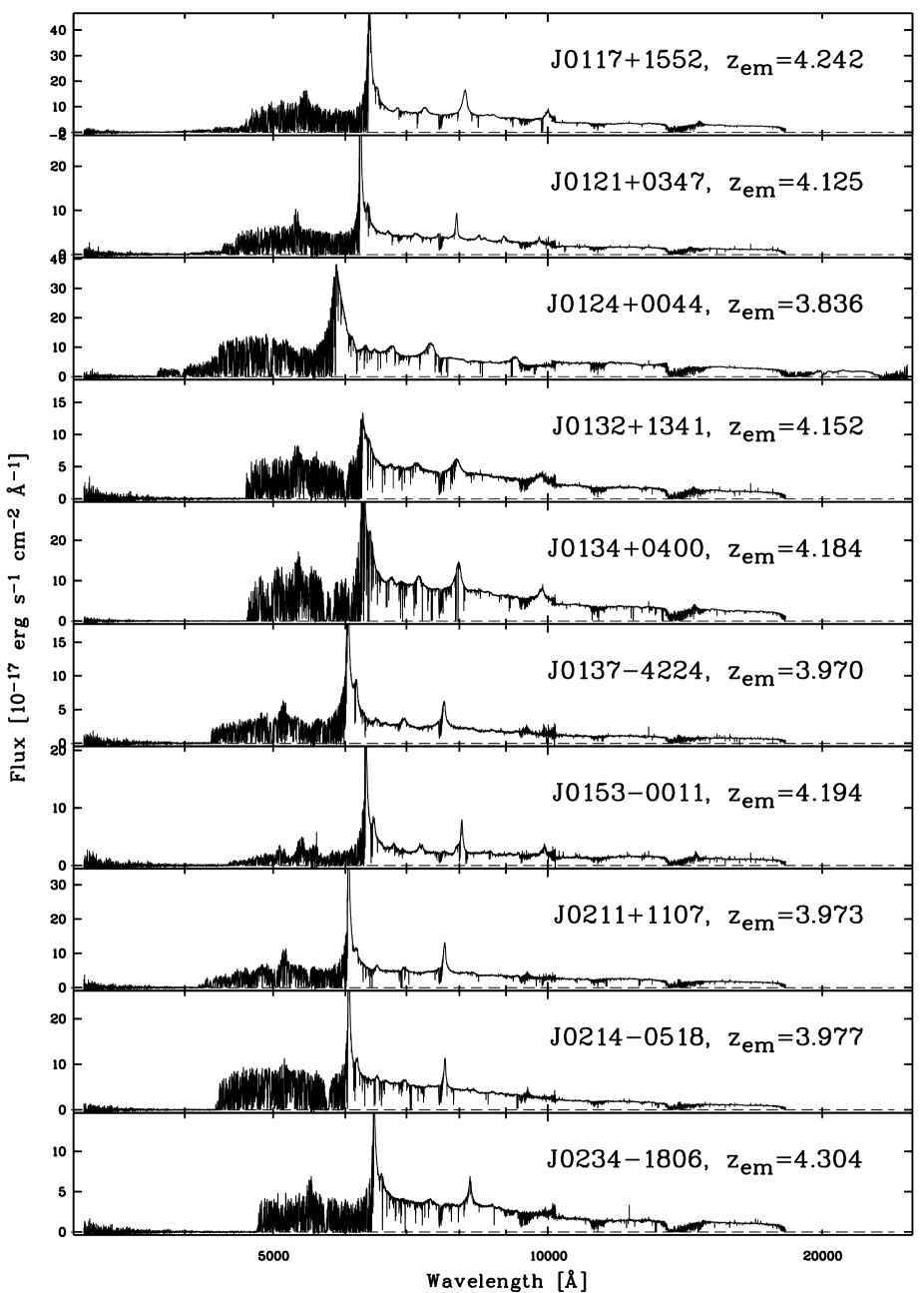
Figure 10: Same as Fig. 9.

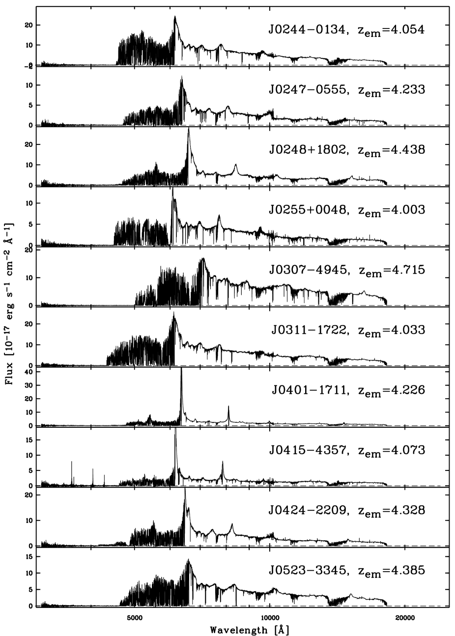
Figure 11: Same as Fig. 9.

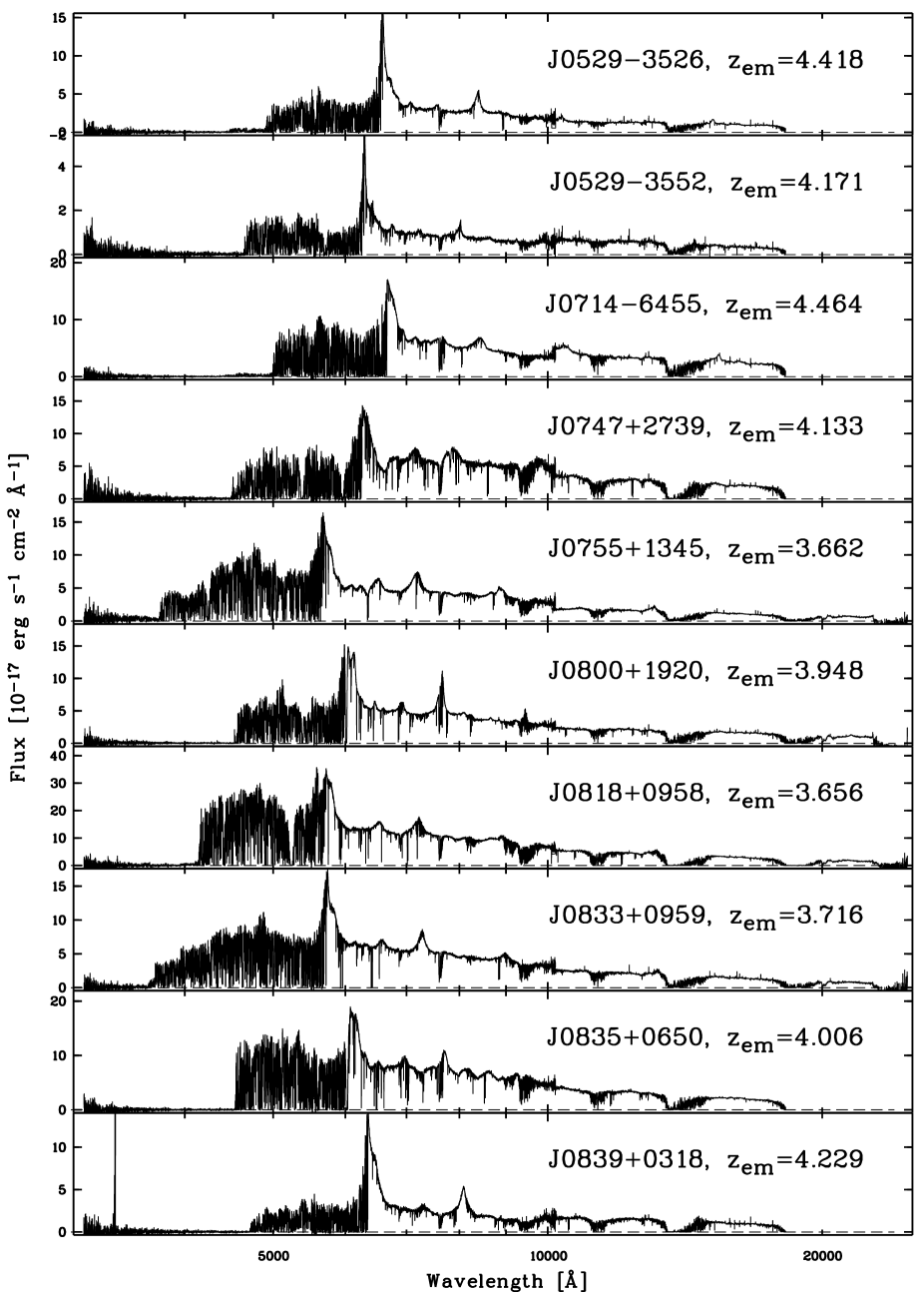
Figure 12: Same as Fig. 9.

Figure 13: Same as Fig. 9.

Figure 14: Same as Fig. 9.

Figure 15: Same as Fig. 9.

Figure 16: Same as Fig. 9.

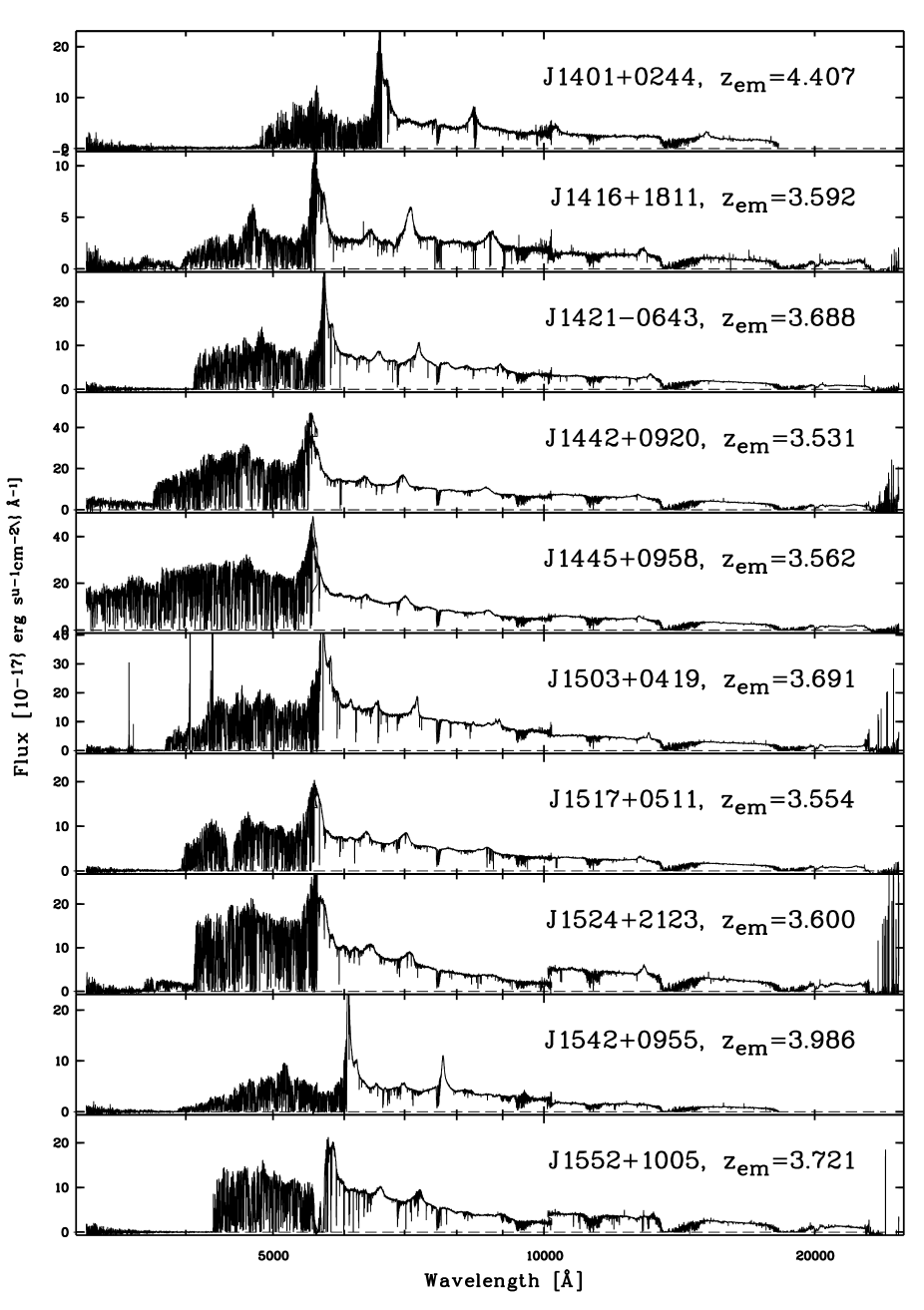
Figure 17: Same as Fig. 9.

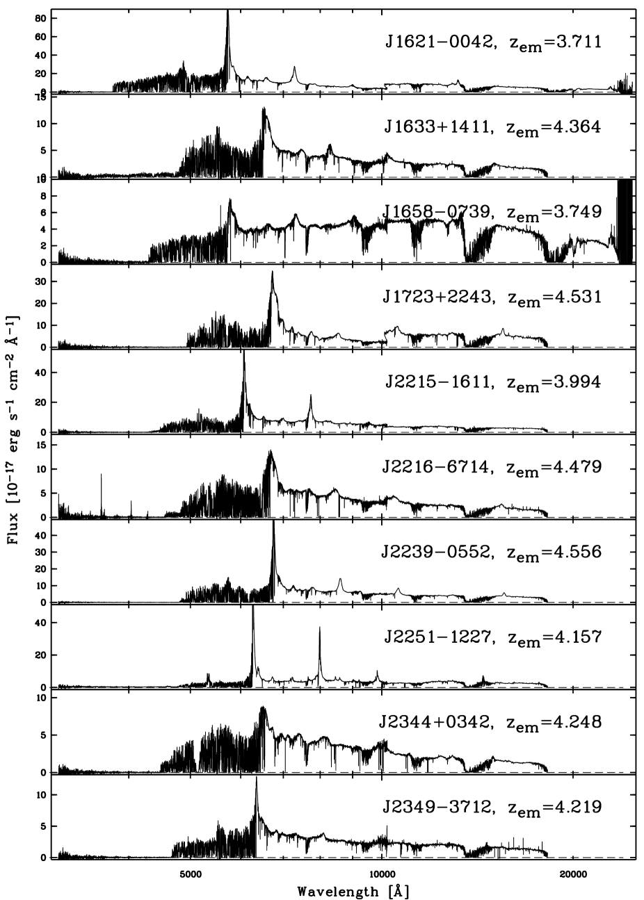
Figure 18: Same as Fig. 9.

References

- Aguirre et al. (2004) Aguirre, A., Schaye, J., Kim, T.-S., Theuns, T., Rauch, M. & Sargent, W. L. W. 2004 ApJ 602 38
- Alam et al. (2015) Alam, S., Albareti, F. D., Allende Prieto, C., et al. 2015, ArXiv:1501.00963
- Becker, Rauch & Sargent (2007) Becker, G. D., Rauch, M. & Sargent, W. L. W. 2007, ApJ, 662, 72
- Becker, Rauch & Sargent (2009) Becker, G. D., Rauch, M. & Sargent, W. L. W. 2009, ApJ, 698, 1010
- Becker et al. (2012) Becker, G. D., Sargent, W. L. W., Rauch, M., & Carswell, R. F. 2012, ApJ, 744, 91
- Becker et al. (2015) Becker, G. D., Bolton, J. S., Madau, P., Pettini, M., Ryan-Weber, E. V. & Venemans, B. P. 2015, MNRAS, 447, 3402
- Becker, White & Helfand (1995) Becker, R. H., White, R. L., & Helfand, D. J. 1995, ApJ, 450, 559
- Berg et al. (2016) Berg, T., Ellison, S. L., Sánchez-Ramírez, R. et al. et al. 2016, MNRAS, submitted.
- Bergeron et al. (2004) Bergeron J. et al. 2004, The Messenger, 118, 40
- Brunner et al. (2002) Brunner, R., Djorgovski, S. G., Prince, T. & Szalay, A., “Massive Data Sets in Astronomy”, in Handbook of Massive Data Sets, eds. J. Abello et al., Dordrecht: Kluwer Academic Publ., 2002, pp. 931-979.
- Calverley et al. (2011) Calverley, A. P., Becker, G. D., Haehnelt, M. G. & Bolton, J. S. 2011, MNRAS, 412, 2543
- Capellupo et al. (2015) Capellupo, D. M., Netzer, H., Lira, P., Trakhtenbrot, B. & Mejía-Restrepo, J. 2015, MNRAS. 446. 3427
- Chen et al. (2010) Chen, H.-W., Wild, V., Tinker, J. L., Gauthier, J.-R., Helsby, J. E., Shectman, S. A. & Thompson, I. B. 2010, ApJ 724, 176
- Croft et al. (2002) Croft, R. A. C., Weinberg, D. H., Bolte, M., Burles, S., Hernquist, L., Katz, N., Kirkman, D. & Tytler, D. 2002 ApJ, 581, 20
- Croft et al. (1998) Croft, R. A. C., Weinberg, D. H., Katz, N. & Hernquist, L. 1998, ApJ, 495, 44
- Cutri et al. (2003) Cutri, R. M., Skrutskie, M. F., van Dyk, S., et al. 2003, 2MASS All Sky Catalog of point sources.
- Dall’Aglio, Wisotzki & Worseck (2008) Dall’Aglio, A., Wisotzki, L. & Worseck, G. 2008, A&A, 491,465
- De Rosa et al. (2014) De Rosa, G., Venemans, B. P., Decarli, R., Gennaro, M., Simcoe, R. A., Dietrich, M., Peterson, B. M., Walter, F., Frank, S., McMahon, R. G., Hewett, P. C., Mortlock, D. J. & Simpson, Chris 2014, ApJ, 790, 145
- Djorgovski (2005) Djorgovski, S. G., “Virtual Astronomy, Information Technology, and the New Scientific Methodology”, in IEEE Proc. of CAMP05: Computer Architectures for Machine Perception, eds. V. Di Gesu & D. Tegolo, 2005, p. 125.
- D’Odorico et al. (2004) D’Odorico, V., Cristiani, S., Romano, D., Granato, G. L. & Danese, L. 2004, MNRAS, 351, 976
- D’Odorico et al. (2008) D’Odorico, V., Bruscoli, M., Saitta, F., Fontanot, F., Viel, M., Cristiani, S., & Monaco, P. 2008, MNRAS, 389, 1727
- D’Odorico et al. (2010) D’Odorico, V., Calura, F., Cristiani, S., & Viel, M. 2010, MNRAS, 401, 2715
- D’Odorico et al. (2013) D’Odorico, V., Cupani, G., Cristiani, S., Maiolino, R., Molaro, P., Nonino, M., Centurión, M., Cimatti, A., di Serego Alighieri, S., Fiore, F., Fontana, A., Gallerani, S., Giallongo, E., Mannucci, F., Marconi, A., Pentericci, L., Viel, M. & Vladilo, G. 2013, MNRAS, 435, 1198
- Dietrich et al. (2002) Dietrich, M., Appenzeller, I., Vestergaard, M., & Wagner, S. J. 2002, ApJ, 564, 581
- Dietrich et al. (2003) Dietrich, M., Hamann, F., Appenzeller, I. & Vestergaard, M., 2003 ApJ 596, 817
- Dietrich et al. (2009) Dietrich, M., et al., 2009, ApJ, 696, 1998
- Eisenstein et al. (2011) Eisenstein, D. J., Weinberg, D. H., Agol, E., et al. 2011, AJ, 142, 72
- Flesch (2015) Flesch, E. 2015, PASA, 32, 10
- Freudling et al. (2013) Freudling, W., Romaniello, M., Bramich, D. M., Ballester, P., Forchi, V., García-Dabló, C. E., Moehler, S. & Neeser, M. J. 2013, A&A, 559, 96
- Hamann & Ferland (1999) Hamann, F. & Ferland, G. 1999, ARA&A, 37, 487
- Hamann et al. (2002) Hamann, F., Korista, K. T., Ferland, G. J., Warner, C. & Baldwin, J. 2002, ApJ, 564, 592
- Ho et al. (2012) Ho, L. C., Goldoni, P., Dong, X., Greene, J. E. & Ponti, G. 2012, ApJ, 754, 11
- Horne (1986) Horne, K. 1986, PASP, 98, 609
- Iršič et al. (2016) Iršič, V., Viel, M., Berg, T. A. M., et al., MNRAS, submitted.
- Irwin, McMahon & Hazard (1991) Irwin, M., McMahon, R. G. & Hazard, C. 1991, ASPC, 21, 117
- Jiang et al. (2007) Jiang, L., Fan, X., Vestergaard, M., Kurk, J. D., Walter, F., Kelly, B. C. & Strauss, M. A. 2007, AJ, 134, 1150
- Jones et al. (2013) Jones, A., Noll, S., Kausch, W., Szyszka, C. & Kimeswenger, S. 2013, A&A, 560, 91
- Kelson (2003) Kelson, D. D. 2003, PASP, 115, 688
- Kim et al. (2002) Kim, T.-S., Carswell, R. F., Cristiani, S., D’Odorico, S., Giallongo, E. 2002 MNRAS, 335, 555
- Kirkman et al. (2003) Kirkman, D., Tytler, D., Suzuki, N., O’Meara, J. M. & Lubin, D. 2003 ApJS, 149, 1
- Kirkman et al. (2005) Kirkman, D., Tytler, D., Suzuki, N., Melis, C., Hollywood, S., James, K., So, G., Lubin, D., Jena, T., Norman, M. L. & Paschos, P. 2005, MNRAS, 360, 373
- Kondo et al. (2008) Kondo, S., et al. 2008, in Astronomical Society of the Pacific Conference Series, Vol. 399, Panoramic Views of Galaxy Formation and Evolution, ed. T. Kodama, T. Yamada, & K. Aoki, 209
- Ledoux et al. (2003) Ledoux, C., Petitjean, P. & Srianand, R. 2003 MNRAS, 346, 209
- Lu et al. (1996) Lu, L., Sargent, W. L. W., Barlow, T. A., Churchill, C. W. & Vogt, S. S. 1996 ApJS, 107, 475
- Marziani et al. (2009) Marziani, P., Sulentic, J. W., Stirpe, G. M., Zamfir, S. & Calvani, M. 2009, A&A, 495, 83
- Matejek & Simcoe (2012) Matejek, M. S., & Simcoe, R. A. 2012, ApJ, 761, 112
- Ménard et al. (2011) Ménard, B., Wild, V., Nestor, D., et al. 2011, MNRAS, 417, 801
- Molaro et al. (2013) Molaro, P., Centurión, M., Whitmore, J. B., Evans, T. M., Murphy, M. T., Agafonova, I. I., Bonifacio, P., D’Odorico, S., Levshakov, S. A., López, S., Martins, C. J. A. P., Petitjean, P., Rahmani, H., Reimers, D., Srianand, R., Vladilo, G. & Wendt, M. 2013 A&A, 555, 68
- Murphy, Webb & Flambaum (2003) Murphy, M. T., Webb, J. K. & Flambaum, V. V. 2003, MNRAS, 345, 609
- Noll et al. (2012) Noll, S., Kausch, W., Barden, M., Jones, A. M., Szyszka, C., Kimeswenger, S. & Vinther, J. 2012 A&A, 543, 92
- Noterdaeme et al. (2012a) Noterdaeme, P., Laursen, P., Petitjean, P., Vergani, S. D., Maureira, M. J., Ledoux, C., Fynbo, J. P. U., López, S. & Srianand, R. 2012a A&A 540, 63
- Noterdaeme et al. (2012b) Noterdaeme, P., Petitjean, P., Carithers, W. C., Pâris, I., Font-Ribera, A., Bailey, S., Aubourg, E., Bizyaev, D., Ebelke, G., Finley, H., Ge, J., Malanushenko, E., Malanushenko, V., Miralda-Escudé, J., Myers, A. D., Oravetz, D., Pan, K., Pieri, M. M., Ross, N. P., Schneider, D. P., Simmons, A. & York, D. G. 2012b, A&A, 547, L1
- O’Meara et al. (2015) O’Meara, J. M., Lehner, N., Howk, J. C., Prochaska, J. X., Fox, A. J., Swain, M. A., Gelino, C. R., Berriman, G. B. & Tran, H. 2015, AJ, 150, 111
- Palanque-Delabrouille et al. (2013) Palanque-Delabrouille, N. et al. 2013, A&A, 559, 85
- Pâris et al. (2012) Pâris, I., Petitjean, P., Aubourg, É., et al. 2012, A&A, 548, A66
- Pâris et al. (2014) Pâris, I., Petitjean, P., Aubourg, É., et al. 2014, A&A, 563, 54
- Patat & Hussain (2013) Patat, F. & Hussain, G. A. J. 2013, in Organizations, People and Strategies in Astronomy 2 (OPSA 2), ed. Heck, A., 231
- Peroux et al. (2011) Péroux, C., Bouché, N. Kulkarni, V. P., York, D. G. & Vladilo, G. 2011 MNRAS, 410, 2237
- Perrotta et al. (2016) Perrotta, S., D’Odorico, V., Prochaska, J. X., Cristiani, S., Cupani, G., Ellison, S. L., López, S., Becker, G. D., Berg, T. A. M., Christensen, L., Denney, K. D., Hamann, F., Pâris, I., Vestergaard, M. & Worseck, G. 2016, MNRAS, in press.
- Prochaska et al. (2003) Prochaska, J. X., Gawiser, E., Wolfe, A. M., Castro, S. & Djorgovski, S. G. 2003 ApJ, 595, 9
- Prochaska, Worseck & O’Meara (2009) Prochaska, J. X., Worseck, G. & O’Meara, J. M. 2009, ApJ, 705, 113
- Prochaska, O’Meara & Worseck (2010) Prochaska, J. X., O’Meara, J. M. & Worseck, G. 2010, ApJ, 718, 392
- Prochaska & Wolfe (2009) Prochaska, J. Xavier; Wolfe, Arthur M. 2009, ApJ, 696, 1543
- Rafelski et al. (2013) Rafelski, M. Wolfe, A. M., Prochaska, J. X., Neeleman, M. & Mendez, A. J. 2012, ApJ, 755, 89
- Rudie et al. (2012) Rudie, G. C., Steidel, C. C., Trainor, R. F., Rakic, O., Bogosavljević, M., Pettini, M., Reddy, N., Shapley, A. E., Erb, D. K. & Law, D. R. 2012 ApJ, 750, 67
- Ryan-Weber et al. (2009) Ryan-Weber, E. V., Pettini, M., Madau, P. & Zych, B. J. 2009, MNRAS, 395, 1476
- Sánchez-Ramírez et al. (2016) Sánchez-Ramírez, Ellison, S. L., Prochaska, J. X., Berg, T. A. M., López, S., D’Odorico, V., Becker, G. D., Christensen, L., Cupani, G., Denney, K. D., Pâris, I., Worseck, G. & Gorosabel, J. 2016, MNRAS, 456, 4488
- Scannapieco et al. (2006) Scannapieco, E., Pichon, C., Aracil, B., Petitjean, P., Thacker, R. J., Pogosyan, D., Bergeron, J. & Couchman, H. M. P. 2006, MNRAS, 365, 615
- Schaye et al. (2000) Schaye, J., Theuns, T., Rauch, M., Efstathiou, G. & Sargent, W. L. W. 2000, MNRAS, 318, 817
- Schneider et al. (2010) Schneider, D. P., Richards, G. T., Hall, P. B., et al. 2010, AJ, 139, 2360
- Simcoe et al. (2011) Simcoe, R. A., Cooksey, K. L., Matejek, M., Burgasser, A. J., Bochanski, J., Lovegrove, E., Bernstein, R. A., Pipher, J. L., Forrest, W. J., McMurtry, C., Fan, X. & O’Meara, J. 2011, ApJ, 743, 21
- Songaila (2005) Songaila, A. 2005 AJ, 130, 1996
- Songaila & Cowie. (2010) Songaila, A. & Cowie, L. L. 2010, ApJ, 721, 1448
- Srianand et al. (2004) Srianand, R., Chand, H., Petitjean, P. & Aracil, B. 2004, PhRvL, 92, 121302
- Storrie-Lombardi et al. (1994) Storrie-Lombardi, L. J., McMahon, R. G., Irwin, M. J. & Hazard, C. 1994, ApJ, 427, 13
- Sulentic et al. (2006) Sulentic, J. W., Repetto, P., Stirpe, G. M., Marziani, P., Dultzin-Hacyan, D., & Calvani, M. 2006, AAp, 456, 929 (Paper II)
- Sulentic et al. (2004) Sulentic, J. W., Stirpe, G. M., Marziani, P., Zamanov, R., Calvani, M., & Braito, V. 2004, AAp, 423, 121 (Paper I)
- Suzuki et al. (2005) Suzuki, N. and Tytler, D. and Kirkman, D. and O’Meara, J. M. and Lubin, D., 2005, ApJ, 618, 592
- Vernet et al. (2011) Vernet et al. 2011, A&A, 536A, 105
- Vestergaard & Peterson (2006) Vestergaard, M. & Peterson, B.M. 2006, ApJ, 641, 689
- Vestergaard & Osmer (2009) Vestergaard, M. & Osmer, P.S. 2009, ApJ, 699, 800
- Viel et al. (2004) Viel, M., Haehnelt, M. G., & Springel, V. 2004, MNRAS, 354, 684
- Viel et al. (2009) Viel, M., Bolton, J. S., & Haehnelt, M. G. 2009, MNRAS, 399, L39
- Viel et al. (2013) Viel, M., Becker, G. D., Bolton, J. S. & Haehnelt, M. G. 2013, PhRvD, 88, 043502
- Worseck & Prochaska (2011) Worseck, G. & Prochaska, J. X. 2011, ApJ, 728, 23
- Worseck et al. (2014) Worseck, G., Prochaska, J. X., O’Meara, J. M., Becker, G. D., Ellison, S. L., López, S., Meiksin, A., Ménard, B., Murphy, M. T. & Fumagalli, M. 2014 MNRAS, 445, 1745
- Wright et al. (2010) Wright, E. L., Eisenhardt, P. R. M., Mainzer, A. K., et al. 2010, AJ, 140, 1868
- Wolfe, Gawiser & Prochaska (2005) Wolfe, A. M., Gawiser, E. & Prochaska, J. X. 2005, ARA&A, 43, 861
- York et al. (2000) York, D. G., Adelman, J., Anderson, Jr., J. E., et al. 2000, AJ, 120, 1579
- Zafar et al. (2013) Zafar, T., Popping, A. & Péroux, C. 2013, A&A, 556, A140
- Zhu & Ménard (2013) Zhu, G. & Ménard, B. 2013, ApJ, 770, 130
- Zuo et al. (2015) Zuo, W., Wu, X-B., Fan, X., Green, R., Wang, R. & Bian, F. 2015, ApJ, 799, 189