Semi-supervised evidential label propagation algorithm for graph data

Abstract

In the task of community detection, there often exists some useful prior information. In this paper, a Semi-supervised clustering approach using a new Evidential Label Propagation strategy (SELP) is proposed to incorporate the domain knowledge into the community detection model. The main advantage of SELP is that it can take limited supervised knowledge to guide the detection process. The prior information of community labels is expressed in the form of mass functions initially. Then a new evidential label propagation rule is adopted to propagate the labels from labeled data to unlabeled ones. The outliers can be identified to be in a special class. The experimental results demonstrate the effectiveness of SELP.

1 Introduction

With the increasing size of networks in real world, community detection approaches should be fast and accurate. The Label Propagation Algorithm (LPA) [5] is known to be one of the near-linear solutions and benefits of easy implementation, thus it forms a good basis for efficient community detection methods. The behavior of LPA is not stable because of the randomness. Different communities may be detected in different runs over the same network. Moreover, by assuming that a node always adopts the label of the majority of its neighbors, LPA ignores any other structural information existing in the neighborhood.

Semi-supervised classification has been widely studied for classical data sets, but there has been little work on semi-supervised community detection. In many scenarios a substantial amount of prior knowledge about the graph structure may be available. It can reflect the application-specific knowledge about cluster membership to some extent. For instance, in a co-authorship community network, it may be possible to label a small subset of scholars based on their research interests. In a social network application, it may be desirable to label some nodes according to their affinity to some products.

In [4] the authors considered the individual labels as prior knowledge, i.e. the true community assignments of certain nodes are known in advance. In their work the traditional LPA is adapted, allowing a few nodes to have true community labels, but the rest nodes are unlabeled. In face the presented semi-supervised community detection approach is an application of the semi-supervised classification algorithm proposed by [7] on graph data sets.

In this paper, we enhance the original LPA by introducing new update and propagation strategies using the theory of belief functions. The Semi-supervised version of Evidential Label Propagation (SELP) algorithm is presented. SELP can take advantage of the limited amount of supervised information and consequently improve the detection results.

The remainder of this paper is organized as follows. Some basic knowledge is briefly introduced in Section 2. The SELP algorithm is presented in detail in Section 3. In order to show the effectiveness of the proposed community detection approach, in Section 4 SELP algorithm is tested on different graph data sets. Conclusions are drawn in the final section.

2 Background

In this section some related preliminary knowledge will be presented. Some basis of belief function theory will be recalled first. As this work is inspired from the LPA [5] and E$K$-NNclus [2] clustering, the two algorithms will also be briefly introduced.

2.1 Theory of belief functions

Let $\Omega=\{\omega_{1},\omega_{2},\ldots,\omega_{c}\}$ be the finite domain of $X$, called the discernment frame. The belief functions are defined on the power set $2^{\Omega}=\{A:A\subseteq\Omega\}$.

The function $m:2^{\Omega}\rightarrow[0,1]$ is said to be the Basic Belief Assignment (bba) on $2^{\Omega}$, if it satisfies:

$$\sum_{A\subseteq\Omega}m(A)=1.$$ (1)

Every $A\in 2^{\Omega}$ such that $m(A)>0$ is called a focal element. The credibility and plausibility functions are defined in Eqs.$~{}\eqref{bel}$ and $\eqref{pl}$ respectively:

$$Bel\text{(}A\text{)}=\sum_{B\subseteq A,B\neq\emptyset}m\text{(}B\text{)}~{}~{}\forall A\subseteq\Omega,$$ (2)

$$Pl\text{(}A\text{)}=\sum_{B\cap A\neq\emptyset}m\text{(}B\text{)},~{}~{}\forall A\subseteq\Omega.$$ (3)

Each quantity $Bel(A)$ measures the total support given to $A$, while $Pl(A)$ represents potential amount of support to $A$.

If bbas $m_{j},j=1,2,\cdots,S$ describing $S$ distinct items of evidence on $\Omega$, the DS rule of combination [6] of $S$ bbas can be mathematically defined as

$$(m_{1}\oplus m_{2} \oplus\cdots\oplus m_{S})(X)=$$

$$\begin{cases}0&\text{if}~{}X=\emptyset,\\ \frac{\sum\limits_{Y_{1}\cap\cdots\cap Y_{S}=X}\prod_{j=1}^{S}m_{j}(Y_{j})}{1-\sum\limits_{Y_{1}\cap\cdots\cap Y_{S}=X}\prod_{j=1}^{S}m_{j}(Y_{j})}&\text{otherwise}.\end{cases}$$ (4)

2.2 E$K$-NNclus clustering

Recently, a new decision-directed clustering algorithm for relational data sets, named E$K$-NNclus, is put forward based on the evidential $K$ nearest-neighbor (E$K$-NN) rule [2]. Starting from an initial partition, the algorithm, called E$K$-NNclus, iteratively reassigns objects to clusters using the E$K$-NN rule [1], until a stable partition is obtained. After convergence, the cluster membership of each object is described by a mass function assigning a mass to each specific cluster and to the whole set of clusters.

2.3 Label propagation

Let $G(V,E)$ be an undirected network, $V$ is the set of $N$ nodes, $E$ is the set of edges. Each node $v(v\in V)$ has a label $c_{v}$. Denote by $N_{v}$ the set of neighbors of node $v$. The Label Propagation Algorithm (LPA) uses the network structure alone to guide its process. It starts from an initial configuration where every node has a unique label. Then at every step one node (in asynchronous version) or each node (in a synchronous version) updates its current label to the label shared by the maximum number of its neighbors. For node $v$, its new label can be updated to $\omega_{j}$ with

$$j=\arg\max_{l}\{|u:c_{u}=l,u\in N_{v}|\},$$ (5)

where $|X|$ is the cardinality of set $X$, and $N_{v}$ is the set of node $v$’s neighbors. When there are multiple maximal labels among the neighbors’ labels, the new label is picked randomly from them. By this iterative process densely connected groups of nodes form consensus on one label to form communities, and each node has more neighbors in its own community than in any of other community. Communities are identified as a group of nodes sharing the same label.

3 Semi-supervised label propagation

Inspired from LPA and E$K$-NNclus [2], we propose here SELP algorithm for graph data sets with prior information. The problem of semi-supervised community detection will be first described in a mathematical way, and then the proposed SELP algorithm will be presented in detail.

3.1 Problem restatement and notions

Let $G(V,E)$ denote the graph, where $V$ is the set of $n$ nodes and $E\subseteq V\times V$ is the set of edges. Generally, a network can be expressed by its adjacent matrix $\bm{A}=(a_{ij})_{n\times n}$, where $a_{ij}=1$ indicates that there is a direct edge between nodes $i$ and $j$, and 0 otherwise.

Assume that there are $c$ communities in the graph. The set of labels is denoted by $\Omega=\{\omega_{1},\omega_{2},\cdots,\omega_{c}\}$. In addition, in order to make sure that the solution is unique, we assume that there must be at least one labeled vertex in each community. The $n$ nodes in set $V$ can be divided into two parts:

$$V_{L}=\{(n_{1},y_{1}),(n_{2},y_{2}),\cdots,(n_{l},y_{l})\},~{}~{}y_{j}\in\Omega$$

for the labeled nodes, and

$$V_{U}=\{n_{l+1},n_{l+2},\cdots,n_{n}\}$$

for the unlabeled ones. The main task of the semi-supervised community detection is to make models propagating the labels from nodes in $V_{L}$ to those in $V_{U}$, and further determine the labels of those unlabeled vertices.

3.2 The dissimilarities between nodes

Like the smooth assumption in the semi-supervised graph-based learning methods [8], here we assume that the more common neighbors the two nodes share, the larger probability that they belong to the same community. Thus in this work, the index considering the number of shared common neighbors is adopted to measure the similarities between nodes.

Definition 1. Let the set of neighbors of node $n_{i}$ be $N_{i}$, and the degree of node $n_{i}$ be $d_{i}$. The similarity between nodes $n_{i}$ and $n_{j}$ ($n_{i},n_{j}\in V$) is defined as

$$s_{ij}=\begin{cases}\frac{|N_{i}\cap N_{j}|}{d_{i}+d_{j}},&~{}\text{if}~{}a_{ij}=1\\ 0,&~{}\text{otherwise}.\end{cases}$$ (6)

Then the dissimilarities associated with the similarity measure can be defined as

$$d_{ij}=\frac{1-s_{ij}}{s_{ij}},~{}\forall~{}n_{i},n_{j}\in V.$$ (7)

3.3 Evidential label propagation

For a labeled node $n_{j}\in V_{L}$ in community $\omega_{k}$, the initial bba can be defined as a Bayesian categorical mass function:

$$m^{j}(A)=\begin{cases}1&~{}\text{if}~{}A=\{\omega_{k}\}\\ 0&~{}\text{otherwise}.\end{cases}$$ (8)

For an unlabeled node $n_{x}\in V_{U}$, the vacuous mass assignment can be used to express our ignorance about its community label:

$$m^{x}(A)=\begin{cases}1&~{}\text{if}~{}A=\Omega\\ 0&~{}\text{otherwise}.\end{cases}$$ (9)

To determine the label of node $n_{x}$, its neighbors can be regarded as distinct information sources. If there are $|N_{x}|=r_{x}$ neighbors for node $n_{x}$, the number of sources is $r_{x}$. The reliability of each source depends on the similarities between nodes. Suppose that there is a neighbor $n_{t}$ with label $\omega_{j}$, it can provide us with a bba describing the belief on the community label of node $n_{x}$ as [2]

$$m_{t}^{x}(\{\omega_{t}\}) =\alpha*m^{t}(\{\omega_{j}\}),$$

$$m_{t}^{x}(\Omega) =m^{t}(\Omega)+(1-\alpha)*m^{t}(\{\omega_{j}\}),$$

$$m_{t}^{x}(A) =0,~{}~{}\text{if}~{}A\neq\{\omega_{j}\},\Omega,$$ (10)

where $\alpha$ is the discounting parameter such that $0\leq\alpha\leq 1$. It should be determined according to the similarity between nodes $n_{x}$ and $n_{t}$. The more similar the two nodes are, the more reliable the source is. Thus $\alpha$ can be set as a decreasing function of $d_{xt}$. In this work we suggest to use

$$\alpha=\alpha_{0}\exp\{-\gamma d_{xt}^{\beta}\},$$ (11)

where parameters $\alpha_{0}$ and $\beta$ can be set to be 1 and 2 respectively as default, and $\gamma$ can be set to

$$\gamma=1/\text{median}\left(\left\{d_{ij}^{\beta},~{}i=1,2,\cdots,n,~{}j\in N_{i}\right\}\right).$$ (12)

After the $r_{x}$ bbas from its neighbors are calculated using Eq. (3.3), the fused bba of node $n_{x}$ can be got by the use of Dempster’s combination rule:

$$m^{x}=m_{1}^{x}\oplus m_{2}^{x}\oplus\cdots\oplus m_{r_{x}}^{x}.$$ (13)

The label of node $n_{x}$ can be determined by the maximal value of $m^{x}$. The main principle of semi-supervised learning is to take advantage of the unlabeled data. It is an intuitive way to add node $n_{x}$ (previously in set $V_{U}$ but already be labeled now) to set $V_{l}$ to train the classifier. However, if the predicted label of $n_{x}$ is wrong, it will have very bad effects on the accuracy of the following predictions. Here a parameter $\eta$ is introduced to control the prediction confidence of the nodes that to be added in $V_{l}$. If the maximum of $m^{x}$ is larger than $\eta$, it indicates that the belief about the community of node $n_{x}$ is high and the prediction is confident. Then we remove node $n_{x}$ in $V_{U}$ and add it to set $V_{L}$. On the contrary, if the maximum of $m^{x}$ is not larger than $\eta$, it means that we can not make a confident decision about the label of $n_{x}$ based on the current information. Thus the node $n_{x}$ should be remained in set $V_{U}$. This is the idea of self-training [3].

In order to propagate the labels from the labeled nodes to the unlabeled ones in the graph, a classifier should be first trained using the labeled data in $V_{l}$. For each node $n_{x}$ in $V_{U}$, we find its direct neighbors and construct bbas through Eq. (3.3). Then the fused bba about the community label of node $n_{x}$ is calculated by Eq. (13). The subset of the unlabeled nodes, of which the maximal bba is larger than the given threshold $\eta$, are selected to augment the labeled data set. The predicted labels of these nodes are set to be the class assigned with the maximal mass. Parameter $\eta$ can be set to 0.7 by default in practice.

After the above update process, there may still be some nodes in $V_{U}$. For these nodes, we can find their neighbors that are in $V_{L}$, and then use Eqs. (3.3) and (13) to determine their bbas.

4 Experiment

In order to verify the efficiency and effectiveness of the proposed SELP algorithm, some experiments on graph data sets will be conducted in this section, and the results by the use of different methods will be reported. The semi-supervised community detection algorithm using label propagation (SLP) [4] and the unsupervised label propagation algorithm will be used to compare the performance. The parameters in SELP are all set to the default values in the experiments.

4.1 Real world networks

A. Karate Club network. In this experiment we tested on the widely used benchmark in detecting community structures, “Karate Club”. The network consists of 34 nodes and 78 edges representing the friendship among the members of the club. During the development, a dispute arose between the club’s administrator and instructor, which eventually resulted in the club split into two smaller clubs. The first one was an instructor-centered group covering 16 vertices: 1–-8, 11-–14, 17-–18, 20 and 22, while the second administrator centered group consisted of the remaining 18 vertices.

Figure 1: Karate Club network.

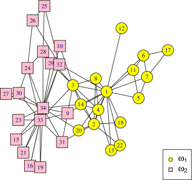
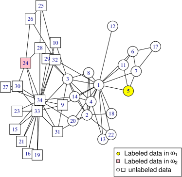
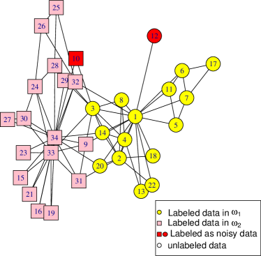
In the first test, the labeled node in community $\omega_{1}$ was set to node 5, while that in community $\omega_{2}$ was set to node 24. After five steps, SELP algorithm stopped. The detailed update process is displayed in Figure 2. It can be seen from the figure that two outliers, nodes 10 and 12 are detected by SELP. From the original graph, we can see that node 10 has two neighbors, nodes 3 and 34. But neither of them shares a common neighbor with node 10. For node 12, it only connects to node 1, but has no connection with any other node in the graph. Therefore, it is very intuitive that both the two nodes are regarded as outliers of the graph.

The detection results on Karate Club network by SELP and SLP algorithms with different labeled nodes are shown in Table 1. The labeled vertices and its corresponding misclassified vertices are clearly presented in the table. As can be seen from the table, nodes 10 and 12 are detected as outliers in all the cases by SELP, and the two communities can be correctly classified most of the time. The performance of SLP is worse than that of SELP when there is only one labeled data in each community. For the nodes which are connected to both communities and located in the overlap, such as nodes 3 and 9, they are misclassified most frequently. If the number of labeled data in each community is increased to 2, the exact community structure can be got by both methods. It is indicated that the more prior information (i.e. labeled vertices) we have, the better the performance of SELP is.

a. Initialization

b. $it=5$

Figure 2: The results on Karate Club network. The nodes marked with color red are the outliers detected by SELP.

Table 1: Community detection results for the Karate Club network.

Labeled nodes in $\omega_{1}$	Labeled nodes in $\omega_{2}$	Misclassified nodes by SELP	Detected outliers by SELP	Misclassified nodes by SLP
1	34	None	10, 12	None
1	32	9	10, 12	9, 10, 27, 31, 34
2	33	None	10, 12	None
6	31	3	10, 12	2, 3, 8, 14, 2
8	31	None	10, 12	10
8	32	None	10, 12	None
17	31	3, 4, 8, 14	10, 12	2, 3, 4, 8, 13, 14, 18, 20, 22
1, 2	33, 34	None	10, 12	None
1, 2	33, 9	None	10, 12	None
3, 18	26, 30	None	10, 12	None
17, 4	31, 9	None	10, 12	None

B. American football network. As a further test of our algorithm, the network we investigated in this experiment was the world of American college football games.

a. Error rate

b. NMI

Figure 3: The results on American football network. The two figures show the average error rates and NMI values (plus and minus one standard deviation) for 50 repeated experiments, as a function of the number of labeled samples.

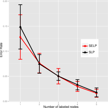
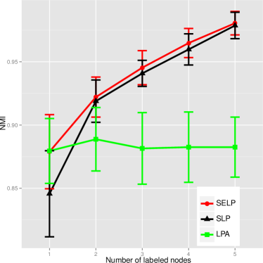
Let the number of labeled nodes in each community to be fixed. Then SELP and SLP algorithms were evoked 50 times respectively with randomly selected labeled nodes. The average error rates and NMI values (plus and minus one standard deviation) of the 50 experiments are displayed in Figures 3-a and 3-b respectively. As can be seen from the figures, with the increasing number of labeled samples, the performance of both SELP and SLP becomes better. The NMI values of the detected communities by SELP and SLP are significantly better than those by LPA. It indicates that the semi-supervised community detection methods could take advantage of the limited amount of prior information and consequently improve the accuracy of the detection results. The behavior of SELP is better than that of SLP in terms of both error rates and NMI values.

4.2 LFR network

In this subsection, LFR benchmark networks were used to test the ability of the algorithm to identify communities. The experiments here included evaluating the performance of the algorithm with various amounts of labeled nodes and different values of parameter $\mu$ in the benchmark networks. The original LPA [5] and the semi-supervised community detection approach SLP [4] were used to compare.

In LFR networks, the mixing parameter $\mu$ represents the ratio between the external degree of each vertex with respect to its community and the total degree of the node. The larger the value of $\mu$ is, the more difficult the community structure will be correctly detected. The values of the parameters in LFR benchmark networks in this experiment were set as follows: $n=1000,\xi=15,\tau_{1}=2,\tau_{2}=1,cmin=20,cmax=50$.

a. Error rate

b. NMI

Figure 4: The results on LFR network. The number of labeled nodes in each community is 3.

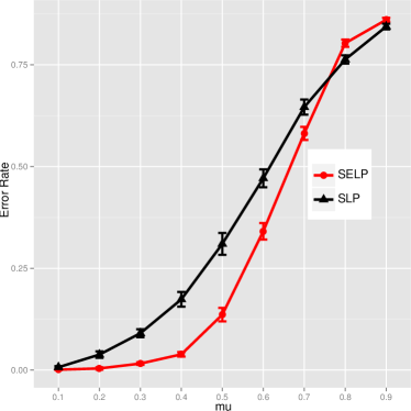
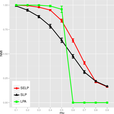
The performance of different methods with various values of $\mu$ is shown in Figure 4. As expected, the error rate is very high and the NMI value is low when $\mu$ is large. It demonstrates the fact that the community structure is not very clear and consequently difficult to be identified correctly. It can be seen from Figure 4-a that the error rates by SELP are smaller than those by SLP generally. SELP performs better than SLP. This conclusion could also be got in terms of the NMI values displayed in Figure 4-b.

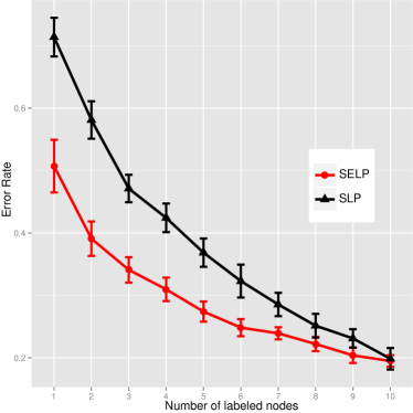
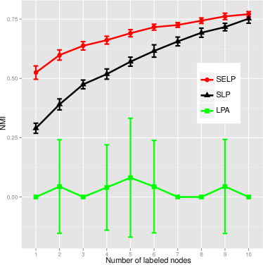
The original LPA could not work at all when $\mu$ is larger than 0.5. The results of SELP and SLP are significantly improved in these cases compared with LPA. As shown in Figure 5-b, even when there is only one labeled data in each community, the behavior of SELP is much better than that of LPA. This confirms the fact that the semi-supervised community detection approaches can effectively take advantage of the limited amount of labeled data. From Figure 5, we can also see that the performance of SELP and SLP becomes better with the increasing number of labeled nodes.

a. Error rate

b. NMI

Figure 5: The results on LFR network. The parameter of $\mu$ is set to be 0.6.

5 Conclusion

In this paper, the semi-supervised evidential label propagation algorithm is presented as an enhanced version of the original LPA. The proposed community detection approach can effectively take advantage of the limited amount of supervised information. This is of practical meaning in real applications as there often exists some prior knowledge for the analyzed graphs. The experimental results show that the detection results will be significantly improved with the help of limited amount of supervised information.

References

- [1] Denœux, T.: A -nearest neighbor classification rule based on dempster-shafer theory. Systems, Man and Cybernetics, IEEE Transactions on 25(5), 804–813 (1995)
- [2] Denœux, T., Kanjanatarakul, O., Sriboonchitta, S.: EK-NNclus: A clustering procedure based on the evidential -nearest neighbor rule. Knowledge-Based Systems 88, 57–69 (2015)
- [3] Li, M., Zhou, Z.H.: SETRED: Self-training with editing. In: Advances in Knowledge Discovery and Data Mining, pp. 611–621. Springer (2005)
- [4] Liu, D., Bai, H.Y., Li, H.J., Wang, W.J.: Semi-supervised community detection using label propagation. International Journal of Modern Physics B 28(29), 1450208 (2014)
- [5] Raghavan, U.N., Albert, R., Kumara, S.: Near linear time algorithm to detect community structures in large-scale networks. Physical Review E 76(3), 036106 (2007)
- [6] Shafer, G.: A mathematical theory of evidence. Princeton University Press (1976)
- [7] Wang, F., Zhang, C.: Label propagation through linear neighborhoods. Knowledge and Data Engineering, IEEE Transactions on 20(1), 55–67 (2008)
- [8] Zhu, X., Lafferty, J., Rosenfeld, R.: Semi-supervised learning with graphs. Carnegie Mellon University, language technologies institute, school of computer science (2005)