Black hole accretion discs and screened scalar hair

Abstract

We present a novel way to investigate scalar field profiles around black holes with an accretion disc for a range of models where the Compton wavelength of the scalar is large compared to other length scales. By analysing the problem in “Weyl” coordinates, we are able to calculate the scalar profiles for accretion discs in the static Schwarzschild, as well as rotating Kerr, black holes. We comment on observational effects.

DCPT-16/25

1 Introduction

In modern cosmology, we are well aware we have to find a compelling explanation for the late time acceleration of the universe – one that fits not only observation [1, 2, 3, 4, 5, 6], but also is theoretically consistent. One intriguing possibility is that of a light rolling scalar field. From a purely theoretical point of view, massless scalar fields or moduli are abundant in string and supergravity theories: Generic string compactifications result in a plethora of massless scalars in the low energy $4D$ effective theory, including Kaluza-Klein scalars describing the size of the compactified dimension; distances between branes in brane-world type scenarios appear as scalar fields, and in addition to this, any supergravity theory requires scalar counterparts to all fermionic degrees of freedom thus $\mathcal{N}\geq 4$ supergravity necessarily contains scalars in the gravity multiplets.

All of the above seems to suggest that adding scalars to the low energy description of gravity might be a reasonable thing to do. However, a famous theorem due to Weinberg [7] shows that any such modification necessarily introduces a new dynamical degree of freedom which in turn produces a fifth force. If the mediator of this force is light (which is necessary for the field to be of cosmological relevance) it would lead to unacceptably large violations of the Equivalence Principle (EP) within the solar system.Therefore if the reason for the late time acceleration of the universe is a scalar, there must be a mechanism to screen out its EP-violating effects.

To explore such screening mechanisms, one schematically writes the scalar Lagrangian as

$${\cal L}\supset\frac{Z(\phi_{o})}{2}(\partial\delta\phi)^{2}-\frac{m^{2}(\phi_{o})}{2}(\delta\phi)^{2}+\frac{\gamma(\phi_{o})}{M_{\text{Pl}}}\delta\phi T$$ (1.1)

where small variations of the scalar $\delta\phi$ around the background value $\phi_{o}$ can couple to the trace of the energy momentum tensor $T$. We can now see qualitatively the various different screening scenarios: The scalar force is screened by the Vainshtein mechanism when $Z(\phi_{o})$ is large enough that the canonically normalised field coupling, $\gamma(\phi_{o})/Z^{1/2}(\phi_{o})$, is small. The chameleon mechanism [8, 9] occurs when the mass $m(\phi_{o})$ is large enough to suppress the range of the scalar force. The symmetron [10] and dilaton [11] screenings work by suppressing the scalar coupling $\gamma(\phi_{o})$. In all of these cases, the background value of the field $\phi_{o}$ depends on the environment and the screening mechanisms occur in the presence of dense matter.

Obviously these theories have been scrutinised heavily in the laboratory [12, 13, 14, 15, 16, 17], solar system [18], astrophysical [19, 20], and cosmological [21, 22] settings (see also [23] and [24] for interesting recent commentary on the cosmological chameleon). All of these investigations, however, probe gravity in a regime where the gravitational fields and space-time curvatures are relatively weak. After the direct detection of gravitational waves from LIGO [25], we can now hope that gravitational waves from compact binary systems will allow us to constrain the behaviour of gravity in the strong field, large curvature regime. Accordingly, attention has increasingly focussed on efforts to test gravity by studying the dynamics of compact objects such as neutron stars and black holes, [26, 27], and thus it is natural to ask whether observations of black holes might provide new constraints on screened modified gravity [28, 29, 30].

The constraints from pulsar systems [31] rely on the fact that in scalar-tensor theories neutron stars take on a non-constant scalar profile, producing equivalence principle violations. In the context of black holes and additional scalar degrees of freedom, however, the uniqueness of exact solutions needs to be carefully examined due a number of “no-hair” theorems that require the scalar fields to take on a constant value around isolated black holes [32, 33, 35, 34]. This might seem to imply that black hole systems will not be useful for constraining screened modified gravity. However all of these no-hair theorems generally apply to black hole systems that are asymptotically flat, stationary, and include no matter – hardly the typical galactic environment! By systematically relaxing these assumptions we can gain insight into scenarios where screened modified gravity may have non-trivial effects on black hole dynamics.

Indeed, even without modifying gravity, there are many interesting phenomena with scalars and non-static black holes. For example, unstable massive scalar modes around rotating black holes [38, 39, 37, 40, 41, 36], or scalar hair around rotating black holes in Einstein gravity [42, 44, 43]. It has also been shown that scalar hair will be induced if the asymptotic boundary conditions for the scalar field vary slowly with time [47, 48, 46, 45] (see also [49] for a study of spherical collapse in scalar-tensor gravity). This time variation, which violates the conditions of stationarity and asymptotic flatness, could be due to either the cosmological evolution of the scalar field’s background value or to the motion of the black hole through an external scalar gradient. Referencing this, [46] has used observations of a black hole binary to constrain the cosmological time dependence for extremely light scalar fields. The numerical calculations presented in [50] also support this idea by showing that black holes moving through a non-uniform scalar gradient can emit scalar monopole and dipole radiation, and [51, 52] explore other possible observational effects of scalar hair.

In a previous paper, [53], we made a preliminary investigation using an artificial matter distribution around a black hole – an ‘accretion’ thick sphere that extended from $r=6GM$ out to large $r$ in a Schwarzschild black hole. The purpose of that investigation was to first establish, within the rules of the no hair theorems, that a black hole could indeed support scalar hair. Next, analytic modelling of the scalar profile was undertaken and compared in detail with numerical solutions so that we could confidently make an estimate of the magnitude of the scalar profile for a generic scalar model. Finally, using this data, we explored and estimated observational effects. Our aim here is to revisit the crude (and unrealistic) model for the accretion sphere of the black hole, and to use a more realistic disc model, and explore to what extent the results we derived previously were dependent on the assumed matter distribution around the black hole.

This paper is organised as follows: we briefly review screened modified gravity in §2. Next we solve for the scalar profile around a Schwarzschild black hole with an accretion disc in §3 followed by the Kerr black hole in §4 and conclude by commenting on possible implications in §5.

2 Screened modified gravity

The way we solve the scalar equation of motion requires the scalar to evolve slowly (to be made more precise later) in response to the non-uniform matter density of an accretion disc. While several screening mechanisms exist, we focus on the frameworks where the additional scalar degree of freedom is constrained to have a large Compton wavelength compared to the length scale of astrophysical black holes. As we argued in [53], this is a common feature in several of the most popular screening mechanisms including the chameleon, the environmentally dependent dilaton, and the symmetron.

The basic idea of screening is that the scalar mass or the coupling to matter (or both) is dependent on the local energy density, hence in a dense environment such as our solar system, the field becomes ‘heavy’, effectively decouples, and thus no fifth force modifications of gravity are present in such environments. On the other hand, at cosmological scales and densities, the field is light and can give rise to modifications of the gravitational interaction.

The relevant models of screened modified gravity include: the chameleon mechanism, [8, 9], which occurs when the mass of the scalar field, $m(\phi_{0})$, is large enough to suppress the range of the scalar force; the environmental dilaton, [11], where the coupling function between the scalar and matter fields and the mass alter in dense regions; and the symmetron, [10], where the coupling function switches off in dense environments. These mechanisms can be modelled generically with the Einstein frame action

$$S=\int d^{4}x\sqrt{-g}\left[-\frac{M_{p}^{2}}{2}R+\frac{1}{2}g^{\mu\nu}\partial_{\mu}\phi\partial_{\nu}\phi-V(\phi)\right]+S_{m}\left[\Psi_{i},A^{2}(\phi)g_{\mu\nu}\right].$$ (2.1)

Where $M_{p}^{2}=1/8\pi G$ gives the Planck mass, $S_{m}$ represents the matter action (denoted generically as $\Psi_{i}$), and $A(\phi)$ is the conformal coupling between the Einstein and Jordan frames $\tilde{g}_{\mu\nu}=A^{2}(\phi)g_{\mu\nu}$. The details of a particular theory are completely specified by the scalar potential $V(\phi)$ and the coupling function $A(\phi)$.

Using this set-up, and identifying a conserved density $\rho\equiv-A^{-1}T_{m}$ in the Einstein frame [54], the scalar equation of motion becomes

$$\square\phi=\frac{\partial}{\partial\phi}\left[V(\phi)+(A(\phi)-1)\rho\right]\equiv\frac{\partial V_{\text{eff}}(\phi,\rho)}{\partial\phi}.$$ (2.2)

Thus we see explicitly the density-dependent effective potential $V_{\text{eff}}(\phi,\rho)$ that is the source of the screening behaviour for chameleons, environmentally dependent dilatons, and symmetrons.

3 Schwarschild Black Hole

We start by exploring the accretion disc around a Schwarzschild black hole, as a warm up for the full Kerr problem. In order to proceed, we require a simple model for the physical set-up. We assume that we have some background ambient density field, ignoring for now any general isotropic build up of matter in the neighbourhood of the black hole. Superposed on this ambient density field is the accretion disc, which is generally highly concentrated in the equatorial plane, extending out from the Innermost Stable Circular Orbit (ISCO) of the black hole.

We model the accretion disc by a uniform density $\delta-$function on the equatorial plane extending from the ISCO to some (arbitrary) outer radius $r_{1}$ characteristic of the accretion disc or the galactic plane. This has the desirable property of being disc-like and constrained in a 2-dimensional plane around the black hole, although the constant density profile is an idealisation. Astrophysically realistic accretion disc models involve complex fluid dynamics typically requiring numerical modelling (see [55] for a detailed review) and are beyond the scope of this work. However our results should capture the salient features of these more involved models, have the particular benefit of being amenable to analytic analysis, and should provide a reasonable estimate for the scalar field profiles.

The idea is to analyse the scalar equation (2.2) in the strongly curved geometry near the black hole event horizon for this idealised disc source. Our aim is to proceed as far as possible analytically, so that we can obtain general results and features of the solution that can be used in a wider range of models than if we were to pick specific potentials, couplings, and solve the problem numerically.

The first step is to choose an appropriate coordinate system for the analysis. As we will see, it turns out to be most rewarding to rewrite the Schwarzschild metric in “Weyl” form, where the radial and polar angles $\{r,\theta\}$ are re-badged as a pair of cartesian-like coordinates $\{x,y\}$ such that the $x-y$ part of the metric is conformally flat:

$$ds^{2}=e^{2\lambda}dt^{2}-e^{2(\nu-\lambda)}\left(dx^{2}+dy^{2}\right)-\alpha^{2}e^{-2\lambda}d\varphi^{2}$$ (3.1)

This is the general Weyl metric form, but for the Schwarzschild solution, the functions take the form

$$\alpha\equiv x\;,\qquad\lambda={\frac{1}{2}}\ln{X_{+}-Y_{+}\over X_{-}-Y_{-}}\;,\qquad\nu={1\over 2}\ln{(X_{+}X_{-}+Y_{+}Y_{-}+x^{2})\over 2X_{+}X_{-}}$$ (3.2)

with

$$Y_{\pm}=y\pm GM\qquad,\qquad X_{\pm}^{2}=x^{2}+Y_{\pm}^{2}$$ (3.3)

We can return to the familiar $\{r,\theta\}$ Schwarzschild coordinates via the transformation

$$x^{2}=r(r-2GM)\sin^{2}\theta\;\;,\;\;\;y=(r-GM)\cos\theta$$ (3.4)

Now consider the scalar field equation in this background. Our model for the accretion disc supposes that while it may have highly nontrivial local dynamics, these average out to an approximately uniform density profile strongly localised in the equatorial plane. The scalar profile therefore will be dependent essentially on only the radial and polar coordinates. This is the reason for choosing this less well known Weyl coordinate system for the Schwarzschild metric – the wave operator turns out to have a simple form if the scalar depends only on $x$ and $y$, being proportional to a flat-space cylindrical Laplacian, leading to the equation of motion for $\phi$:

$$\Box\phi\equiv\frac{1}{\sqrt{-g}}\partial_{\mu}\left(\sqrt{-g}g^{\mu\nu}\partial_{\nu}\right)\phi=e^{-2(\nu-\lambda)}\left[\frac{1}{x}\frac{\partial~{}}{\partial x}\left(x\frac{\partial\phi}{\partial x}\right)+\frac{\partial^{2}\phi}{\partial y^{2}}\right]=\frac{\partial V_{\text{eff}}(\phi,\rho)}{\partial\phi}$$ (3.5)

for the appropriate $V_{\text{eff}}$.

In [53], we used a much simpler background matter density in the vicinity of the black hole, and found approximate analytical solutions, comparing them to full numerical solutions for the scalar profile. With the exception of long Compton wavelength symmetrons, these were largely similar, with screened scalars having broadly similar profiles that peaked near the event horizon. We will therefore consider the Chameleon model in this paper, and take a large Compton wavelength compared to the typical black hole length scales. The current experimentally constrained model parameters of environmentally dependent dilatons and symmetrons also put them in the same category of long Compton wavelength scalars.

In the chameleon models, it is typically assumed that the coupling function is to a good approximation an exponential:

$$A(\phi)=e^{\beta\phi/M_{p}},$$ (3.6)

where $\beta$ is nearly constant over the range of field values of interest. In addition, a typical chameleon potential is usually taken to be

$$V(\phi)=M^{4+n}\phi^{-n}=V_{0}\phi^{-n},$$ (3.7)

where $n\geq 1$ is an integer of order one, and we define $V_{0}\equiv M^{4+n}$ to simplify notation. Keeping only the leading order term from the coupling function, we see that the effective potential is

$$V_{\text{eff}}(\phi,\rho)\approx\frac{V_{0}}{\phi^{n}}+\frac{\rho\beta\phi}{M_{p}},$$ (3.8)

minimised at

$$\phi_{\text{min}}^{n+1}=\frac{nV_{0}M_{p}}{\rho\beta}.$$ (3.9)

The mass of small fluctuations of the field around this minimum is

$$m^{2}(\rho) =\left.V_{\text{eff}}(\phi,\rho),_{\phi\phi}\right|_{\phi_{\text{min}}}$$ (3.10)

$$\approx\frac{\rho\beta}{M_{p}}\left[(n+1)\left(\frac{\rho\beta}{nV_{0}M_{p}}\right)^{\frac{1}{n+1}}+\frac{\beta}{M_{p}}\right]$$

which, as required, increases monotonically with $\rho$.

To find $\rho$, note that in the Weyl coordinates the equatorial plane corresponds to $y=0$, and the ISCO radius, $r=6GM$ for the Schwarzschild black hole, corresponds to $x_{0}=2\sqrt{6}GM_{BH}=\sqrt{6}r_{s}$, where $r_{s}=2GM_{BH}$ is the Schwarzschild radius. Thus the accretion disc model we are using has the density profile

$$\rho\rightarrow\rho_{0}+\rho_{1}\delta(y)\Theta[x-x_{0}]\Theta[x_{1}-x]$$ (3.11)

in Weyl coordinates.

We now make two simplifying assumptions in order to explore scalar solutions analytically. Firstly, we use this crude model for the disc (3.11). Secondly, we assume that the solution for the scalar is dominated by the effect of $\rho_{1}$, the accretion disc itself; essentially this means we expand our scalar around $\phi_{\text{min}}$

$$\phi\sim\phi_{\text{min}}+\delta\phi$$ (3.12)

where $\phi_{\text{min}}$ is the background scalar field profile due to the ambient background density $\phi_{0}$. Finally, we assume that the mass of the scalar is negligible. This will be a good approximation within the Compton radius of the scalar, and provided our system does not extend over many Compton wavelengths, should give a realistic picture for the scalar profile.

Making these assumptions, (3.5) reduces to a Poisson equation for $\delta\phi$:

$$(x\delta\phi_{,x})_{,x}+x\delta\phi_{,yy}=\frac{\beta\rho_{1}(\mathbf{r})}{M_{p}}\,xe^{2(\nu-\lambda)}$$ (3.13)

for which we can use the massless scalar Green’s function to obtain:

$$\delta\phi=-\frac{\beta}{4\pi M_{p}}\int d^{3}\mathbf{r^{\prime}}\frac{\rho_{1}(\mathbf{r^{\prime}})e^{2(\nu-\lambda)}}{\lvert\mathbb{r}-\mathbb{r^{{}^{\prime}}}\lvert}$$ (3.14)

The accretion disc model (3.11) localises this integral to the equatorial plane where

$$e^{2(\nu-\lambda)}\mid_{y^{\prime}=0}=\frac{(\sqrt{4x^{\prime 2}+r_{s}^{2}}+r_{s})^{2}}{4x^{\prime 2}+r_{s}^{2}}$$ (3.15)

and using

$$\int^{\pi}_{-\pi}\frac{d\varphi^{\prime}}{\sqrt{y^{2}+x^{2}+x^{\prime 2}-2xx^{\prime}\cos(\varphi-\varphi^{\prime})}}=\frac{4}{\sqrt{(x+x^{\prime})^{2}+y^{2}}}\;\text{K}\left[\frac{4xx^{\prime}}{(x+x^{\prime})^{2}+y^{2}}\right]$$ (3.16)

where K is the complete elliptic integral of the first kind, $\delta\phi$ becomes

$$\delta\phi=-\frac{\beta\rho_{1}r_{s}}{\pi M_{p}}\int^{x_{1}}_{x_{0}}\frac{(\sqrt{4x^{\prime 2}+r_{s}^{2}}+r_{s})^{2}}{x^{\prime 2}+r_{s}^{2}}\;\text{K}\left[\frac{4xx^{\prime}}{(x+x^{\prime})^{2}+y^{2}}\right]\;\frac{x^{\prime}dx^{\prime}}{\sqrt{y^{2}+(x+x^{\prime})^{2}}}$$ (3.17)

Once we specify an $x_{1}$, we can integrate up this expression to obtain $\delta\phi$, which we will do presently. However, for the moment we would like to obtain an order of magnitude estimate for $\delta\phi$, and its dependence on the various parameters analytically. First, extract the dependence on the black hole mass by rescaling $\hat{x}=x/GM_{BH}=2x/r_{s}$:

$$\delta\phi=-\frac{\beta\rho_{1}r_{s}^{2}}{4M_{p}}\;{\hat{\delta\phi}}=-\frac{\beta\rho_{1}r_{s}^{2}}{4\pi M_{p}}\;{\cal{I}}[\hat{x},\hat{y}]$$ (3.18)

where

$${\cal{I}}[\hat{x},\hat{y}]=\int^{\hat{x}_{1}}_{2\sqrt{6}}\left(\frac{(\sqrt{\hat{x}^{\prime 2}+1}+1)^{2}}{\hat{x}^{\prime 2}+1}\right)\;\text{K}\left[\frac{4\hat{x}\hat{x}{{}^{\prime}}}{(\hat{x}+\hat{x}^{\prime})^{2}+\hat{y}^{2}}\right]\;\frac{\hat{x}^{\prime}d\hat{x}^{\prime}}{\sqrt{\hat{y}^{2}+(\hat{x}+\hat{x}^{\prime})^{2}}}$$ (3.19)

The prefactor in (3.17) gives the parameter dependence for the scalar, and we now approximate (3.19) to get an estimate of the order of magnitude of $\hat{\delta\phi}$.

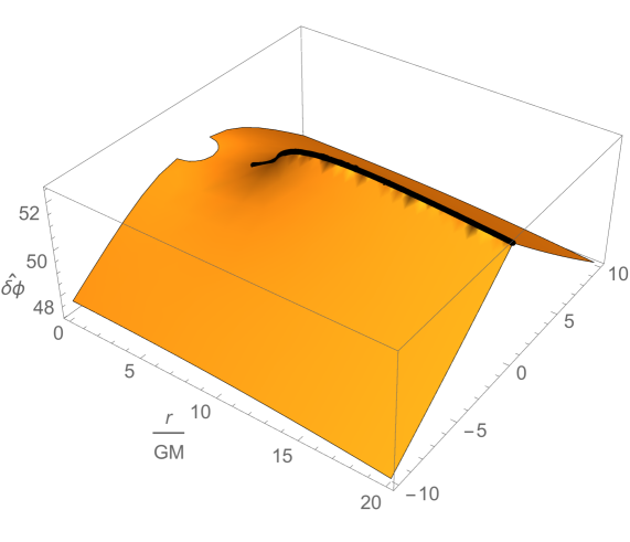
Figure 1: 3D plot illustrating the (normalised) scalar field profile $\hat{\delta\phi}$ around the Schwarzschild accretion disc. The start of the accretion disc (shown as a thick black line) can be clearly seen around $x\approx 5$.

The first term for ${\cal I}$ in brackets is monotonically decreasing, and for $\hat{x}^{\prime}\geq 2\sqrt{6}$ lies in the range $[1,36/25]$, thus we approximate this term by $1$. The elliptic function is roughly $\pi/2$ unless $\hat{y}\approx 0$, $\hat{x}\approx\hat{x}^{\prime}$, i.e., on the accretion disc, however since the singularity of K is logarithmic, this will not give a huge enhancement to the integral, thus we approximate this contribution to the integrand by $\pi/2$. This leaves us with the final term, that can be integrated exactly to give

$${\cal I}[\hat{x},\hat{y}]\simeq\frac{\pi}{2}\left[R_{1}-R_{0}-\hat{x}\ln\frac{\hat{x}+\hat{x}_{1}+R_{1}}{\hat{x}+\hat{x}_{0}+R_{0}}\right]$$ (3.20)

where we have written $R_{i}=\sqrt{(\hat{x}+\hat{x}_{i})^{2}+y^{2}}$ for clarity. Expanding this at large $\hat{r}=\sqrt{\hat{x}^{2}+\hat{y}^{2}}$ gives ${\cal I}\approx\pi(\hat{x}_{1}^{2}-\hat{x}_{0}^{2})/2\hat{r}$, i.e. the expected “$1/r$” fall-off of a massless field. Near the black hole and disc, $\hat{x}\approx\hat{x}_{0},\hat{y}\approx 0$, and ${\cal I}\approx\pi\hat{x}_{1}/2$. We therefore obtain an order of magnitude estimate for the magnitude of the chameleon near the disc of:

$$\delta\phi\approx-\frac{\beta\rho_{1}r_{s}^{2}}{8M_{p}}\;\frac{r_{1}}{r_{s}}$$ (3.21)

Note that this will be an underestimate, since in each case in the integrand, our estimate was the lower, though more consistent, value of the function. At large distances from the disc, the profile becomes very accurate, but closer in, we may expect some discrepancy.

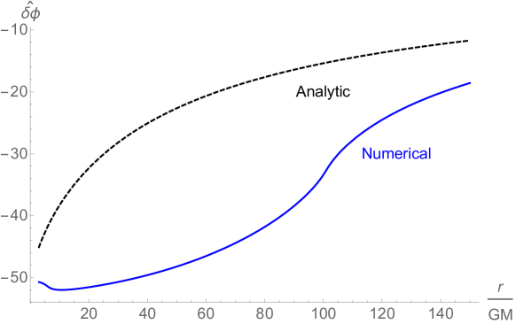
Figure 2: A comparison of the analytic (under)estimate and the numerically integrated result plotted in Schwarzschild ‘cartesians’, $(r\sin\theta,r\cos\theta)$, at constant $r\cos\theta=GM$. The largest disparity between the two curves is along the length of the accretion disc ($6GM<r<100GM$), with the curves approaching at larger $r$. The peak estimate for $\delta\phi$ agrees within $10\%$ however.

In order to check this estimate, we integrated (3.19) using mathematica; figure 1 shows the scalar field plotted in Schwarzschild coordinates $(r\sin\theta/GM,r\cos\theta/GM)$, and figure 2 shows the accuracy (or otherwise) of this estimate. The presence of the accretion disc clearly causes the scalar field to respond and lifts it from its ambient background value. The disc itself is evident in the plot from the sharp crease in the profile, resulting from the integrated singularity of the elliptic function. This is clearly an artefact of the fact we have modelled the disc with a hard $\delta-$function profile. In a more realistic scenario, the accretion disc while strongly localised near $y=0$, will have some spread on either side, and we would expect this kink discontinuity to smooth out.

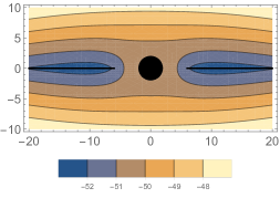
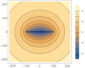
Figure 3: Comparison of near field and far field fall off around the Schwarzschild accretion disc, indicated in each plot by the horizontal thick black line.

On large distances, the scalar rolls back to its ambient value, as expected from the physics and analytic approximation. Figure 3 shows the near and further field solutions for $\delta\phi$. In practise, once the scalar Compton wavelength scale is reached, the field will then transition to the typical exponential fall-off expected of the massive field profile.

It is interesting to query to what extent the scalar profile is due to the geometry of the black hole, and what to the matter distribution, which would in any case cause the scalar to shift. Figure 4 shows a comparison of the scalar perturbation from the disc plus black hole, to the disc only. This clearly shows that primary feature of the scalar being pulled from its equilibrium value by the dense matter is due to the disc matter density, however, the black hole does impact on the magnitude of the effect (if one looks at the contour values) increasing it by about $10\%$. On the one hand, this might suggest that the black hole is not that relevant, however, the disc would obviously not be there without the black hole to drive it. In addition this confirms the fact that in spite of the strong gravity regime of the black hole, and the notion that the event horizon is somehow “special”, the scalar still behaves and responds to its environment, with the black hole providing a marginal boost to the local matter environment effects. As a result, it seems counter-intuitive that a black hole would behave differently towards a scalar than the local galactic medium, as suggested for example for Vainstein screening [56].

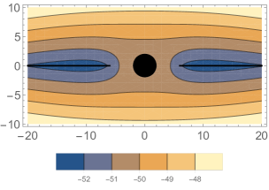
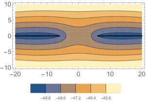
Figure 4: Comparison of scalar profile with and without a black hole. The disc profile is taken to have the same form, starting at $r=6GM$, and ending at $r=100GM$.

4 Kerr Geometry

Having discussed the static, spherically symmetric case it is now surprisingly straightforward to turn to the more physically interesting case of the rotating Kerr geometry, usually written in spherical polar Boyer-Lindquist coordinates as

$$ds^{2}=\frac{\Delta-a^{2}\sin^{2}\theta}{\Sigma}dt^{2}+\frac{4GMar\sin^{2}\theta}{\Sigma}dtd\varphi-\frac{\beta}{\Sigma}\sin^{2}\theta d\varphi^{2}-\frac{\Sigma}{\Delta}dr^{2}-\Sigma d\theta^{2}$$ (4.1)

where $a=J/M$ and

$$\Sigma =r^{2}+a^{2}\cos^{2}\theta$$ (4.2)

$$\Delta =r^{2}-2GMr+a^{2}$$

$$\Gamma =(r^{2}+a^{2})^{2}-\Delta a^{2}\sin^{2}\theta$$

Following the method described for the simpler Schwarzschild geometry, we begin by rewriting the metric in Weyl coordinates [57]

$$ds^{2}=e^{2\lambda}dt^{2}-\alpha^{2}e^{-2\lambda}[d\varphi+Bdt]^{2}-e^{2(\nu-\lambda)}(dx^{2}+dy^{2})$$ (4.3)

where

$$x\equiv\alpha=\sqrt{\Delta}\sin\theta\;\;,\quad y=(r-GM)\cos\theta$$ (4.4)

To get the Weyl functions, we first define

$$Y_{\pm} =y\pm\sqrt{G^{2}M^{2}-a^{2}},$$ (4.5)

$$X^{2}_{\pm} =x^{2}+y^{2}_{\pm}\qquad\Rightarrow\quad X_{\pm} =r-GM\pm\sqrt{G^{2}M^{2}-a^{2}}\cos\theta$$

Giving

$$e^{2\lambda}=\frac{\Delta\Sigma}{\Gamma}\;\;,\quad B=\frac{2aGMr}{\Gamma}\;\;,\quad e^{2(\nu-\lambda)}=\frac{\Sigma}{X_{+}X_{-}}$$ (4.6)

where

$$r=\frac{X_{+}+X_{-}}{2}+GM\;\;,\quad\cos\theta=\frac{X_{+}-X_{-}}{2\sqrt{G^{2}M^{2}-a^{2}}}$$ (4.7)

Once again, we model the accretion disc by the simplified energy distribution (3.11), and insert in (3.13) now the Kerr measure

$$e^{2(\nu-\lambda)}\mid_{y=0}=\frac{(\sqrt{\hat{x}^{\prime 2}+1-\hat{a}^{2}}+1)^{2}}{\hat{x}^{\prime 2}+1-\hat{a}^{2}}$$ (4.8)

where, as before, we have rescaled our Weyl coordinates, and $\hat{a}=a/GM_{BH}\in[0,1]$.

It is easy to see that the scalar equation of motion remains mostly unaffected by the addition of rotation into the geometry. Its functional form is unchanged in Weyl coordinates, although the multiplicative factor of $e^{2(\lambda-\nu)}$ must now take the Kerr form. The general expression (3.17) therefore remains the same, with $r_{s}=2GM_{BH}$ representing now the black hole mass rather than the horizon radius, and with the integral function replaced by the appropriately modified Kerr expression:

$${\cal{I}}_{\text{Kerr}}[\hat{x}_{1}]=\int^{\hat{x}_{1}}_{\hat{x}_{0}}\left(\frac{(\sqrt{\hat{x}^{\prime 2}+1-\hat{a}^{2}}+1)^{2}}{\hat{x}^{\prime 2}+1-\hat{a}^{2}}\right)\;\text{K}\left[\frac{4\hat{x}\hat{x}{{}^{\prime}}}{(\hat{x}+\hat{x}^{\prime})^{2}+\hat{y}^{2}}\right]\;\frac{\hat{x}^{\prime}d\hat{x}^{\prime}}{\sqrt{\hat{y}^{2}+(\hat{x}+\hat{x}^{\prime})^{2}}}$$ (4.9)

where $\hat{x}_{0}$ is the rescaled ISCO value of $x$. The general expression for $\hat{x}_{0}$ in terms of $\hat{a}$ is somewhat unwieldy, however, the key feature is that $\hat{x}_{0}$ decreases as $\hat{a}$ increases, eventually merging with the event horizon at $\hat{x}_{0}=0$.

As before, the elliptic integral contributes roughly a constant, except very near the accretion disc where is gives a slight uplift to the integral. The final term is unchanged, however, the first factor, coming from the $e^{2(\nu-\lambda)}$ term, is now potentially rather different if the black hole is at, or very near, extremality. For $\hat{a}\sim 1$, this term is roughly $1/\hat{x}^{\prime 2}$, and thus the integral generically diverges logarithmically as $\hat{x}_{\text{ISCO}}\to 0$ in the extremal limit, with a linear divergence at $\hat{x}=\hat{y}=0$. Although this sounds alarming, because of the precipitous drop in the ISCO as $a\to a_{\text{ext}}$, $x_{\text{ISCO}}\sim 2^{\frac{2}{3}}(1-\hat{a})^{\frac{1}{3}}$, this only contributes an uplift to ${\cal{I}}_{\text{Kerr}}$ of order a few for any realistic astrophysical black hole. We therefore expect a very similar expression to (3.20) for an estimate of the integral. The primary difference will be that the strongest shift of the scalar will be near the ISCO, which will be much closer to the event horizon of the black hole, therefore correspondingly a sharper profile. This is borne out by the numerical integrations shown in figure 5, which show the scalar profile in Boyer-Lindquist coordinates for $\hat{a}=0.5$ and $0.95$.

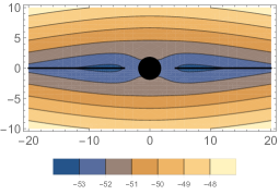
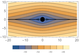
Figure 5: The normalized scalar profile $\hat{\delta\phi}$ plotted in cartesian coordinates for increasing rotation: $a/GM=0.5,0.95$. The accretion disc is represented as a solid black line and the black hole as a black circle in the middle.

Our overall conclusion therefore is that the disc pulls the scalar from its ambient value to a central order of magnitude of (3.21). Rotating black holes give a stronger effect, but only by about $5-10\%$, even for a nearly extreme black hole.

5 Summary and Discussion

In the main part of this paper, we presented an analytic analysis of the scalar profile around a Schwarzschild or Kerr black hole with an accretion disc. With the assumption of a very sharp profile accretion disc, modelled by a $\delta-$function, the scalar depends only on the radial distance and angle from the rotation axis. Using the less-well known Weyl co-ordinate system for the black hole geometry, the scalar equation of motion simplifies considerably to a form for which a Green’s function is known. We used this to estimate analytically the scalar field profile, then confirmed this by a simple numerical integration.

The scalar has a nontrivial profile around the black hole, and is ‘pinned’ to its largest value on the accretion disc, very near the ISCO. The main result is the scalar displacement amplitude (3.21):

$$\delta\phi=-\frac{\beta\rho_{1}r_{s}^{2}}{8M_{p}}\;{\cal{I}}$$ (5.1)

where ${\cal I}=r_{1}/r_{s}$ represents the extent of the dense accretion flow. We now turn to a discussion of the potential astrophysical consequences and observable effects of this scalar profile. Our initial assumptions about the accretion disc being a small addition, so as to not disrupt the background Schwarzschild or Kerr geometry appreciably, would guarantee the magnitude of any effect due to the scalar field to be small.

The most obvious effect to consider would be an additional fifth force felt by any test particle in the vicinity of the black hole accretion disc system. Though it is entirely possible that these additional forces would cause the structure of the accretion disc to be non-trivially modified, such effects would require astrophysical modelling beyond the scope of the present work. We considered this possibility in [53], where we concluded that the effect would be too small to be observed for a coupling $\beta$ of $O(1)$ and while the magnitude of the scalar is similar here since the modelling of the accretion disk is rather different we should be able to get a better estimate of the fifth force.

The effects of the scalar gradient on a test particle can easily be estimated as the ratio of the fifth force to the Newtonian force is

$$\frac{|F_{\phi}|}{|F_{N}|}\approx\left(\frac{r}{r_{s}}\right)^{2}\beta(\phi)|\vec{\nabla}\phi|\frac{M_{BH}}{M_{p}^{3}}.$$ (5.2)

(5.1) allows us to approximate this as

$$10^{-11}\beta^{2}{\cal{I}}\lesssim\frac{|F_{\phi}|}{|F_{N}|}\lesssim 10^{-3}\beta^{2}{\cal{I}}$$ (5.3)

where we use $\rho_{1}\sim 10^{21}\rho_{cos}$, $\vec{\nabla}\phi\sim\delta\phi/R_{1}$ and $M_{BH}\sim 10^{6}-10^{10}M_{\odot}\sim 10^{44}-10^{48}M_{p}$ We note that while this ratio is small, for $\beta\sim\mathcal{O}(10-10^{2})$, which is an allowed parameter range for the chameleon model [17], the effects could be an appreciable percentage of the Newtonian force in some cases.

It is obvious from the force estimation that to evaluate the relevance of our scalar field profile in the accretion disk, we should compare the emission of any scalar radiation to gravitational radiation. We can do this if we view our static black hole model as the supermassive partner of an extreme mass ratio inspiral (EMRI) binary system. Such EMRI systems typically consist of a stellar mass compact object orbiting a supermassive black hole and in GR they emit gravitational radiation at a rate approximated to leading order in $\dot{r}$ by the quadrupole formula. Comparing this to the scalar radiation gives,

$$\left|\frac{\dot{\mathcal{E}}_{\phi}}{\dot{\mathcal{E}}_{GR}}\right|\sim\beta\left(\frac{R_{0}}{R_{s}}\right)^{\frac{9}{2}}\left(\frac{\delta\phi}{\delta r}\right)\frac{M_{BH}}{M_{p}^{3}}\left[\frac{M_{BH}}{m_{t}}\right].$$ (5.4)

Where $m_{t}$ is a test mass. For $m_{t}\sim M_{\odot}$ and

$$10^{6}\leq\frac{M_{BH}}{M_{\odot}}\leq 10^{10}$$ (5.5)

we get,

$$\beta^{2}10^{-5}\lesssim\left|\frac{\dot{\mathcal{E}}_{\phi}}{\dot{\mathcal{E}}_{GR}}\right|\lesssim\beta^{2}10^{7}$$ (5.6)

For ultramassive black holes the ratio of scalar to gravitational radiation is very large. Since observations of such objects are currently rare we do not know if the fate of stellar mass inspirals would be similar to those in supermassive black holes. It would be interesting to see if such scalar radiation emitted by inspirals could be observed.

Another interesting effect which could potentially be observable is a shift in the atomic spectra. The scalar field in the chameleon model couples to matter and therefore the effective mass of elementary particles within the accretion disk will now receive a small correction proportional to $\delta\phi$ [58]. For the electron we have,

$$m_{e}(\phi)=m_{e}(1+\frac{\delta\phi}{M_{p}})$$ (5.7)

This in turn should add a correction to all atomic spectra. In particular it will change the Balmer and Lyman $\alpha$ series via an effect on the Rydberg constant and as it turns out both of these are observable in the quasar spectra, see eg SDSS [59]. The Rydberg constant, in natural units, may be expressed as,

$$R_{\infty}=\frac{\alpha^{2}m_{e}}{4\pi}$$ (5.8)

where $\alpha$ is the fine structure constant. The shift in the energy levels, assuming a correction to just the Rydberg constant, is then

$$\frac{\Delta E}{E}=\frac{\delta\phi}{M_{p}}$$ (5.9)

since $\delta\phi$ is negative this gives a negative shift in the energy levels of order

$$\beta 10^{-13}<\left|\frac{\Delta E}{E}\right|<\beta 10^{-5}$$ (5.10)

The shift is the same for the $H_{\alpha}$, $H_{\beta}$ and $Ly_{\alpha}$ lines. It remains to be seen whether or not this can be detected with future surveys, though for $\beta\sim\mathcal{O}(10)$ the shift could be appreciable for supermassive black holes.

If the scalar couples to photons via loop effects [60] then there will be a shift in hyperfine splitting as well. However, this is beyond the scope of this paper and requires further investigation. Such hyperfine splitting would be easier to distinguish from the spectral lines required to determine the quasar redshift.

Our results are also strongly indicative of a breakdown of the no-hair theorems when applied to realistic astrophysical black holes. The presence of a small amount of matter surrounding the black hole is enough to violate the stringent conditions required for the no-hair theorems to be valid and as such their use in breaking the model degeneracy between various modified gravity scenarios would be very limited .

It has previously been argued that black holes and stars in the centre of galaxies would behave differently under the effect of the additional scalar force because, while the star will feel the effects of such a force, the black hole would be protected by a no-hair theorem [56, 35]. Our results show that this is not the case and that in any realistic astrophysical scenario the situation is likely to be much more complex and the effects of the accretion disk has to be taken into account when computing the force experienced by an astrophysical black hole in the centre of a galaxy compared to that experienced by the stars. This is beyond the scope of this investigation.

References

- [1] S. Perlmutter et al., Measurements of and from 42 High Redshift Supernovae, The Astrophysical Journal 517 (June, 1999) [astro-ph/9812133].
- [2] A. G. Riess et al., Observational Evidence from Supernovae for an Accelerating Universe and a Cosmological Constant, The Astronomical Journal 116 (Sept., 1998) [astro-ph/9805201].
- [3] D. N. Spergel et al. [WMAP Collaboration], First year Wilkinson Microwave Anisotropy Probe (WMAP) observations: Determination of cosmological parameters, Astrophys. J. Suppl. 148, 175 (2003) [astro-ph/0302209].
- [4] SDSS Collaboration, K. N. Abazajian et al., The Seventh Data Release of the Sloan Digital Sky Survey, Astrophys. J. Suppl. 182 (2009) 543–558, [arXiv:0812.0649 [astro-ph]].
- [5] WMAP Collaboration, G. Hinshaw et al., Nine-Year Wilkinson Microwave Anisotropy Probe (WMAP) Observations: Cosmological Parameter Results, The Astrophysical Journal Supplement, Volume 208, Issue 2, 25 pp. (2013) [arXiv:1212.5226 [astro-ph]].
- [6] Planck Collaboration, P. Ade et al., Planck 2013 results. XVI. Cosmological parameters, Astron. Astrophys. 571, A16 (2014) [arXiv:1303.5076 [astro-ph]].
- [7] S. Weinberg, The Cosmological Constant Problem, Rev. Mod. Phys. 61, 1 (1989).
- [8] J. Khoury and A. Weltman, Chameleon cosmology Phys. Rev. D 69, 044026 (2004) [arXiv:0309411 [astro-ph]].
- [9] P. Brax, C. van de Bruck, A. C. Davis, J. Khoury and A. Weltman, Detecting dark energy in orbit - The Cosmological chameleon Phys. Rev. D 70, 123518 (2004) [arXiv:0408415 [astro-ph]].
- [10] K. Hinterbichler and J. Khoury, Symmetron Fields: Screening Long-Range Forces Through Local Symmetry Restoration Phys. Rev. Lett. 104, 231301 (2010) [arXiv:1001.4525 [hep-th]].
- [11] P. Brax, C. van de Bruck, A. C. Davis and D. Shaw, The Dilaton and Modified Gravity Phys. Rev. D 82, 063519 (2010) [arXiv:1005.3735 [astro-ph.CO]].
- [12] P. Brax, C. van de Bruck and A. C. Davis, Compatibility of the chameleon-field model with fifth-force experiments, cosmology, and PVLAS and CAST results Phys. Rev. Lett. 99, 121103 (2007) [arXiv:0703243[hep-ph]].
- [13] P. Brax, C. van de Bruck, A. C. Davis, D. F. Mota and D. J. Shaw, Detecting chameleons through Casimir force measurements Phys. Rev. D 76, 124034 (2007) [arXiv:0709.2075 [hep-ph]].
- [14] A. Upadhye, Symmetron dark energy in laboratory experiments, Phys. Rev. Lett. 110, no. 3, 031301 (2013) [arXiv:1210.7804 [hep-ph]].
- [15] A. Upadhye, Dark energy fifth forces in torsion pendulum experiments, Phys. Rev. D 86, 102003 (2012) [arXiv:1209.0211 [hep-ph]].
- [16] C. Burrage, E. J. Copeland and E. A. Hinds, Probing Dark Energy with Atom Interferometry JCAP 1503, no. 03, 042 (2015) [arXiv:1408.1409 [astro-ph.CO]].
- [17] B. Elder, J. Khoury, P. Haslinger, M. Jaffe, H. Müller and P. Hamilton, Chameleon Dark Energy and Atom Interferometry [arXiv:1603.06587 [astro-ph.CO]].
- [18] B. Bertotti, L. Iess, and P. Tortora, A test of general relativity using radio links with the Cassini spacecraft., Nature 425 (Sept., 2003).
- [19] C. Burrage, A. C. Davis and D. J. Shaw, Detecting Chameleons: The Astronomical Polarization Produced by Chameleon-like Scalar Fields Phys. Rev. D 79, 044028 (2009) [arXiv:0809.1763 [astro-ph]].
- [20] B. Jain, V. Vikram, and J. Sakstein, Astrophysical Tests of Modified Gravity: Constraints from Distance Indicators in the Nearby Universe, The Astrophysical Journal, Volume 779, Number 1, (2013), [arXiv:1204.6044 [astro-ph]].
- [21] A. C. Davis, C. A. O. Schelpe and D. J. Shaw, The Effect of a Chameleon Scalar Field on the Cosmic Microwave Background Phys. Rev. D 80, 064016 (2009) [arXiv:0907.2672 [astro-ph.CO]].
- [22] B. Jain and J. Khoury, Cosmological Tests of Gravity, Annals of Physics Volume 325, Issue 7, (2010) [arXiv:1004.3294 [astro-ph]].
- [23] A. L. Erickcek, N. Barnaby, C. Burrage and Z. Huang, Catastrophic Consequences of Kicking the Chameleon, Phys. Rev. Lett. 110, 171101 (2013) doi:10.1103/PhysRevLett.110.171101 [arXiv:1304.0009 [astro-ph.CO]].
- [24] A. Padilla, E. Platts, D. Stefanyszyn, A. Walters, A. Weltman and T. Wilson, How to Avoid a Swift Kick in the Chameleons, JCAP 1603, no. 03, 058 (2016) doi:10.1088/1475-7516/2016/03/058 [arXiv:1511.05761 [hep-th]].
- [25] LIGO Scientific and Virgo Collaborations B. P. Abbott et al., Observation of Gravitational Waves from a Binary Black Hole Merger, Phys. Rev. Lett. 116, no. 6, 061102 (2016) [arXiv:1602.03837 [gr-qc]].
- [26] N. Yunes and X. Siemens, Gravitational Wave Tests of General Relativity with Ground-Based Detectors and Pulsar Timing Arrays, Living Rev. Rel. 16, 9 (2013) [arXiv:1304.3473 [gr-qc]].
- [27] D. Psaltis, Probes and Tests of Strong-Field Gravity with Observations in the Electromagnetic Spectrum, Living Rev. Relativity 11 (2008) [arXiv:0806.1531 [astro-ph]]
- [28] N. Yunes, P. Pani, and V. Cardoso, Gravitational waves from quasicircular extreme mass-ratio inspirals as probes of scalar-tensor theories, Physical Review D 85 (May, 2012) [arXiv:1112.3351 [gr-qc]].
- [29] S. Mirshekari and C. M. Will, Compact binary systems in scalar-tensor gravity: Equations of motion to 2.5 post-Newtonian order, Physical Review D 87 (Apr., 2013) [arXiv:1301.4680 [gr-qc]].
- [30] J. Healy, T. Bode, R. Haas, E. Pazos, P. Laguna, D. M. Shoemaker, and N. Yunes, Late Inspiral and Merger of Binary Black Holes in Scalar-Tensor Theories of Gravity, Class. Quant. Grav. 29, 232002 (2012) [arXiv:1112.3928 [gr-qc]].
- [31] P. Brax, A. C. Davis and J. Sakstein, Pulsar Constraints on Screened Modified Gravity, Class. Quant. Grav. 31, 225001 (2014) [arXiv:1301.5587 [gr-qc]].
- [32] J. D. Bekenstein, Black hole hair: twenty–five years after, Invited talk at the Second Sakharov Conference in Physics, Moscow, 1996 [gr-qc/9605059].
- [33] T. P. Sotiriou and V. Faraoni, Black Holes in Scalar-Tensor Gravity, Physical Review Letters 108 (Feb., 2012) [arXiv:1109.6324 [gr-qc]].
- [34] V. Faraoni and T. P. Sotiriou, Absence of scalar hair in scalar-tensor gravity, Proceedings of the 13th Marcel Grossman Meeting, Stockholm 2012 [arXiv:1303.0746 [gr-qc]].
- [35] L. Hui and A. Nicolis, No-Hair Theorem for the Galileon, Phys. Rev. Lett. 110, 241104 (2013) [arXiv:1202.1296 [hep-th]].
- [36] V. Cardoso, Black hole bombs and explosions: from astrophysics to particle physics, Gen. Rel. Grav. 45, 2079 (2013) [arXiv:1307.0038 [gr-qc]].
- [37] V. Cardoso, S. Chakrabarti, P. Pani, E. Berti, and L. Gualtieri, Floating and sinking: the imprint of massive scalars around rotating black holes, Phys. Rev. Lett. 107, 241101, 2011 [arXiv:1109.6021 [gr-qc]].
- [38] V. Cardoso and S. Yoshida, Superradiant instabilities of rotating black branes and strings, Journal of High Energy Physics 2005 (July, 2005) [hep-th/0502206].
- [39] S. Dolan, Instability of the massive Klein-Gordon field on the Kerr spacetime, Physical Review D 76 (Oct., 2007) [arXiv:0705.2880 [gr-qc]].
- [40] S. R. Dolan, Superradiant instabilities of rotating black holes in the time domain, Phys. Rev. D 87, 124026 (2013), [arXiv:1212.1477 [gr-qc]].
- [41] H. Witek, V. Cardoso, A. Ishibashi, and U. Sperhake, Superradiant instabilities in astrophysical systems, Physical Review D 87 (Feb., 2013) [arXiv:1212.0551 [gr-qc]].
- [42] C. A. R. Herdeiro and E. Radu, Kerr black holes with scalar hair, Phys. Rev. Lett. 112, 221101 (2014) [arXiv:1403.2757 [gr-qc]]
- [43] C. A. R. Herdeiro and E. Radu, Asymptotically flat black holes with scalar hair: a review, Int. J. Mod. Phys. D 24, no. 09, 1542014 (2015) [arXiv:1504.08209 [gr-qc]]
- [44] C. A. R. Herdeiro, E. Radu and H. R narsson, Kerr black holes with self-interacting scalar hair: hairier but not heavier, Phys. Rev. D 92, no. 8, 084059 (2015) [arXiv:1509.02923 [gr-qc]]
- [45] S. Chadburn and R. Gregory, Time dependent black holes and scalar hair, Class. Quant. Grav. 31, no. 19, 195006 (2014) [arXiv:1304.6287 [gr-qc]].
- [46] M. W. Horbatsch and C. P. Burgess, Cosmic Black-Hole Hair Growth and Quasar OJ287, JCAP 1205 (2012) 010 [arXiv:1111.4009 [gr-qc]].
- [47] T. Jacobson, Primordial Black Hole Evolution in Tensor-Scalar Cosmology, Physical Review Letters 83 (Oct., 1999) [[astro-ph/9905303].
- [48] A. V. Frolov and L. Kofman, Inflation and de Sitter thermodynamics, JCAP 0305, 009 (2003) doi:10.1088/1475-7516/2003/05/009 [hep-th/0212327].
- [49] J. Q. Guo, D. Wang and A. V. Frolov, Spherical collapse in (R) gravity and the Belinskii-Khalatnikov-Lifshitz conjecture, Phys. Rev. D 90, no. 2, 024017 (2014) doi:10.1103/PhysRevD.90.024017 [arXiv:1312.4625 [gr-qc]].
- [50] E. Berti, V. Cardoso, L. Gualtieri, M. Horbatsch, and U. Sperhake, Numerical simulations of single and binary black holes in scalar-tensor theories: circumventing the no-hair theorem, Phys. Rev. D 87, 124020 (2013) [arXiv:1304.2836 [gr-qc]].
- [51] F. H. Vincent, E. Gourgoulhon, C. Herdeiro and E. Radu, Astrophysical imaging of Kerr black holes with scalar hair, [arXiv:1606.04246 [gr-qc]]
- [52] Y. Ni, M. Zhou, A. Cardenas-Avendano, C. Bambi, C. A. R. Herdeiro and E. Radu, Iron K line of Kerr black holes with scalar hair, JCAP 1607, no. 07, 049 (2016) [arXiv:1606.04654 [gr-qc]]
- [53] A. C. Davis, R. Gregory, R. Jha and J. Muir, Astrophysical black holes in screened modified gravity, JCAP 1408, 033 (2014) [arXiv:1402.4737 [astro-ph.CO].
- [54] P. Brax, Lectures on Screened Modified Gravity, Lectures given at the Cracow School of Theoretical Physics, Zakopane, Poland, May 2012 [arXiv:1211.5237 [hep-th]].
- [55] M. A. Abramowicz and P. C. Fragile, Foundations of Black Hole Accretion Disk Theory, Living Rev. Rel. 16, 1 (2013) doi:10.12942/lrr-2013-1 [arXiv:1104.5499 [astro-ph.HE]].
- [56] L. Hui and A. Nicolis, Proposal for an Observational Test of the Vainshtein Mechanism, Phys. Rev. Lett. 109, 051304 (2012) [arXiv:1201.1508 [astro-ph.CO]].
- [57] R. Gregory, D. Kubiznak and D. Wills, Rotating black hole hair, JHEP 1306, 023 (2013) [arXiv:1303.0519 [gr-qc]].
- [58] P. Brax and C. Burrage, Atomic Precision Tests and Light Scalar Couplings, Phys. Rev. D 83, 035020 (2011) [arXiv:1010.5108 [hep-ph]]
- [59] SDSS Collaboration, D. E. Vanden Berk et al., Composite quasar spectra from the Sloan Digital Sky Survey, Astron. J. 122, 549 (2001) [astro-ph/0105231]
- [60] P. Brax, C. Burrage, A. C. Davis, D. Seery and A. Weltman, Anomalous coupling of scalars to gauge fields, Phys. Lett. B 699, 5 (2011) [arXiv:1010.4536 [hep-th]]