Tidal spin down rates of homogeneous triaxial viscoelastic bodies

Abstract

We use numerical simulations to measure the sensitivity of the tidal spin down rate of a homogeneous triaxial ellipsoid to its axis ratios by comparing the drift rate in orbital semi-major axis to that of a spherical body with the same mass, volume and simulated rheology. We use a mass-spring model approximating a viscoelastic body spinning around its shortest body axis, with spin aligned with orbital spin axis, and in circular orbit about a point mass. The torque or drift rate can be estimated from that predicted for a sphere with equivalent volume if multiplied by $0.5(1+b^{4}/a^{4})(b/a)^{-4/3}(c/a)^{-\alpha_{c}}$ where $b/a$ and $c/a$ are the body axis ratios and index $\alpha_{c}\approx 1.05$ is consistent with the random lattice mass spring model simulations but $\alpha_{c}=4/3$ suggested by scaling estimates.

A homogeneous body with axis ratios 0.5 and and 0.8, like Haumea, has orbital semi-major axis drift rate about twice as fast as a spherical body with the same mass, volume and material properties. A simulation approximating a mostly rocky body but with 20% of its mass as ice concentrated at its ends has a drift rate 10 times faster than the equivalent homogeneous rocky sphere. However, this increase in drift rate is not enough to allow Haumea’s satellite, Hi’iaka, to have tidally drifted away from Haumea to its current orbital semi-major axis.

1 Introduction

The simplicity of analytic formulae for tidal spin down of spherical bodies and the associated drift rate in semi-major axis (Goldreich, 1963; Goldreich & Peale, 1968; Kaula, 1964; Efroimsky & Williams, 2009; Efroimsky & Makarov, 2013) has made it possible to estimate tidal spin-down rates in diverse settings, including stars, exoplanets, satellites, and asteroids (e.g., Yoder & Peale 1981; Efroimsky & Lainey 2007; Ferraz-Mello et al. 2008; Ogilvie 2014). However, there is uncertainty in how to estimate the spin down rate and associated semi-major axis drift of non-spherical bodies (though see Mathis & Le Poncin-Lafitte 2009 for estimates of tidal drift rates for two extended homogeneous bodies) and this hampers attempts to interpret the dynamical history of systems that include extended spinning bodies like Pluto’s and Haumea’s satellite systems (e.g., Ragozzine & Brown 2009; Cuk et al. 2013; Weaver et al. 2016).

An extended shape might experience enhanced tidal distortion and dissipation compared to a stronger spherical body. Ragozzine & Brown (2009) suggested that use of the radius of an object with equivalent volume (the volumetric radius) in classic tidal formulae could lead to an underestimate of the tidal torque on Haumea.

A semi-analytical treatment of the gravitational potential inside a triaxial homogeneous body can give a description of instantaneous internal deformations (or displacements) and stresses as a function of Cartesian coordinates (Dobrovolskis, 1982). If the axes of the tidal force lie along planes of body symmetry, the displacements depend on 12 dimensionless coefficients that can be computed numerically. However, analytical computation in the general case is more challenging. “The reader is cautioned that in the general case where the tide-raising object does not lie along a principal axis, as many as 72 unknown coefficients may appear.” (Dobrovolskis, 1982). To semi-analytically compute the tidal torque for a spinning triaxial body we would need to numerically compute all these coefficients and then average over body rotation to compute secular or average drift rates.

Due to the complexity of accurate semi-analytical computation, it would be convenient to have scaling relations, dependent on body axis ratios, that would allow one to obtain correct analytical formulae for tidal evolution from the well known one for homogeneous spherical bodies. Our goal here is to numerically measure such correction factors using numerical simulations.

Because of their simplicity and speed, compared to more computationally intensive grid-based or finite element methods, mass-spring computations are an attractive method for simulating deformable bodies. By including spring damping forces, they can be used to model viscoelastic deformation. We previously used a mass-spring model to study tidal encounters (Quillen et al., 2016) and measure tidal spin down for spherical bodies over a range of viscoelastic relaxation timescales (Frouard et al., 2016). Mass spring models are not restricted to spherical particle distributions and so can be used to study triaxial ellipsoids. Our work (Frouard et al., 2016) compared orbital semi-major axis drift rates for spherical bodies to those predicted analytically. Here we use the same type of simulations to measure drift rates but work in a setting where analytical computations are lacking and the numerical measurements may motivate order of magnitude scaling arguments.

2 Description of mass-spring model simulations

To simulate tidal viscoelastic response we use the mass-spring model by Quillen et al. (2016); Frouard et al. (2016) that is built on the modular N-body code rebound (Rein & Liu, 2012). Springs between mass nodes are damped and so approximate the behavior of a Kelvin-Voigt viscoelastic solid with Poisson ratio of 1/4 (Kot et al., 2015). As done previously (Frouard et al., 2016), we consider a binary in a circular orbit, with a spinning body resolved with masses and springs. The other body (the tidal perturber) is modeled as a point mass. The particles are subjected to three types of forces: the gravitational forces acting on every pair of particles in the body and with a massive companion, and the elastic and damping spring forces acting only between sufficiently close particle pairs. Springs have a spring constant $k$ and a damping rate parameter $\gamma$. The number density of springs, spring constants and spring lengths set the shear modulus, $\mu$, whereas the spring damping rate, $\gamma$, allows one to adjust the shear viscosity, $\eta$, and viscoelastic relaxation time, $\tau=\eta/\mu$. For a Poisson ratio of 1/4, the Young’s or elastic modulus $E=2.5\mu$. The tidally induced spin down rate is computed from the drift rate of the semi-major axis measured in the simulations.

Frouard et al. (2016) measured a 30% difference between the drift rate computed from the simulations and that computed analytically. We do not try to resolve this discrepancy here but instead compare the orbital drift rate of homogeneous triaxial ellipsoids to that of a spherical body with the same mass and volume, assuming that the cause of the discrepancy is not strongly dependent on body shape or simulated rheology.

We consider an extended spherical body of mass $M$, tidally deformed by a point mass perturber of mass $M_{*}$. We consider the two body system with $M$ and $M_{*}$ in a circular orbit with orbital semi-major axis $a_{o}$ and mean motion $n=\sqrt{G(M+M_{*})/a_{o}^{3}}$. The body $M$ spins with spin rate $\sigma=\dot{\theta}$ and its spin axis is orientated parallel to the orbital angular momentum vector. Here $G$ is the gravitational constant. We use $a_{o}$ to denote orbital semi-major axis so as to differentiate it from body ellipsoid semi-major axis, $a$. We assume that $a_{o}\gg a$.

For spherical bodies and for the simulations described by Frouard et al. (2016) we worked with mass in units of $M$, distances in units of radius $R$, time in units of $t_{g}=\sqrt{R^{3}/(GM)}$ and elastic modulus in units of $e_{g}=GM^{2}/R^{4}$ which scales with the gravitational energy density or central pressure.

For a non-spherical homogeneous ellipsoid body we could replace the radius $R$ with the body’s semi-major axis length, $a$, or we could use the volumetric radius, $R_{v}$, the radius of a spherical body with the same volume. The volumetric radius was used by Breiter et al. (2012) to study the energy dissipation rate of wobbling and rotating ellipsoids. For oblate systems we could use the mean equatorial radius, $R_{e}=a$. We chose the volumetric radius so that it is straightforward to compare simulations with the same number of mass-particles and simulated material properties (shear modulus, shear viscosity, viscoelastic relaxation time and type of spring network). For our triaxial ellipsoids we work with mass in units of $M$, distances in units of volumetric radius $R_{v}$, time in units of

$$t_{g}=\sqrt{\frac{R_{v}^{3}}{GM}}$$ (1)

and elastic modulus $E$ in units of

$$e_{g}=\frac{GM^{2}}{R_{v}^{4}}.$$ (2)

Our choice of units implies that $M=1$ and $R_{v}=1$. We assume that the ellipsoid spins about a principal body axis, about its axis of maximum moment of inertia, and with spin axis orientated in the same direction as the orbital angular momentum vector.

Our convention for body semi-axis ratios is $a>b>c$ with $c$ oriented along body spin and orbital spin axes. The volume of a triaxial ellipsoid is $V=abc\frac{4\pi}{3}$ so a sphere with the same volume has radius of

$$R_{v}=(abc)^{\frac{1}{3}}=a(b/a)^{\frac{1}{3}}(c/a)^{\frac{1}{3}}.$$ (3)

We run two types of mass spring models, a random spring model, (as we described previously; Frouard et al. 2016) and a cubic lattice model; for simulation snap shots see Figure 1. For the random spring model, particle positions are drawn from an isotropic uniform distribution but only accepted into the spring network if they are within the surface, $x^{2}/a^{2}+y^{2}/b^{2}+z^{2}/c^{2}=1$, and if they are more distant than $d_{I}$ from every other previously generated particle. The parameter $d_{I}$ is the minimum inter-particle spacing. For the cubic lattice model, particle positions are generated in 3-dimensions at Cartesian coordinates, within the ellipsoidal body surface, that are separated in $x,y$ or $z$ by $d_{I}$. The cubic lattice cell is aligned with the $x$-axis, the direction between the $M$ and $M_{*}$, the $z$-axis, aligned with the orbital and body spin axes and the $y$-axis along the tangential orbital motion. Crystalline lattices are not elastically isotropic as their stiffness depends on the direction on which stress is applied. A cubic lattice was chosen because its elastic behavior is the same along $x$, $y$ or $z$ planes. An advantage of a lattice model is that the spring network is more homogeneous (has less granularity or porosity) and so can be run with shorter springs and fewer springs per node and this would reduce the affect of a weaker surface layer (due to fewer springs per node near the surface). The advantage of the random spring model is that its stiffness should not be sensitive to the direction on which stress is applied; it should be elastically isotropic.

Once the particle positions have been generated, every pair of particles within $d_{s}$ of each other are connected with a single spring. The parameter $d_{s}$ is the maximum rest length of any spring. For the cubic lattice we chose $d_{s}$ so that cubic cell face diagonals and cubic cell cross diagonals are connected (see Figure 1 by Kot et al. 2015 for an illustration). For the random spring model we chose $d_{s}$ so that the number of springs per node is greater than 15, as recommended by Kot et al. (2015).

At the beginning of the simulation the body is not exactly in equilibrium because springs are initially set to their rest lengths. The body initially vibrates. As a result we run the simulation for a time $t_{damp}$ with a higher damping rate $\gamma_{high}$. We only measure the semi-major axis drift rate using measurements taken after the high damping rate is finished and the body is relaxed and in equilibrium. The body is a permanent triaxial ellipsoid. The ellipticity of the body is not due to its rotation.

The secular part of the semi-diurnal ($l=2$) term in the Fourier expansion of the perturbing potential (e.g., see appendix by Frouard et al. 2016) gives a torque on a spherical body

$$T=\frac{3}{2a_{o}}GM_{*}^{2}\frac{R^{5}}{a_{o}^{5}}k_{2}(\omega)\sin\epsilon_{2}(\omega)$$ (4)

(also see Kaula 1964; Murray & Dermott 1999). When the inclination and eccentricity are small, conservation of angular momentum gives an estimate of the secular drift rate of the semi-major axis from the secularly averaged torque

$$\frac{\dot{a}_{o}}{na_{o}} \approx -\frac{2Ta_{o}}{GMM_{*}}$$ (5)

$$= -3\left(\frac{M_{*}}{M}\right)\left(\frac{R}{a_{o}}\right)^{5}k_{2}(\omega)\sin\epsilon_{2}(\omega)$$

where the tidal frequency $\omega=2(n-\dot{\theta})=2(n-\sigma)$. The quality function is $k_{2}(\omega)\sin\epsilon_{2}(\omega)$ and is often approximated as $k_{2}/Q$ with $Q$ a tidal dissipation factor (e.g., Kaula 1964) and $k_{2}$ a Love number. At low orbital eccentricity $\dot{a}_{o}$ gains a term that is proportional to the square of eccentricity (cf equation 3 by Yoder & Peale 1981 based on Kaula 1964). For low values of $\bar{\chi}=|\omega\tau|\ll 1$ with $\tau$ the viscoelastic relaxation timescale and a stiff homogeneous elastic spherical body

$$\left|k_{2}(\omega)\sin\epsilon_{2}(\omega)\right|\propto\frac{e_{g}}{\mu}\bar{\chi}$$ (6)

(taking the low $\bar{\chi}$ limit of equation 25 by Frouard et al. 2016 for the Kelvin-Voigt viscoelastic model) where $\mu$ is the shear modulus or rigidity. This is consistent with $k_{2}\propto\rho gR/\mu\propto GM^{2}/(\mu R^{4})$ in the high rigidity limit for a homogeneous and incompressible elastic sphere (Love, 1927; Murray & Dermott, 1999) and tidal dissipation factor $Q\sim\bar{\chi}^{-1}$. Here $\rho$ is density and $g=GM/R^{2}$ is surface gravitational acceleration.

The semi-major axis drift rate, $\frac{\dot{a}_{o}}{na_{o}}$, is proportional to the tidally induced torque $T$ following from angular momentum conservation. We compare the orbital drift rate for bodies with the same mass and volume but different ellipsoid axis ratios. Common parameters for the simulations are listed in Table 1. Three series are run, the C, R and LR series, with parameters listed in 2. C and R series simulations have similar numbers of particles but the C series has a cubic lattice model. R and LR series are random lattice spring models, with the LR series having more particles than the R series. Each simulation series has parameters similar or the same as given in Tables 1 and 2 but individual simulations within the series have different body axis ratios.

For comparison we measure $\dot{a}_{s}$, the semi-major axis drift rate, for a spherical body in the same series, with values listed in Table 2, and use it to normalize the semi-major axis drift rates for the non-spherical bodies. Thus the semi-major axis drift rates for the cubic lattice simulations are divided by that of the spherical cubic lattice simulation and the semi-major axis drift rate for the random spring model simulations are divided by that of the similar spherical random simulation.

A fairly low value of the Young’s modulus (in units of $e_{g}$) was used so that the body was soft, reducing the integration time required to measure a drift in orbital semi-major axis. The frequency $\bar{\chi}$ was chosen to be 0.1 (significantly less than 1) so that we remain in the linear viscoelastic regime (e.g., see Ferraz-Mello 2013; Noyelles et al. 2014; Efroimsky 2015; Frouard et al. 2016) where the quality function and tidal torque are linearly proportional to $\bar{\chi}$. The simulations were run 200 times the period associated with the semi-diurnal frequency or for a total time $T_{int}=200P_{osc}$ with $P_{osc}=2\pi/\omega$. This length of time is chosen so that we can average over variations caused by body rotation and compute a secular drift rate in orbital semi-major axis. Each simulation in the R and C series required a few hours of computation time on a 2.4 GHz Intel Core 2 Duo from 2010.

For both C series cubic lattice and R series random lattice models, we ran simulations of oblate and prolate systems with axis ratios $c/a=$0.4 to 1 in steps of 0.1. The normalized orbital semi-major axis drift rates $\dot{a}_{o}/\dot{a}_{s}$ are shown in Figures 2 and 3 for oblate and prolate bodies. For the R series random spring model we also ran a series of triaxial systems and their drift rates are shown in Figures 4 and 5. The LR series is similar to the R series but contains more particles and is used to test the accuracy of the random spring models. We also ran analogs for Haumea with the LR series. In all cases the bodies rotate about their shortest body axis (corresponding to their principal moment of inertia axis).

Table 1: Common simulation parameters

perturber mass	$M_{*}$	10
orbital semi-major axis	$a_{o}$	10
mean motion	$n$	0.1
body spin rate	$\sigma$	0.6
integration time for high damping	$t_{damp}$	3
high damping rate	$\gamma_{high}$	20
time step	$dt$	0.003
total integration time	$T_{int}$	1260

The mass and volume of the spinning body are the same for all simulations. In our adopted units, $M=1$ and $R_{v}=1$. Frequency $\bar{\chi}$ is derived from the viscoelastic relaxation time, spin frequency $\sigma$ and semidiurnal frequency $\omega$. Semi-major axis is in units of volumetric radius, $R_{v}$. The mean motion, body spin rate and damping rates are in units of $t_{g}^{-1}$ (equation 1). Times are in units of $t_{g}$. See section 2 for a description of units for the simulations.

Table 2: Parameters for series of simulations

Simulation Series		R	C	LR
Particle lattice		random	cubic	random
Young’s modulus	$E/e_{g}$	3.1	3.1	3.0
frequency	$\bar{\chi}$	0.10	0.10	0.10
number of mass nodes	$N$	1150	1240	2900
Springs per node	$N\!S/N$	16	11	15
spring constant	$k$	0.06	0.1	0.0475
spring damping rate	$\gamma$	7.2	13	15
minimum particle spacing	$d_{I}$	0.135	0.15	0.1
maximum spring length	$d_{s}$	$2.48d_{I}$	$1.8d_{I}$	$2.38d_{I}$
drift rate for the sphere	$\dot{a}_{s}$	$1.16\pm 0.06\times 10^{-6}$	$1.521\pm 0.003\times 10^{-6}$	$1.45\pm 0.01\times 10^{-6}$

Numbers of mass nodes, springs, frequency $\bar{\chi}$ and Young’s modulus are average values for each series. Parameters $d_{s}$ and $d_{I}$ are fixed in each series and used to generate the spring network. The spring constant $k$ and damping rate $\gamma$ are fixed in each series and set to achieve elastic modulus $E/e_{g}\sim 3$ and frequency $\bar{\chi}\sim 0.1$. The drift rate $\dot{a}_{s}$ for the sphere in the series is measured from the simulation output by fitting a line to the orbital semi-major axis as a function of time. The error is the rms value of the deviation of the simulation measurements from the fitted function. The damping force depends on the particle mass as by Frouard et al. (2016) rather than the reduced mass of the two masses connected by the spring as by Quillen et al. (2016). Distances ($d_{I},d_{s}$) are in units of volumetric radius $R_{v}$. Damping rates are in units of $t_{g}^{-1}$. Elastic modulus is in units of $e_{g}$ (equation 2).

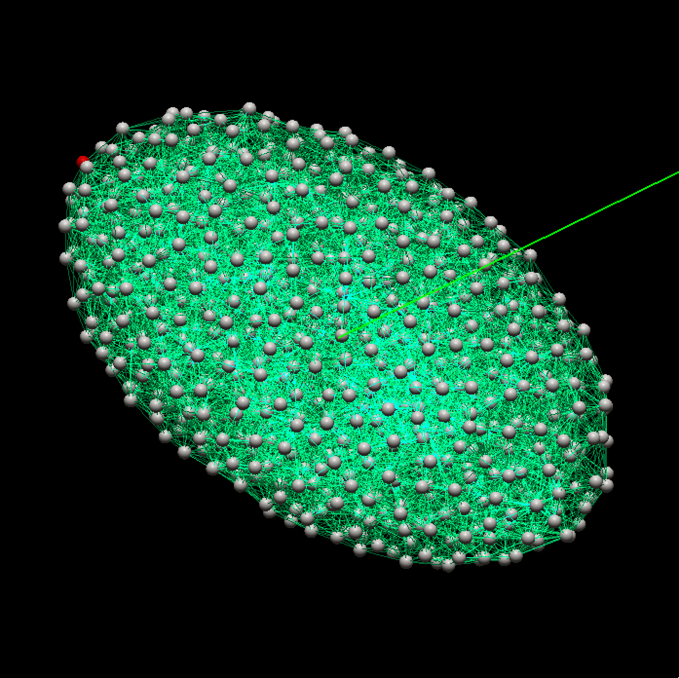
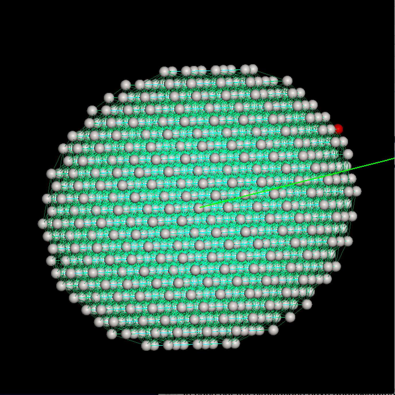
Figure 1: Two simulation snapshots. The top one shows a triaxial body from the random mass-spring model R series with $b/a=0.6$ and $c/a=0.5$ as seen looking down on the orbital plane. The bottom snapshot shows a cubic lattice simulation for an oblate body with $b/a=1.0$ and $c/a=0.7$. This simulation is seen from an inclined angle. The long green lines point to the tidally perturbing mass. A single mass node is colored red so that body libration can be viewed during tidal lock. The mass nodes are rendered as spheres with radius equal to 1/4 the minimum interparticle distance $d_{I}$ and spring connections are shown as thin green lines. The mass nodes are kept in their positions by spring elastic forces between nodes, not because the spherical surfaces repel.

2.1 Numerical comparisons and tests

The orbital parameters and mass ratio for our simulations are similar to those used by Frouard et al. (2016). In that paper we measured the sensitivity of the predicted to measured orbital semi-major axis drift rate to the size of the initial orbital semi-major axis. The ratio was independent of orbital semi-major axis, implying that for our adopted semi-major axis of 10 the torque is independent of the higher order terms in the expansion of the tidal gravitational potential.

For the spherical random R series simulations, we ran a comparison simulation using the adaptive time step 15th-order IAS15 integrator (Rein & Spiegel, 2015). The difference between measured drift rates was less than 0.02% implying that rebound’s faster and less accurate second order leap-frog integrator for our chosen step-size is sufficient for our study.

Gravitational interactions are still computed using the computationally intensive but accurate all particle pairs direct gravity routine in rebound as initial tests with the faster but less accurate tree-code were not promising. (A soft body that was barely strong enough to withstand self-gravity using the direct gravity computation imploded with the tree-code). Even at the semi-major axis of 10 and mass ratio of 10 (see Tables 1 and 2) the deformations are small and the orbital semi-major axis drift rates, listed for the spheres in Table 2, are of order $\dot{a}_{s}\sim 10^{-6}$. The gravity computation must be done accurately to measure tidal deformation and evolution. We leave development of tree or multipole gravity acceleration methods for future work.

Each time we run a simulation with a random spring network, a new set of particles is generated and this means there are variations in the spring network between simulations. To estimate the variation in measured semi-major axis drift rates due to differences in the spring network we ran 3 simulations with identical parameters, each in the R series of simulations, for the spherical body and for an oblate body with $c/a=0.5$ and for a prolate body with $c/a=0.5$. The standard deviation of $da_{o}/dt$ computed from each set of three simulations was less than 3% and smaller than the differences between the drift rates for simulations with body shapes that differ in axis ratios by 0.1. The R series of random lattice simulations has sufficient numbers of particles that differences in the generated spring networks only cause small variations in orbital semi-major axis drift rate.

In the random spring model, as particles are never generated outside the ellipsoid surface, there is a higher probability of generating particles just within the surface than near planar surfaces embedded within the body. This means that the surface is slightly denser than the interior. As springs are generated for each pair of particles within $d_{s}$, the strength of a region depends on the local particle density. Because there are more particles per unit volume near the surface, the surface is stronger than expected taking into account only the reduced number of springs per node due to the absence of particles outside the ellipsoid. A way around this problem is to generate a random distribution of particles in the same manor but in a larger region that contains our desired ellipsoid and then remove particles that lie outside the ellipsoid. We refer to models generated this way as soft-edged random spring models and those generated with our original procedure as hard-edged random spring models.

The hard and soft-edged types of random spring model simulations use the same set of parameters and only differ in their particle distribution. The soft-edged distribution is more uniform but the surface is more porous and weaker. Because there are fewer particles near the surface boundary the density gradient is shallower near the surface than for the hard-edged distribution (that is shown in Figure 1). The softer surface increases the drift rate, whereas the softer density profile would decrease it. We find that the soft-edged bodies have higher orbital semi-major axis drift rates so the softer edge is a more important factor affecting the tidal drift rate. For spherical bodies, the difference in drift rate (using the R series of parameters and between hard- and soft-edged bodies) is 20%, however the difference (between hard and soft) in drift rate for the prolate with $c/a=0.5$ is 43%. The difference depends on the body surface area and so the prolate models are more affected by the softer edge. Because the hard edge somewhat reduces the effect of the soft surface layer and how it affects the drift rates, we opted to run the random spring model simulations using our original method (hard-edged) for generating the random lattice particle distribution.

Even though the maximum spring length is smaller for the cubic lattice simulations (and so the thickness of the soft region reduced), because the number of springs per node is lower than for the random spring lattice, the surface layer for the cubic lattice can be quite weak. We could strengthen the surface layer by increasing the maximum spring length (so that there are more springs per node) but this has the effect of increasing the depth that is weaker than the interior and any advantage of using the cubic lattice model.

We also ran a series of random lattice model simulations with larger numbers of particles than the R series that we call the LR series. The LR series has about 2.5 times the number of mass nodes as the R series and takes about 6 times longer to run as gravity computations are done using all pairs of mass nodes (direct rather than using a tree code or a multipole algorithm). In the LR series we ran a spherical model, and oblate and prolate models with axis ratio $c/a=0.5$. We also ran a triaxial model with $b/a=0.8$ and $c/a=0.5$. When normalized to the drift rate of the spherical simulation in the same series we measured a difference between the ratio $\dot{a}_{o}/\dot{a}_{s}$ computed with 1200 particles (R series) and those computed with 3000 particles (LR series) that is less than 4% (when divided by the ratio computed with 3000 particles). There was no trend; the LR series ratios did not increase or decrease with axis ratio. This test suggests that we are running sufficient numbers of particles to ensure that the measured drift rates are not strongly sensitive to the structure of the surface spring network. However we must keep in mind that the R and LR series only differ by 2.5 in the number of particles and the maximum spring length (serving as a skin depth) is a significant faction of the volumetric radius in both cases ($d_{s}=0.33$ for the R series and 0.24 for the LR series).

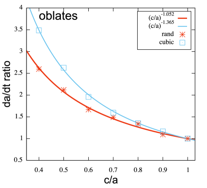
Figure 2: We show the drift rates in orbital semi-major axis due to tidal torque as a function of $c/a$ body axis ratio for simulated homogeneous viscoelastic oblate bodies ($a=b$) spinning about a minor axis with spin axis aligned with the orbital rotation axis. Measurements from two sets of simulations are shown as points, one based on a cubic lattice, the other using the random mass/spring model (C and R series with parameters listed in Table 2). The simulations in each series have approximately the same numbers of particles, springs per node, body volume and mass, shear modulus, viscoelastic relaxation timescale, initial spin, semi-major axis and perturber mass ratio. The differences are in the axis ratio of the simulated oblate ellipsoid. The vertical axis is $\dot{a}/\dot{a}_{s}$ where $\dot{a}_{s}$ is that measured for the spherical body in the simulation series. The horizontal axis shows body axis ratio $c/a$. The curves are power laws with best fitting index listed in the key.

3 Drift Rates Measured for Oblate Bodies

Bodies with $a=b$ and $a>c$ are oblate and here they are spinning about their short axis. Figure 2 plots as points drift rates measured for the oblate bodies from our simulations, normalized to the sphere with the same volume for the random R series and cubic C series simulations with parameters listed in Tables 1 and 2. With the points we have drawn power law curves $\dot{a}_{o}/\dot{a}_{s}=(c/a)^{-\alpha_{o}}$ with index $\alpha_{o}$ that gives the best fit to the numerically measured points. The index was measured using a nonlinear least-squares Marquardt-Levenberg algorithm and its standard deviation based on the rms value of the deviation of the simulation measurements from the fitted function. For the cubic lattice the best fit has $\alpha_{o}=1.365\pm 0.008$ whereas that for the random lattice simulations has $\alpha_{o}=1.052\pm 0.015$.

For an oblate body with spin parallel to the orbital axis and aligned with the body’s axis of symmetry, the shape of the tidally deformed body is independent of time. This suggests that we should consider how the drift rate depends on the equatorial radius, $R_{e}=a$. For the oblate ellipsoid, the volumetric radius

$$R_{v}=a(c/a)^{\frac{1}{3}}=R_{e}(c/a)^{\frac{1}{3}}.$$ (7)

We consider the hypothesis that equation 5 is appropriate for our oblate body but substituting the equatorial radius for the volumetric radius. Equation 5 gives $\dot{a}_{o}/(na_{o})$ as a unitless parameter so that it is independent of time, and we need not correct for the dependence of our unit of time on body radius (equation 1). The shear modulus, viscosity and viscoelastic relaxation timescales are the same for each simulation as are the body spin rate $\sigma$, semi-diurnal frequency $\omega$ and semi-diurnal frequency normalized with the viscoelastic relaxation time $\bar{\chi}$. Equation 5 shows that the orbital drift depends on radius to the 5-th power times the quality function. However equations 2 and 6 imply that when $\bar{\chi}<1$ the quality function is inversely proportional to radius to the 4-th power, due to the normalization of the elastic modulus (with $e_{g}\propto R_{v}^{-4}$). Taking into account the dependence of $e_{g}$ on radius $R$ we expect $\dot{a}_{o}/(na_{o})\propto R$. This implies that the ratio of the drift rate predicted using a classical tidal formula and replacing radius with equatorial radius when normalized with that using the volumetric radius is $\dot{a}_{o}/\dot{a}_{s}=(c/a)^{-1/3}$ as $R_{v}/a=(c/a)^{1/3}$. Our numerical measurements are not consistent with this scaling as we measured a power-law index 3 to 4 times larger in magnitude than 1/3.

4 Scaling estimates for the tidal drift rates of homogeneous triaxial ellipsoids

To better understand how the tidal torque and associated drift rate in semi-major axis depends on body axis ratio we estimate the torque on a tidally deformed triaxial body. The quadrupole moment of a mass distribution in Cartesian coordinates

$$Q_{ij}=\int\rho(3x_{i}x_{j}-\delta_{ij}r^{2})d^{3}x$$ (8)

where $\rho$ is the mass density. For a uniform triaxial ellipsoid with semi-axes $a,b,c$ and in coordinates aligned with body axes

$${\bf Q}=\frac{M}{5}\left(\begin{array}[]{ccc}2a^{2}-b^{2}-c^{2}&0&\\ 0&2b^{2}-a^{2}-c^{2}&0\\ 0&0&2c^{2}-b^{2}-a^{2}\end{array}\right)$$ (9)

with mass $M=\frac{4\pi}{3}\rho abc$. $Q$ is a tensor so we can rotate it; $Q^{\prime}=R(\theta)QR(\theta)^{-1}$ with $R(\theta)$ a rotation matrix. After rotation of the body by angle $\theta$ in the $xy$ plane we transform $Q$ to $Q^{\prime}$ finding off diagonal term

$$Q^{\prime}_{xy}=\frac{3}{10}M\sin(2\theta)(a^{2}-b^{2}).$$ (10)

Distant from the object the quadrupolar contribution to the gravitational potential

$$V_{2}({\bf x})=G\frac{Q_{ij}}{2}\frac{x_{i}x_{j}}{r^{5}}.$$ (11)

If a mass $M_{*}$ is located at $x=a_{o}$, $y=z=0$ then the $z$ component of the torque on it due to the quadrupolar force is

$$T = \left.M_{*}x\frac{\partial V_{2}}{\partial y}\right|_{x=a_{o},y=0,z=0}=\frac{GM_{*}Q^{\prime}_{xy}}{a_{o}^{3}}$$ (12)

$$= \frac{GMM_{*}}{a_{o}^{3}}\frac{3}{10}\sin(2\theta)(a^{2}-b^{2}).$$

This is equivalent to an application of MacCullagh’s formula for the instantaneous torque exerted by a planet on the permanent figure of an extended satellite. If $M_{*}$ causes tidal deformation of $M$ and $\theta$ is a lag angle (due to viscoelastic response) then this formula can be used to estimate the torque and associated spin down rate and semi-major axis drift rate (e.g., see Murray & Dermott 1999).

A three dimensional version of Hooke’s law relating stress applied on three Cartesian coordinates, $\sigma_{x},\sigma_{y},\sigma_{z}$ to strain in the three directions

$$\epsilon_{x} = \frac{1}{E}\left[\sigma_{x}-\nu(\sigma_{y}+\sigma_{z})\right]$$

$$\epsilon_{y} = \frac{1}{E}\left[\sigma_{y}-\nu(\sigma_{z}+\sigma_{x})\right]$$

$$\epsilon_{z} = \frac{1}{E}\left[\sigma_{z}-\nu(\sigma_{x}+\sigma_{y})\right]$$ (13)

where $\nu$ is the Poisson ratio and $E$ the Young’s modulus. More generally a linear relation between stress and strain or Hooke’s law in tensor form is $\sigma_{ij}=\lambda({\rm tr}\epsilon)\delta_{ij}+\mu\epsilon_{ij}$ with Lamé constants $\lambda,\mu$. In a coordinate system that diagonalizes the stress and strain tensors, Hooke’s law reduces to equations 13 as off-diagonal terms are zero.

The tidal acceleration on $M$ from distant mass $M_{*}$ with $M_{*}$ located at $x=a_{o}$, $y=z=0$ is

$${\bf a}_{T}\approx\frac{GM_{*}}{a_{o}^{3}}(2x,-y,-z)$$ (14)

taking only the quadrupolar term.

Instead of applying tidal force throughout the body (Dobrovolskis, 1982), we roughly approximate it as an instantaneously applied stress on the body surface.

We approximate the three stresses as scaling with the tidal acceleration, ${\bf a}_{T}$, on the surface, times mass, $M$, divided by cross sectional area (from the midplane perpendicular to the direction applied);

$$\sigma_{x} \sim \frac{GM_{*}M}{a_{o}^{3}}\frac{2a}{bc}$$

$$\sigma_{y} \sim -\frac{GM_{*}M}{a_{o}^{3}}\frac{b}{ac}$$

$$\sigma_{z} \sim -\frac{GM_{*}M}{a_{o}^{3}}\frac{c}{ab},$$ (15)

where we orient the body with semi-major axis $a$ along the $x$ axis, $b$ along the $y$ axis and $c$ along the z axis. Using Hooke’s law (in the form in equations 13) this gives surface strains of order

$$\epsilon_{x} \sim \frac{GM_{*}M}{a_{o}^{3}}\frac{1}{Eabc}(2a^{2}+\nu(b^{2}+c^{2}))$$

$$\epsilon_{y} \sim \frac{GM_{*}M}{a_{o}^{3}}\frac{1}{Eabc}(-b^{2}+\nu(c^{2}-2a^{2}))$$

$$\epsilon_{z} \sim \frac{GM_{*}M}{a_{o}^{3}}\frac{1}{Eabc}(-c^{2}+\nu(b^{2}-2a^{2})).$$ (16)

4.1 Scaling for Oblate bodies

An oblate body with unperturbed semi-major axes has $a=b$ and volumetric radius $R_{v}=a(c/a)^{1/3}$. Due to the tidal force the body becomes elongated in the equatorial plane with new semi-major and minor axes $a^{\prime}\approx a(1+\epsilon_{x})$ and $b^{\prime}\approx a(1+\epsilon_{y})$. We note that the moment $Q^{\prime}_{xy}$ depends on $a^{\prime 2}-b^{\prime 2}\mathrel{\vbox{ \offinterlineskip\halign{\hfil$#$\cr\propto\cr\kern 2.0pt\cr\sim\cr\kern-2.0pt\cr}}}\epsilon_{x}-\epsilon_{y}$. Inserting $a^{\prime},b^{\prime}$ into the formula for the torque (replacing $a^{\prime},b^{\prime}$ for $a,b$ in equation 12) and using equations 16 for the strains, we find that

$$T_{o}\mathrel{\vbox{ \offinterlineskip\halign{\hfil$#$\cr\propto\cr\kern 2.0pt\cr\sim\cr\kern-2.0pt\cr}}}\left(\frac{GMM_{*}}{a_{o}^{3}}\right)^{2}\frac{1}{Ea^{2}c}a^{4}(1+\nu).$$ (17)

We neglect variations in the lag angle $\theta$. Using the torque to estimate the semi-major axis drift rate (see equation 5)

$$\frac{\dot{a}_{o}}{na_{o}} \mathrel{\vbox{ \offinterlineskip\halign{\hfil$#$\cr\propto\cr\kern 2.0pt\cr\sim\cr\kern-2.0pt\cr}}} \left(\frac{M_{*}}{M}\right)\left(\frac{GM^{2}}{Ea^{4}}\right)\left(\frac{a}{a_{o}}\right)^{5}\frac{a}{c}$$ (20)

$$= \left(\frac{M_{*}}{M}\right)\left(\frac{GM^{2}}{ER_{v}^{4}}\right)\left(\frac{R_{v}}{a_{o}}\right)^{5}\left(\frac{c}{a}\right)^{-\frac{4}{3}}$$ (21)

where on the first line we are using the equatorial radius $a$ and on the second line the volumetric radius $R_{v}$ is used for scaling. The first line suggests that using the equatorial radius alone in the classic tidal formulae for spherical bodies would lead to an underestimate of the drift rate by the factor $a/c$. The dependence on $c$ arises because the estimated stresses (equations 15) and strains $\epsilon_{x},\epsilon_{y}$ (equations 16) depend on the inverse of the cross-sectional area. More physically, the strains in $x,y$, are dependent on the stress in the $z$ direction.

This series of approximations suggests that the drift rate for oblate bodies should scale with the axis ratio $c/a$ to the -4/3 power when normalized to a sphere with equivalent volume

$$\left(\frac{\dot{a}_{o}}{\dot{a}_{s}}\right)_{oblate}\approx\left(\frac{c}{a}\right)^{-\frac{4}{3}}.$$ (22)

This approximation is valid when the viscoelastic relaxation time times the tidal frequency $\bar{\chi}<1$. If the tidal frequency is large compared to the inverse of the viscoelastic relaxation timescale then the scaling would be different as then the quality function is not proportional to shear modulus normalized to $e_{g}$.

4.2 Comparison of scaling for oblate bodies with the measurements from simulations

The index -4/3 from equation 22 is closer to the index $-1.05$ that we measured for the random lattice model (see section 3 and Figure 2) than the -1/3 estimated using the equatorial radius alone in the classical tidal formula. The stronger dependence on $c$ arises because the stresses and strains depend on the body cross sectional area.

The body surface area is larger for more extreme axis ratio ellipsoids than the equivalent sphere. The soft surface layer present in the simulations should increase the drift rates compared to what is expected in the continuum limit. We can consider our numerically measured points to be an upper limit for the value approached with larger numbers of simulated particles as we expect that numerically generated surface softness increases the drift rates. However we must keep in mind that our hard-edged bodies (see discussion in section 2.1) also have slightly higher density near the surface than a homogeneous body and we are not sure how this would have affected the numerical measurements, though we suspect that the weak surface has a stronger influence on the drift rates. As our numerical measurements are likely to be upper limits, we suspect that a more rigorous calculation (better than in section 4.1) would predict a reduced exponent (flatter than 4/3).

The cubic lattice simulations have best fitting index $-1.365$ and this is closer to the -4/3 power predicted by equation 22. However, as we discuss below, our measurements for oblate and triaxial bodies imply that the cubic lattice simulations badly approximate elastically isotropic bodies.

4.3 Scaling for Triaxial bodies

Orienting the long axis of a triaxial body along the $x$ axis (setting the tide) and using equation 16 gives us strain values for a tidally deformed triaxial body. The aligned but tidally deformed body has semi-major axis $a^{\prime}=a(1+\epsilon_{x})$ and $b^{\prime}=b(1+\epsilon_{y})$ giving torque (inserting $a^{\prime}$ and $b^{\prime}$ for $a,b$ into equation 12)

$$T_{a}\mathrel{\vbox{ \offinterlineskip\halign{\hfil$#$\cr\propto\cr\kern 2.0pt\cr\sim\cr\kern-2.0pt\cr}}}a^{2}-b^{2}+2a^{2}\epsilon_{x}-2b^{2}\epsilon_{y}$$ (23)

and we have neglected terms dependent on the Poisson ratio. The term independent of the strain should average to zero (and we will see that makes sense below when we estimate the torque for the same body but rotated by $90^{\circ}$ with respect to $M_{*}$). We compute

$$a^{2}\epsilon_{x}-b^{2}\epsilon_{y}\sim\frac{GMM_{*}}{a_{o}^{3}}\frac{1}{Eabc}(2a^{4}+b^{4}).$$ (24)

We now consider the same body but rotated by $90^{\circ}$ (as it can be if rotating about the $z$ axis). If the middle axis of the body $b$ is oriented along the $x$ axis then

$$\sigma_{x} \sim \frac{GM_{*}M}{a_{o}^{3}}\frac{2b}{ac}$$

$$\sigma_{y} \sim -\frac{GM_{*}M}{a_{o}^{3}}\frac{a}{bc}$$

$$\sigma_{z} \sim -\frac{GM_{*}M}{a_{o}^{3}}\frac{c}{ab}$$ (25)

(recall $x$ is along the tidal axis) giving strains

$$\epsilon_{x} \sim \frac{GM_{*}M}{a_{o}^{3}}\frac{1}{Eabc}(2b^{2}+\nu(a^{2}+c^{2}))$$

$$\epsilon_{y} \sim \frac{GM_{*}M}{a_{o}^{3}}\frac{1}{Eabc}(-a^{2}+\nu(c^{2}-2b^{2}))$$

$$\epsilon_{z} \sim \frac{GM_{*}M}{a_{o}^{3}}\frac{1}{Eabc}(-c^{2}+\nu(a^{2}-2b^{2})).$$ (26)

For the prolate body oriented with $b$ axis along $x$ we have deformed axes $a^{\prime}=b(1+\epsilon_{x})$, $b^{\prime}=a(1+\epsilon_{y})$ and the resulting torque (replacing $a^{\prime},b^{\prime}$ for $a,b$ in equation 12) is

$$T_{b}\mathrel{\vbox{ \offinterlineskip\halign{\hfil$#$\cr\propto\cr\kern 2.0pt\cr\sim\cr\kern-2.0pt\cr}}}b^{2}-a^{2}+2b^{2}\epsilon_{x}-2a^{2}\epsilon_{y}.$$ (27)

We compute

$$b^{2}\epsilon_{x}-a^{2}\epsilon_{y}\sim\frac{GMM_{*}}{a_{o}^{3}}\frac{1}{Eabc}(2b^{4}+a^{4}).$$ (28)

Taking an average of the two torques $T_{a}$ and $T_{b}$ we see that the terms independent of strain cancel. The torque averaged over rotation (and neglecting angular dependence of phase angle $\theta$), is approximated from the average of the two orientations,

$$T\mathrel{\vbox{ \offinterlineskip\halign{\hfil$#$\cr\propto\cr\kern 2.0pt\cr\sim\cr\kern-2.0pt\cr}}}\frac{GMM_{*}}{a_{o}^{3}}\frac{GM_{*}M}{a_{o}^{3}}\frac{1}{Eabc}(a^{4}+b^{4}).$$ (29)

The associated drift rate for a triaxial body we estimate as

$$\frac{\dot{a}_{o}}{na_{o}} \mathrel{\vbox{ \offinterlineskip\halign{\hfil$#$\cr\propto\cr\kern 2.0pt\cr\sim\cr\kern-2.0pt\cr}}} \left(\frac{M_{*}}{M}\right)\left(\frac{GM^{2}}{Ea^{4}}\right)\left(\frac{a}{a_{o}}\right)^{5}$$ (34)

$$\times\left(1+\frac{b^{4}}{a^{4}}\right)\left(\frac{b}{a}\right)^{-1}\left(\frac{c}{a}\right)^{-1}$$

$$= \left(\frac{M_{*}}{M}\right)\left(\frac{GM^{2}}{ER_{v}^{4}}\right)\left(\frac{R_{v}}{a_{o}}\right)^{5}$$

$$\times\left(1+\frac{b^{4}}{a^{4}}\right)\left(\frac{b}{a}\right)^{-\frac{4}{3}}\left(\frac{c}{a}\right)^{-\frac{4}{3}}.$$

When normalized to the drift rate for an equivalent volume sphere, the triaxial bodies should have drift rates

$$\left(\frac{\dot{a}_{o}}{\dot{a}_{s}}\right)_{triaxial}\approx\frac{1}{2}\left(1+\frac{b^{4}}{a^{4}}\right)\left(\frac{b}{a}\right)^{-\frac{4}{3}}\left(\frac{c}{a}\right)^{-\frac{4}{3}},$$ (35)

where the factor of 1/2 is so that when $a=b=c$ the ratio is 1. The dependence on $1+\frac{b^{4}}{a^{4}}$ arises from averaging over body rotation whereas the dependence on $(b/a)^{-\frac{4}{3}}(c/a)^{-\frac{4}{3}}$ is from the dependence of tidal stress on cross sectional area.

These order of magnitude scaling estimates do not compute the stress and strain fields accurately, take into account rotational deformation nor do they appropriately average over body rotation.

5 Measurements of Drift Rates for Prolate and Triaxial Bodies

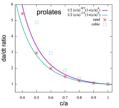
Figure 3: We show drift rates in orbital semi-major axis as a function of body axis ratio $c/a$ for simulated viscoelastic prolate bodies (with $b=c$) spinning about minor axis and with spin axis aligned with the orbital axis. Measurements from two sets of simulations are shown as points, one based on a cubic lattice (the C series), the other using the random mass/spring model (the R series). The simulations in each series have approximately the same numbers of particles, springs per node, body volume and mass, shear modulus, viscoelastic relaxation timescale, initial spin, semi-major axis and perturber mass ratio. The differences are in the axis ratio of the simulated prolate ellipsoid. The vertical axis is $\dot{a}/\dot{a}_{s}$ where $\dot{a}_{s}$ is that measured for the spherical body in the simulation series. The horizontal axis shows body axis ratio $c/a=b/a$. The drift rates are poorly fit by a power law. Shown as two curves are equations 36 and 37. Equation 36 is based on order of magnitude stress/strain estimates in section 4.3. These relations are good matches to the random spring model simulations.

5.1 Prolate Bodies

For the prolate systems, the long axis of the body rotates in the orbital plane and $b=c$. Figure 3 is similar to Figure 2 but here we only plot the prolate bodies. Power law functions of any index give poor fits to either cubic or random lattice prolate simulations.

For a prolate system with $b=c$ our scaling estimate in equation 35 implies that

$$\left(\frac{\dot{a}_{o}}{a_{s}}\right)_{prolate}\sim\frac{1}{2}\left(1+\frac{c^{4}}{a^{4}}\right)\left(\frac{c}{a}\right)^{-\frac{8}{3}}.$$ (36)

However if we take into account that we measured a power law dependence of -1.05 for the oblate systems then we might expect

$$\left(\frac{\dot{a}_{o}}{a_{s}}\right)_{prolate}\sim\frac{1}{2}\left(1+\frac{c^{4}}{a^{4}}\right)\left(\frac{c}{a}\right)^{-2.4}$$ (37)

as $4/3+1.05\approx 2.4$. We plot both of these curves on Figure 3, finding that both functions are adequate matches to the prolates from the random spring model simulations but not the cubic lattice ones. Fitting the curve $\frac{1}{2}\left(1+\frac{c^{4}}{a^{4}}\right)\left(\frac{c}{a}\right)^{-\alpha_{p}}$ we find a best fitting index of $\alpha_{p}=2.555\pm 0.017$ for the random spring model and $\alpha_{p}=3.367\pm 0.027$ for the cubic lattice spring model simulations.

At extreme axis ratios, the drift rates for the cubic lattice are much higher than those of the random lattice (when compared to their matching spherical body). The $c/a=0.4$ prolate body cubic lattice model drift rate has a ratio of $\dot{a}_{o}/\dot{a}_{s}=11.6$ and lies above the limits of the plot in Figure 3. This value is more than twice the value for the random-spring model prolate with $c/a=0.4$. The best fitting index for the random spring models $\alpha_{p}=2.56$ is near that predicted from scaling estimates, $8/3\approx 2.67$. However the best fitting index for the cubic lattice model, $3.37$, is much higher than expected.

In section 4.3 we estimated the drift rate by averaging the torque with body orientation along the tidal axis and that oriented perpendicular to the tidal axis. While the strain for the cubic lattice in $x$ and $y$ directions (with respect to the orientation of a cubic cell in the lattice) is the same, the body is weaker when stresses are applied along a direction $45^{\circ}$ from an edge of the cubic cell and in a plane containing a cubic cell face. Consequently our averaging procedure underestimates the average tidal deformation. This is likely a stronger affect when the axis ratios are high even when normalizing to the matching sphere which is also affected by the elastic anisotropy of the cubic lattice. The cubic lattice has a shallower but softer surface (due to a lower number of springs per node) than the random spring model and this too might contribute to the stronger sensitivity of the drift rate to axis ratio compared to the random spring model. We can attribute the high drift rates at low axis ratios for both oblate and prolate bodies (and a stronger affect for the prolates) to the anisotropy of the lattice.

The strong dependence of drift rates on axis ratios emphasizes that the drift rates are strongly influenced by the weakest part of the simulated body. When prolate, the body is easiest to deform along its long axis, when a cubic lattice is present, the drift rate is strongly influenced by the elastic anisotropy. Softness in the simulated body surface is likely our largest source of error in estimating tidally induced drift rates with the random lattice models. A real asteroid or Kuiper belt object if it contains soft materials, discontinuities or fractures, may be poorly approximated by a homogeneous strength viscoelastic model.

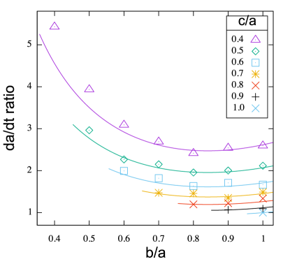
Figure 4: Orbital semi-major axis drift rates for triaxial bodies measured from the random spring model simulations from the R series. The vertical axis is $(\dot{a}/\dot{a}_{s})$ where $\dot{a}_{s}$ is that measured for the spherical body. The horizontal axis shows $b/a$ body axis ratio. Bodies with different values of $c/a$ have different point types. The key on the upper right shows the body axis ratio $c/a$ for each point type. Oblate bodies lie on the far right. The curves show equation 38, each line with a different value of $c/a$ and with line color matching the numerically measured points with the same value.

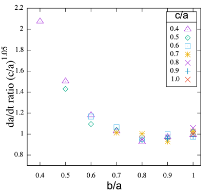
Figure 5: We show the orbital semi-major axis drift rates measured from the R series of random spring model simulations but corrected by $(c/a)^{1.05}$ with power index based on the power law that fit the oblate simulations. The vertical axis is $\dot{a}/\dot{a}_{s}\times(c/a)^{1.05}$ where $\dot{a}_{s}$ is that measured for the spherical body. Once corrected for the axis ratio $c/a$, the drift rates for the triaxial bodies resemble those of the prolate bodies.

5.2 Triaxial bodies

Figure 4 shows (as points) the numerically measured normalized drift rates for the R series of random spring models and for triaxial bodies with $c/a=1.0,0.9,0.8,0.7,0.5,0.4$ and $b/a$ covering the same range but with $b/a\geq c/a$ so they are stable as the bodies are rotating about the short axis. On this figure the point type labels $c/a$ and the drift rates are plotted versus $b/a$. The oblate bodies lie on the right hand side of the plot and the prolate bodies lie to the left of the diagonal connecting upper left to lower right. Taking the power law approximations for the oblate bodies we correct the drift rates by $(c/a)^{1.05}$ and replot the points in Figure 5. In Figure 5 we see that the points lie on a curve that is similar to that of the prolate bodies (see Figure 3). This implies that the drift rate can be considered to be a product of two functions; one that depends on $c/a$ and is approximately a power law, and the other that depends on $b/a$.

Our scaling estimate presented in section 4.3 suggested that the drift rate should be a product with form in equation 35. That correcting for $c/a$ puts the triaxial drift rates on the same line as the oblates supports the expectation (based on the order of magnitude estimates) that the drift rates can be approximated by a product of functions, one depending on $c/a$ and the other on $b/a$.

The oblate random lattice models were better fit with a function proportional to $(c/a)^{-1.05}$ rather than $(c/a)^{-4/3}$, so in Figure 4 we have plotted on top of the numerically measured points curves generated with

$$\left(\frac{\dot{a}_{o}}{\dot{a}_{s}}\right)_{triaxial}\approx\frac{1}{2}\left(1+\frac{b^{4}}{a^{4}}\right)\left(\frac{b}{a}\right)^{-\frac{4}{3}}\left(\frac{c}{a}\right)^{-1.05}.$$ (38)

This function is a pretty good match to all the simulations shown in Figure 4. The slight increase at $b/a$ near 1 is reproduced by both simulations and the estimating scaling behavior. Had we plotted curves using equation 35, the curves would have matched the prolate points on the left but would have diverged from the oblate plots on the right hand side of the plot. We conclude that the random spring models are probably accurate and that the function estimated in the section, equation 35, is a good approximation, though the power-law index for $c/a$ may be somewhat shallower than -4/3, as given in equation 38.

6 Discussion on Haumea

Table 3: Information about Haumea and Hi’iaka

Haumea:
Semi-major axis of ellipsoid	$a_{H}$	960 km
Axis ratio	$b_{H}/a_{H}$	0.80
Axis ratio	$c_{H}/a_{H}$	0.52
Volumetric radius	$R_{vH}$	716.6 km
Mass of Haumea	$m_{H}$	$4\times 10^{21}$ kg
Energy density scale	$e_{g,H}$	4.05 GPa
Gravitational timescale	$t_{g}$	1171 s
Spin rate	$\sigma_{H}t_{g}$	0.52
Tidal frequency	$\omega\sim 2\sigma_{H}$	$0.9\times 10^{-3}$ Hz
Mass ratio	$q=M_{Hi}/M_{H}$	0.0045
orbital semi-major axis Hi’iaka	$a_{Hi}$	49880 km

Body semi-major axis and axis ratios are by Lockwood et al. (2014). Mass of Haumea, mass ratio, $q$, of Hi’iaka and Haumea and semi-major axis are by Ragozzine & Brown (2009). The volumetric radius $R_{vH}$ is the radius of a sphere with the same volume as the triaxial ellipsoid. Spin rate, gravitational timescale, $t_{g}$ and energy density scale, $e_{g}$, are computed using the volumetric radius and equations 1 and 2. The spin rate was computed using the spin period $P_{H}=2\pi/\sigma_{H}=3.91531\pm 0.00005$ hours measured by Lockwood et al. (2014).

The dwarf planet Haumea (Brown et al., 2005) is an extremely fast rotator with density higher than other objects in the Kuiper belt; it is consistent with a body dominated by rock (Rabinowitz et al., 2006; Lacerda et al., 2008; Lellouch et al., 2010; Kondratyev, 2016). Visible and infrared light curve fits (Lockwood et al., 2014) find the body consistent with a rapidly rotating oblong Jacobi ellipsoid shape in hydrostatic equilibrium with axis ratios listed in Table 3 (also see Lellouch et al. 2010) and a density of $\rho=2.6$ g cm^-3. For discussion on formation scenarios for the satellite system see Leinhardt et al. (2010); Schlichting & Sari (2009); Cuk et al. (2013). Parameters based on Haumea and Hi’iaka are listed in Table 3.

The pressures in the body at depth for a body as massive as Haumea would lead to ductile flow giving long-term deformation allowing the body to approach a figure of equilibrium (a Jacobi ellipsoid). Even if Haumea’s shape is consistent with a hydrostatic equilibrium figure, on short timescales the body should behave elastically. For tidal evolution, the relevant tidal frequency is $\omega\sim 2\sigma_{H}\sim 10^{-3}$Hz, comparable to vibrational normal mode frequencies in the Earth. Our simulations do not allow ductile flow on long timescales, but can approximate the faster tidal deformations if we model the body as a stiff elastic body with its current shape.

We ran a simulation in the LR random lattice series with axis ratios $b/a=0.8$ and $c/a=0.5$, consistent with measurements for Haumea. The LR series of simulations has more particles than the R series and is discussed in more detail in section 2.1. From the simulation we measure $\dot{a}_{o}/a_{s}=2.04$ or drift rate approximately twice that of the equivalent volume sphere. Equation 38 predicts a value 2.034, consistent with the numerical measurement, whereas equation 35 gives 2.39. In their section 4.3.1, Ragozzine & Brown (2009) speculated that using the volumetric radius leads to an underestimate of the tidal evolution. However for the axis ratio of Haumea $b/a\approx 0.8$ and $c/a\approx 0.52$, we find here that the drift rate would only be about twice as fast as estimated using the volumetric radius.

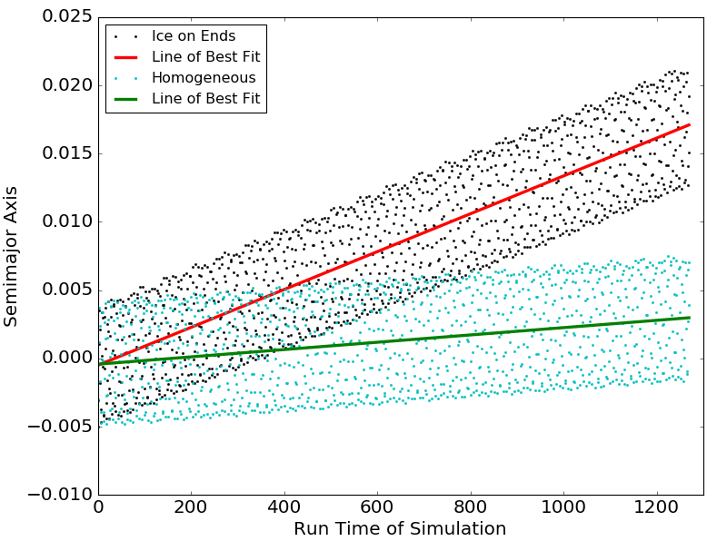
Figure 6: We compare the drift rate in orbital semi-major axis for two simulations in the LR series and with axis ratios $b/a=0.8$ and $c/a=0.6$, similar to Haumea. The blue points show a simulation of a homogeneous body, whereas the black points show a simulation with weaker ends (where springs have a lower spring constant), mimicking a rocky body with icy ends. The lines show linear fits measuring the secular drift rate. The $x$ axis shows time in units of $t_{g}$ (equation 1) and the $y$ axis shows semi-major axis in units of volumetric radius, $R_{v}$, measured from the initial value. The drift rate of the body with soft ends is about 5.2 times faster than the homogeneous ellipsoid with the same axis ratios and about 10 times faster than the equivalent volume homogeneous sphere.

Kondratyev (2016) proposed that stresses between icy shell and core and associated relaxation would cause ice to accumulate at the ends of Haumea. He proposed that the icy ends could separate forming the two icy satellites Namaka and Hi’iaka. Estimates for the fraction of ice in a differentiated Haumea range from 7% (Kondratyev, 2016) to 30% (Probst et al., 2015).

Young’s modulus of ice is estimated to be a few GPa (Nimmo & Schenk 2006; see Collins et al. 2010 for a review) and this is about 10 times lower than the Young’s modulus for rocky materials. To explore the affect of softer icy ends on the semi-major axis drift rate, we ran a simulation of a body that is not homogeneous. Using the same axis ratios of $b/a=0.8$ and $c/a=0.5$ and parameters of the LR series, we reduced the spring constants to 1/10th the value in the body core at radii greater than 1 (in units of volumetric radius) from the body center. About 20% of the springs have reduced spring constants. This has the effect of lowering the simulated Young’s modulus at the ends of the ellipsoid by a factor of 10. We did not vary the density as the difference in density between ice and rock is much lower than their difference in elastic modulus. The spring damping parameter $\gamma$ does not vary, so $\tau$, the viscoelastic relaxation time-scale, and tidal frequency, $\bar{\chi}$, are the same in both regions. The measurements of semi-major axis for this simulation and for the homogeneous one with the same axis ratios are shown in Figure 6 along with linear fits that measure the secular drift rate. We measured the drift rate in semi-major axis in this simulation, finding that it is about 5.2 times faster than the homogeneous ellipsoid with the same axis ratios and 10 times faster than the equivalent homogeneous sphere. Even a small fraction of softer material can significantly affect the simulated drift rates. Perhaps this should have been expected based on the strong sensitivity to elastic anisotropy that we inferred from the cubic lattice model simulations.

The classical tidal formula for the tidal drift rate in semi-major axis

$$\frac{\dot{a}_{o}}{na_{o}}=\frac{3k_{2H}}{Q_{H}}\frac{M_{*}}{M_{H}}\left(\frac{R_{vH}}{a_{o}}\right)^{5}$$ (39)

(e.g., Murray & Dermott 1999) for perturbing object $M_{*}$ (here Hi’iaka) due to tidal dissipation in the spinning body $M_{H}$, where $k_{H}$ and $Q_{H}$ are the Love number and dissipation factor for Haumea. We can describe corrections to the tidal drift rate by multiplying the right hand side by a parameter $f_{corr}>1$. The above equation implies that $\dot{a}_{o}\propto a_{o}^{-5.5}$ (taking into account dependence on $na_{o}\propto a_{o}^{-1/2}$). We integrate the above equation for Haumea to estimate the time it takes Hi’iaka to tidally drift outwards to its current semi-major axis. Putting unknowns on the left hand side

$$\frac{k_{2H}}{Q_{H}}f_{corr}\sim\frac{1}{n\tau_{a}}\left(\frac{a_{Hi}}{R_{v}}\right)^{5}\frac{2}{39}q^{-1}\sim 0.1$$ (40)

with mass axis ratio $q=M_{Hi}/M_{H}$ and where we have used values from Table 3 and an age $\tau_{a}=4$ Gyr for the timescale over which tidal migration is taking place. Here $n$ and $a_{Hi}$ are the mean motion and orbital semi-major axis of Hi’iaka at its current location. If $k_{2H}$ for Haumea is as large as 0.01 (at the border of what would be consistent with rigidity for rocky material) and we use corrections for shape and composition increasing the drift rate by $f_{corr}=10$ then we have equality only if the dissipation parameter is large; $Q\sim 1$. We conclude that it is unlikely that Hi’iaka alone tidally drifted to its current location even if the tidal drift rate is larger by a factor of 10 than estimated using the equivalent volume rocky sphere.

One explanation for the origin of Haumea’s satellites and compositional family is a collisional disruption of a past large moon of Haumea (Schlichting & Sari, 2009). The ‘ur-satellite’ would have formed closer to Haumea and because of its large mass, could have migrated more quickly than Hi’iaka outward during the lifetime of the Solar system. The failure of our enhanced tidal drift rate estimate to account for Hi’iaka’s current position would suport the ‘ur-satellite’ proposal (also see discussion by Cuk et al. 2013).

7 Summary and Discussion

Motivated by the discovery of spinning elongated bodies such as Haumea, we have carried out a series of mass-spring model simulations to measure the tidally induced drift rate (in orbital semi-major axis) of homogeneous spinning viscoelastic triaxial ellipsoids in a circular orbit about a point mass. We have restricted this initial study to bodies spinning about the shortest principal body axis aligned with the orbital axis and with tidal frequency times the viscoelastic timescale $\bar{\chi}\ll 1$, sufficiently small to ensure that the torque is linear in $\bar{\chi}$.

Our simulations and order of magnitude estimates show that the tidal torque or associated orbital semi-major axis drift rates, when normalized by that of a spherical body of equivalent volume, are described by

$$\frac{\dot{a}_{o}}{\dot{a}_{s}}\approx\frac{1}{2}\left(1+\frac{b^{4}}{a^{4}}\right)\left(\frac{b}{a}\right)^{-\frac{4}{3}}\left(\frac{c}{a}\right)^{-\alpha_{c}}$$ (41)

with $\alpha_{c}\approx 1.05$ consistent with our random lattice simulations but $\alpha_{c}=4/3$ predicted via order of magnitude estimates. This function is a good match to the prolate simulations using either value of $\alpha_{c}$ but better matches the oblate and all the triaxial ones with $\alpha_{c}\approx 1.05$.

For a homogeneous body with axis ratios equal to those of Haumea ($b/a\approx 0.8$, $c/a\approx 0.5$) we estimate that the drift rate in orbital semi-major axis is about twice as fast as that estimated for a spherical body with the same mass and volume. Motivated by the proposal that ice could have accumulated at Haumea’s ends (Kondratyev, 2016) we also ran a simulation of a non-homogeneous body with 20% of the springs (those at the ends of the body) set at 1/10th the strength of those in the core, approximating a body comprised of two materials, ice and rock. This simulation has a drift rate 10 times higher than the equivalent homogeneous sphere. Reexamining the tidal evolution of Hi’iaka, we find that even this increase by 10 is insufficient to have allowed Hi’iaka to have drifted tidally to its current location via tidal interaction with Haumea alone. We have only considered the behavior of a solid body with fixed axis ratios and a static viscoelastic rheology and we have neglected the role of Namaka. More complex models, perhaps taking into account how material properties and their distribution are affected by the tidally induced heat, could reexamine this conclusion.

We experimented with using a cubic lattice distribution for simulated mass nodes, but suspect that the random spring model is more accurate because it is elastically isotropic, even though the cubic lattice is more homogeneous and can be set up with shorter springs at the same number of mass nodes. The random spring model is hampered by a soft and weak surface region with depth set by the maximum length of the springs. Until we speed up the gravity computation (perhaps using a multipole method) we cannot on a single processor increase the number of particles past a few thousand so as to reduce the effect of the soft surface layer.

Spin orbit resonances and vibrational modes have been neglected from this study and the order of magnitude scaling estimates rely on crude approximation for the stresses associated with tidal acceleration. The mass spring model approximates a Kelvin-Voigt viscoelastic rheology with Poisson ratio of 1/4 rather than an incompressible Maxwell or Andrade rheology. Recently developed methods (e.g., Wisdom 2008; Mathis & Le Poncin-Lafitte 2009; Panou 2014) might be modified or extended to improve upon the scaling arguments presented here. Future work, both analytical and numerical, will be required to improve upon the accuracy of tidal computations for bodies with extreme axis ratios.

We are grateful to Valery Lainey, Dan Scheeres, Dan Tamayo and Michael Efroimsky for helpful discussions and correspondence. This work was improved with helpful and encouraging comments from the referee, Benoît Noyelles. This work was in part supported by the NASA grant NNX13AI27G and NSF award PHY-1460352.

References

- Breiter et al. (2012) Breiter, S., RoZek, A., & Vokrouhlicky, D. 2012, MNRAS, 427, 755-769, Stress field and spin axis relaxation for inelastic triaxial ellipsoids
- Brown et al. (2005) Brown, M.E., Bouchez, A.H., Rabinowitz, D.L., Sari, R., Trujillo, C.A., van Dam, M., Campbell, R., Chin, J., Hartman, S., Johansson, E., Lafon, R., LeMignant, D., Stomski, P., Summers, D., & Wizinowich, P., 2005, Astrophys. J. Lett. 632, L45 -L48. Keck Observatory Laser Guide Star Adaptive Optics Discovery and Characterization of a Satellite to the Large Kuiper Belt Object 2003 EL61.
- Collins et al. (2010) Collins, G. C., McKinnon, W. B., Moore, J. M., Nimmo, F., Pappalardo, R. T., Prockter L. M., & Schenk, P. M., 2010. Tectonics of the outer planet satellites. In: Watters, T. R., Richard A. Schultz, R. A. (Eds.), Planetary Tectonics, Cambridge University Press, Cambridge England, pp. 264-350.
- Cuk et al. (2013) Cuk, M., Ragozzine, D., & Nesvorny, D. 2013, Astronomical Journal, 146, 89-102. On the Dynamics and Origin of Haumea’s Moons
- Dobrovolskis (1982) Dobrovolskis, A R. 1982, Icarus, 52, 136-148. Internal Stresses in Phobos and other Triaxial bodies
- Efroimsky & Makarov (2013) Efroimsky, M., & Makarov, V. V. 2013. Astrophysical Journal, 764, 26. Tidal Friction and Tidal Lagging. Applicability Limitations of a Popular Formula for the Tidal Torque.
- Efroimsky & Lainey (2007) Efroimsky, M., & Lainey, V. 2007. Journal of Geophysical Research – Planets, 112, E12003. The Physics of Bodily Tides in Terrestrial Planets and the Appropriate Scales of Dynamical Evolution.
- Efroimsky & Williams (2009) Efroimsky, M., & Williams, J. G. 2009. Celestial Mechanics and Dynamical Astronomy, 104, 257 - 289. Tidal torques: a critical review of some techniques.
- Efroimsky (2015) Efroimsky, M. 2015. Astronomical Journal, 150, 98. Tidal Evolution of Asteroidal Binaries. Ruled by Viscosity. Ignorant of Rigidity.
- Ferraz-Mello et al. (2008) Ferraz-Mello, S., Rodríguez, A., & Hussmann, H. 2008. Celestial Mechanics and Dynamical Astronomy, 101, 171 - 201. Tidal friction in close-in satellites and exoplanets: The Darwin theory re-visited.
- Ferraz-Mello (2013) Ferraz-Mello, S. 2013, Celestial Mechanics and Dynamical Astronomy, 116, 109, Tidal synchronization of close-in satellites and exoplanets. A rheophysical approach.
- Frouard et al. (2016) Frouard, J., Quillen, A. C., Efroimsky, M., & Giannella, D. 2016, MNRAS, 458, 2890-2901, Numerical Simulation of Tidal Evolution of a Viscoelastic Body Modelled with a Mass-Spring Network.
- Goldreich (1963) Goldreich P. 1963, MNRAS, 126, 257-268. On the eccentricity of satellite orbits in the solar system.
- Goldreich & Peale (1968) Goldreich, P., & S. J. Peale, S. J. 1968. Ann. Rev. Astron. Astrophys., 6, 287-320. The dynamics of planetary rotations.
- Kaula (1964) Kaula, M. 1964. Reviews of Geophysics, 2, 661 - 684. Tidal Dissipation by Solid Friction and the Resulting Orbital Evolution.
- Kondratyev (2016) Kondratyev, B. P. 2016, Astrophys. Space Sci. 361, 169, The near-equilibrium figure of the dwarf planet Haumea and possible mechanism of origin of its satellites.
- Kot et al. (2015) Kot, M., Nagahashi, H., & Szymczak, P. 2015. “Elastic moduli of simple mass spring models”, The Visual Computer: International Journal of Computer Graphics, 31, 1339 - 1350.
- Lacerda et al. (2008) Lacerda, P., Jewitt, D., & Peixinho, N. 2008, Astronomical Journal, 135, 1749-1756, High-Precision Photometry of Extreme KBO 2003 EL61
- Leinhardt et al. (2010) Leinhardt, Z. M., Marcus, R. A., & Stewart, S. T. 2010, Astrophysical Journal, 714, 1789-1799, The Formation of the Collisional Family Around the Dwarf Planet Haumea.
- Lellouch et al. (2013) Lellouch, E., Santos-Sanz, P., Lacerda, P., Mommert, M., Duffard, R., Ortiz, J. L., Müller, T. G., Fornasier, S., Stansberry, J., Kiss, C., Vilenius, E., Mueller, M., Peixinho, N., Moreno, R., Groussin, O., Delsanti, A., & Harris, A. W. 2013, A&A, 557, A60
- Lellouch et al. (2010) Lellouch, E., Kiss, C., Santos-Sanz, P., Müller, T. G., Fornasier, S., Groussin, O., Lacerda, P., Ortiz, J. L., Thirouin, A., Delsanti, A., Duffard, R., Harris, A. W., Henry, F., Lim, T., Moreno, R., Mommert, M., Mueller, M., Protopapa, S., Stansberry, J., Trilling, D., Vilenius, E., Barucci, A., Crovisier, J., Doressoundiram, A., Dotto, E., Gutierrez, P. J., Hainaut, O., Hartogh, P., Hestroffer, D., Horner, J., Jorda, L., Kidger, M., Lara, L., Rengel, M., Swinyard, B., & Thomas, N. 2010, A&A, 518, L147+
- Lockwood et al. (2014) Lockwood, A. C., Brown, M. E., & Stansberry, J. 2014, Earth Moon & Planets, 111, 127-137, The Size and Shape of the Oblong Dwarf Planet Haumea.
- Love (1927) Love, A. 1927. “A Treatise on the Mathematical Theory of Elasticity.” Dover, New York.
- Mathis & Le Poncin-Lafitte (2009) Mathis, S. & Le Poncin-Lafitte C. 2009, Astronomy & Astrophysics , 497, 889-910. Tidal dynamics of extended bodies in planetary systems and multiple stars
- Murray & Dermott (1999) Murray, C. D. & Dermott, S. F. 1999. “Solar System Dynamics”. Cambridge University Press, Cambridge.
- Nimmo & Schenk (2006) Nimmo, F., & Schenk, P., 2006. J. Struct. Geol., 28, 2194-2203. Normal faulting on Europa: Implications of ice shell properties.
- Noyelles et al. (2014) Noyelles, B., Frouard, J., Makarov, V.V., & Efroimsky, M. 2014, Icarus, 241, 26-44. Spin-orbit evolution of Mercury revisited.
- Ogilvie (2014) Ogilvie, G. I. 2014, ARA&A, 52, 171, Tidal Dissipation in Stars and Giant Planets
- Panou (2014) Panou, G. 2014, Studia Geophysica et Geodaetica, 58, 609-625, The gravity field due to a homogeneous triaxial ellipsoid in generalized coordinates
- Probst et al. (2015) Probst, L. W., Desch, S. J., & Thirumalai, A. The internal structure of Haumea, 46th Lunar and Planetary Science Conference, held March 16-20, 2015 in The Woodlands, Texas. LPI Contribution No. 1832, p.2183.
- Quillen et al. (2016) Quillen, A. C., Giannella, D., Shaw, J. G., & Ebinger, C. 2016, Icarus, 275, 267-280, Crustal Failure on Icy Moons from a Strong Tidal Encounter
- Rabinowitz et al. (2006) Rabinowitz, D.L. et al., 2006, Astrophysical Journal, 639, 1238-1251. Photometric observations constraining the size, shape, and albedo of 2003 EL61, a rapidly rotating, Pluto-sized object in the Kuiper belt.
- Ragozzine & Brown (2009) Ragozzine, D., & Brown, M. E. 2009, Astronomical Journal, 137, 4766-4776, Orbits and Masses of the Satellites of the Dwarf Planet Haumea (2003 EL61)
- Rein & Liu (2012) Rein, H., & Liu, S.-F. 2012, Astronomy & Astrophysics, 537: A128. REBOUND: an open-source multi-purpose N-body code for collisional dynamics.
- Rein & Spiegel (2015) Rein, H., & Spiegel, D. S. 2015, MNRAS, 446, 1424-1437. ias15: a fast, adaptive, high-order integrator for gravitational dynamics, accurate to machine precision over a billion orbits
- Schlichting & Sari (2009) Schlichting, H. E., & Sari, R. 2009, Astrophysical Journal, 700, 1242-1246, The Creation of Haumea’s Collisional Family.
- Yoder & Peale (1981) Yoder, C. F., & Peale, S. J. 1981, Icarus, 47, 1-35, The tides of Io
- Weaver et al. (2016) Weaver, H. A. et al. 2016, Science, 351, 1281. DOI: 10.1126/science.aae0030 The Small Satellites of Pluto as Observed by New Horizons
- Wisdom (2008) Wisdom, J. 2008, Icarus, 193, 637-640. Tidal dissipation at arbitrary eccentricity and obliquity