Phase diagram and non-Abelian symmetry locking for fermionic mixtures with unequal interactions

Abstract

The occurrence of non-Abelian symmetry-locked states in ultracold fermionic mixtures with four components is investigated. We study the phase diagram in the presence of an attractive interaction between the species of two pairs of the mixture, and general (also repulsive) interactions between the species of each pair. This system is physically realized, e.g., in mixtures of two different earth-alkaline species, both of them with two hyperfine levels selectively populated. We find an extended region of the diagram exhibiting a two-flavors superfluid symmetry-locking (TSFL) phase. This phase is present also for not too large repulsive intra-pair interactions and it is characterized by a global non-Abelian symmetry group obtained by locking together two independent invariance groups of the corresponding normal state. Explicit estimates are reported for the mixture of the fermionic isotopes ${}^{171}\mathrm{Yb}$-${}^{173}\mathrm{Yb}$, indicating that the TFSL phase can be achieved also without tuning the interactions between $\mathrm{Yb}$ atoms.

I Introduction

Ultracold atoms provide an ideal playground for the simulation of strongly interacting quantum systems bloch08 , mainly due to their high tunability and to the variety of the measurements that can be performed on such systems. Two ingredients greatly increase the versatility of ultracold atomic systems: optical lattices LibroAnna and gauge potentials dalibard11 . The wide class of phenomena that have been or may be studied using optical lattices include Mott-superfluid transitions greiner02 , Anderson localization AndBEC-1 ; AndBEC-2 , Josephson physics cataliotti01 and Hubbard physics in fermionic mixtures esslinger10 .

Regarding gauge potentials, the internal degrees of freedom coupled with them are in general hyperfine levels of certain atoms gerbier10 . At the present time mostly static gauge potentials have been realized experimentally, however in last years proposals for dynamic gauge fields also appeared Dyn1 ; Dyn2 ; Dyn3 ; Dyn4 ; Dyn5 and recently the first experimental realization has been performed martinez2016 .

In strongly correlated condensed matter physics, gauge theories occur as effective models nagaosa99 , for instance for antiferromagnets Bal and high-temperature superconductors SLHTC . In this respect, the synthesis of Abelian and non-Abelian gauge potentials and fields, possibly on optical lattices jaksch03 ; osterloh05 ; aidelsburger12 ; jimenez12 ; hauke12 , is expected to boost in the next future the investigation of a larger set of interesting systems, phenomena and phases.

The realization of gauge potentials and fields points to the simulation of systems relevant for high energy physics, as QCD-like theories and strongly coupled field theories. The possibility of bringing, in an ultra-cold laboratory, paradigmatic models of high energy physics has been discussed intensively in recent years. Notable proposals on this topics concern a variety of phenomena and models, including $2D$ Dirac2D ; guineas ; wu08 ; Juzeliunas ; lim08 ; hou09 ; lee09 ; alba13 and $3D$ Lamata ; LMT ; RevCold Weyl and Dirac fermions, Wilson fermions and axions toolbox , neutrino oscillations neutosc , extra dimensions extra , symmetry-locked phases lepori2015 , curved spaces boada2015 , Schwinger pair production kasper2015 and CP$(N)$ models laflamme2016 . Theoretical proposals came along with experimental achievements, including the realization of Dirac fermions in honeycomb lattices Tarr and of the topological Haldane model Haldane . Finally ultracold fermions probed useful to explore the unitary limit Zwerger , sharing several common features with neutron stars physics dean03 : large interactions of the unitary limit could be used as tool to construct toy models for quark confinement, chiral symmetry breaking and string breaking.

A central concept for various areas of high energy physics is symmetry-locking. This phenomenon occurs in the presence of a phase (typically superfluid), characterized by a non vanishing vacuum expectation value, acting as an order parameter, breaking part of the symmetry that occurs in the absence of it. In particular, because of this expectation value, two initially independent symmetry groups are mixed in a residual symmetry subgroup.

Symmetry-locking results in a number of peculiar properties, especially when the locked groups are non-Abelian, for instances ordered structures as nets and crystals Raj ; Manna or vortices and monopoles with semi-integer fluxes, confining non-Abelian modes Auzzi:2003fs ; Shifman:2004dr ; Hanany:2003hp ; Eto:2005yh ; Auzzi:2004if . A remarkable example of this phenomenon appears in the study of nuclear matter under extreme conditions, as in the core of ultra-dense neutron stars alford1999 . There the locking interests the $SU(3)_{c}$ (local) color and the $SU(3)_{f}$ (global) flavor groups. Similarly the chiral symmetry breaking transition involves a locking of global $SU(3)_{L}$ and right $SU(3)_{R}$ global flavor symmetries Raj ; Manna .

A step forward towards the study of symmetry-locked states was presented in lepori2015 , based on multi-component fermionic mixtures: there a proposal for the synthesis of a superfluid phase locking two non-Abelian global symmetries has been presented. This state has been denoted as a two-flavour symmetry-locked (TSFL) state. In the analysis presented in lepori2015 it was considered a four component mixture with attractive interactions between the species of two pairs (denoted by $c$ and $f$) of the mixture (the interaction coefficient being denoted by $U_{cf}>0$) and attractive interactions between the species of the two pairs (respectively $U_{c}>0$ and $U_{f}>0$). With $U_{c}=U_{f}\equiv U$ and $U_{cf}>U$ the mixture hosts very peculiar phenomena belonging to the realm of high-energy physics, as TSFL states, fractional vortices and non-Abelian modes confined on them lepori2015 . Beyond its intrinsic interest, this scheme represents a first step towards the simulation of phases involving the breaking of local (gauge) symmetries, as in the QCD framework.

Multi-component fermionic mixtures appear to be a natural playground to simulate symmetry-locking. One notable example is given by multi-components $\mathrm{Yb}$ gases, that can be synthesized and controlled at the present time Fallani . $\mathrm{Yb}$ atoms, as all the earth-alkaline atoms, have the peculiar property that their interactions do not depend on the hyperfine quantum number labelling the states of a certain multiplet. This fact allows to realize interacting systems, bosonic and fermionic, with non-Abelian $U(N)$ or $SU(N)$ symmetry alkaline . In particular one could realize a four component mixture with attractive interactions between two pairs of species using a mixture of fermionic ${}^{171}\mathrm{Yb}$ and ${}^{173}\mathrm{Yb}$ atoms, each species in two different hyperfine levels selectively populated and loaded on a cubic optical lattice. However, although the scattering length $a_{\mathrm{171-173}}$ between ${}^{171}\mathrm{Yb}$ and ${}^{173}\mathrm{Yb}$ atoms is negative and rather large ($a_{\mathrm{171-173}}=-578a_{0}$, with $a_{0}$ the Bohr radius) resulting in $U_{cf}>0$, the scattering length $a_{\mathrm{171-171}}$ between between ${}^{171}\mathrm{Yb}$ atoms is small and negative ($a_{\mathrm{171-171}}=-3a_{0}$) giving $U_{c}\approx 0$, and and the scattering length $a_{\mathrm{173-173}}$ between ${}^{173}\mathrm{Yb}$ atoms is positive and much larger than $a_{\mathrm{171-171}}$ ($a_{\mathrm{173-173}}=+200a_{0}$) resulting in $U_{f}<0$, i.e. a repulsion taie2010 .

The natural question arising from the discussion above is whether intra-pair repulsions (associated to $U_{f}<0$ in the example of the ${}^{171}\mathrm{Yb}$-${}^{173}\mathrm{Yb}$ mixture) can destroy the TSFL phase induced by an inter-pair attraction. A related question is the determination of the phase diagram and the actual extension of the TSFL phase as the interactions between the atoms of the considered four-component mixture are varied.

In order to settle these questions, in the present paper we explore the phase diagram of a four component mixture with attractive interactions between the species of two pairs of the mixture, and general (also repulsive) interactions between the species of the pairs, clarifying the ranges for the experimental parameters where a TSFL phase can occur. By our study we conclude that, a TFSL phase could be synthesized in a close future, using already reachable values of the experimental parameters, like the lattice widths. Notably this task can be achieved just assuming the natural interactions of ${}^{171}\mathrm{Yb}$ and ${}^{173}\mathrm{Yb}$ atoms, without any external tuning. Indeed for instance the critical temperature required to enter in the superfluid TSFL phase turns out of the same order of the ones presently reached. This results is particularly relevant in the light of the known difficulty to tune interactions between earth alkaline atoms, as the $Yb$, without destructing their $U(N)$ invariance and avoiding important losses of atoms or warming of the experimental set-ups.

II The Model

We consider a four species fermionic mixture involving atoms in two different pairs of states (possibly pairs of hyperfine levels). For convenience we label the four degrees of freedom as $\sigma\in\left\{r,g,u,d\right\}$ and distinguish between the species $\left\{r,g\right\}$ in the first pair $c$ and the species $\left\{u,d\right\}$ in the second pair $f$.

Even if the mechanism we are going to describe is independent on the space where the atoms are embedded, in the following the mixture will be considered loaded in a cubic optical lattice. A discussion of possible advantages of this choice will be presented in Section V. The system is described by an Hubbard-like Hamiltonian $H=H_{kin}+H_{int}$

$$\begin{array}[]{c}H_{kin}=-t\sum\limits_{\left\langle i,j\right\rangle,\sigma}c_{i\sigma}^{\dagger}c_{j\sigma}\,,\\ {}\hfil\\ H_{int}=-\sum\limits_{i,\sigma\sigma\prime}U_{\sigma\sigma^{\prime}}n_{i\sigma}n_{i\sigma^{\prime}}\end{array}$$ (1)

(with $(t>0)$). The matrix $U_{\sigma\sigma^{\prime}}$ is symmetric with vanishing diagonal elements (because of the Fermi statistics).

We are interested in particular on a situation where the interactions between the multiplets $c$ and $f$ does not depend on the specific levels chosen in each pair. An experimental realization of the this condition is performed by using earth-alkaline atoms. For instance, a specific proposal relies on the use of the two hyperfine levels of ${}^{171}\mathrm{Yb}$ and of two suitably chosen levels in the $6$-multiplet of ${}^{173}\mathrm{Yb}$. More details on this mixture will be given in Section V, see as well yip2011 .

The system (1) is therefore characterized by interactions labelled as $U_{rg}\equiv U_{c}$, $U_{ud}\equiv U_{f}$ and $U_{ru}=U_{rd}=U_{gu}=U_{gd}\equiv U_{cf}$. In the following we will refer to the interactions associated with $U_{c}$ and $U_{f}$ as ”intra-pair” interactions and to the ones associated with $U_{cf}$ as ”inter-pair” interactions.

Once the hoppings and the occupation numbers of the species are set equal in each multiplet, the system in the normal (Fermi liquid) state has a group symmetry $G=U\left(2\right)_{c}\times U\left(2\right)_{f}$ corresponding to independent rotations on the $c$ and $f$ degrees of freedom respectively. On the contrary, as shown in lepori2015 , when superfluidity is induced, $G$ may undergo in general a spontaneous symmetry breaking into a smaller subgroup $H$. In particular when superfluidity occurs between the $c$ and the $f$ atoms, the following SSB pattern $G\to H$ takes place:

$$U(2)_{c}\times U(2)_{f}\to U(2)_{c+f}.$$ (2)

This means that the superfluid phase has a residual non-Abelian invariance group $H=U(2)_{c+f}$ composed by a subset of the group of elements $({\cal U}_{c},{\cal U}_{f})=({\cal U}_{c},{\cal U}_{c})=({\cal U}_{f},{\cal U}_{f})$, where ${\cal U}_{c}$ and ${\cal U}_{f}$ belong to $U(2)_{c}$ and $U(2)_{f}$ respectively. Notably $H=U(2)_{c+f}$ involves at the same time $c$ and $f$ transformations, originally independent.

The SSB at the basis of the symmetry-locking is explicit in the fact that the superfluid is described by a gap matrix ${\bf\Delta}_{cf}$ transforming under $G$ as ${\cal U}_{c}\,{\bf\Delta}_{cf}\,{\cal U}_{f}^{-1}$, and left invariant by the subgroup of transformations $H=U(2)_{c+f}$. This mechanism is called symmetry-locking alford1999 .

III Mean field energy and consistency equations

In the present Section we consider the possible emergence of superfluid states, with various (numbers of) pairings in the system described by Eq. (1), investigating more in general the superfluid BCS phases that can arise in it. We start the analysis by using a mean field approximation, and we present strong-coupling results in Section IV.

Omitting details, in the mean field approximation the energy ${\cal F}$ at zero temperature can be written as:

$${\cal F}=\frac{1}{2}\,\underset{\vec{k}}{\sum}\,\hat{\psi}_{\vec{k}}^{\dagger}\,F_{\vec{k}}\,\hat{\psi}_{\vec{k}}+F_{c},$$ (3)

where $\hat{\psi}_{\vec{k}}^{\dagger}=\left(c_{kr}\ldots c_{kd}\,,\,-c_{-kr}^{\dagger}\ldots-c_{-kd}^{\dagger}\right)$, and $F_{\vec{k}}$ is the $8\times 8$ matrix:

$$F_{\vec{k}}=\,\left(\begin{array}[]{cc}\xi_{\vec{k},\{\sigma\}}&2\Delta_{\sigma\sigma^{\prime}}\\ 2\Delta^{*}_{\sigma\sigma^{\prime}}&-\xi_{\vec{k}.\{\sigma\}}\end{array}\right),$$ (4)

In Eq. (4) the factor $2$ in front of $\Delta_{\sigma\sigma^{\prime}}$ is due to the double sum in Eq. (1). Moreover we set

$$\xi_{\vec{k}\sigma}=\mathrm{Diag}\left(\varepsilon_{\vec{k}}-\tilde{\mu}_{\sigma}\right),$$

where

$$\varepsilon_{\vec{k}}=-2t\,\sum_{l=1}^{3}\,\mathrm{cos}k_{\hat{l}}$$

and

$$\tilde{\mu}_{\sigma}=\mu_{\sigma}+\nu_{\sigma}U_{\sigma}+2\nu_{\bar{\sigma}}U_{cf}$$ (5)

are the chemical potentials shifted by the Hartree terms. In Eq. (5) $\nu_{\sigma}$ denote the fillings and $\bar{\sigma}$ denotes the ”opposite” degree of freedom, so if $\sigma$ is a $c$ index then $\bar{\sigma}$ is an $f$ and vice-versa. Notice that here we explicitly assume the balance between the two $c$ and the two $f$ species separately (this is the origin of the $2$ factor in front of $\nu_{\bar{\sigma}}\,U_{cf}$ in the expression above for $\tilde{\mu}_{\sigma}$).

The constant $F_{c}$ in Eq. (3) is defined as follows:

$$F_{c}=\frac{1}{2}\underset{\vec{k},\sigma}{\sum}\xi_{\vec{k}\sigma}+V\,\underset{\sigma\neq\sigma^{\prime}}{\sum}U^{-1}_{\sigma\sigma^{\prime}}|\Delta_{\sigma\sigma^{\prime}}|^{2},$$ (6)

$V$ being the number of the lattice sites, $\left\langle c_{k\sigma}^{\dagger}c_{k\sigma^{\prime}}\right\rangle=\delta_{\sigma\sigma^{\prime}}n_{\sigma}$ and $\Delta_{\sigma\sigma^{\prime}}\equiv-\,V^{-1}\,U_{\sigma\sigma^{\prime}}\,\underset{\vec{k}}{\sum}\left\langle c_{k\sigma}c_{-k\sigma^{\prime}}\right\rangle$, assumed real. Moreover $\mu_{r}=\mu_{g}\equiv\mu_{c}$ and $\mu_{u}=\mu_{d}\equiv\mu_{f}$.

The problem to describe superfluid phases of the Hamiltonian in Eq. (1) is then reduced, at the mean field level, to the diagonalization of $F_{\vec{k}}$ and to the subsequent determination of of $\Delta_{\sigma\sigma^{\prime}}$ and $\tilde{\mu}_{\sigma}$ by the solution of self-consistent equations. Of course, if more solutions are found one has to choose the one having the smaller energy.

The energy of the system can be found diagonalizing the matrix $F_{\vec{k}}$ and obtaining its eigenvalues $\lambda_{\vec{k},\alpha}$, with $\alpha=1,\dots,8$, divided in two sets with opposite sign. Putting the resulting diagonal form of $\cal{F}$ in normal order, all the eigenvalues are defined positive; in this way the constant term $F_{c}$ is shifted as $F_{c}\rightarrow F_{c}-\underset{\vec{k},\alpha}{\sum}\,\frac{\lambda^{(+)}_{\vec{k},\alpha}}{2}$, where $\lambda^{(+)}_{\vec{k},\alpha}$ denote the four positive eigenvalues of $F_{\vec{k}}$.

The ground-state energy is found to be

$$F_{c}=\frac{1}{2}\underset{\vec{k}}{\sum}\Bigg{(}\underset{\sigma}{\sum}\xi_{\vec{k}\sigma}-\underset{\alpha}{\sum}\lambda^{(+)}_{\vec{k}\alpha}\Bigg{)}+V\,\underset{\sigma\sigma^{\prime}}{\sum}U^{-1}_{\sigma\sigma^{\prime}}\left|\Delta_{\sigma\sigma^{\prime}}\right|^{2}.$$ (7)

The self-consistent equations for $\Delta_{\sigma,\sigma^{\prime}}$ and the shifted chemical potentials $\tilde{\mu}_{\sigma}$ can be now obtained from the conditions:

$$\left\{\begin{array}[]{c}\frac{\partial{F_{c}}}{\partial\Delta_{\sigma,\sigma^{\prime}}}=0\\ {}\hfil\\ \frac{\partial\big{(}{F_{c}}\,+\,\tilde{\mu}_{\sigma}n_{\sigma}\big{)}}{\partial\tilde{\mu}_{\sigma}}=0.\end{array}\right.$$ (8)

Several solutions of the Eqs. (8) are possible in general. For this reason to fix the correct phase for every point $\big{(}\frac{U_{c}}{t},\frac{U_{f}}{t},\frac{U_{cf}}{t}\big{)}$ of the diagram one has to find the lowest-energy solution.

We distinguish the various solutions as follows:

• Normal: no superfluid pairing exist between any degree of freedom. That means $\Delta_{\alpha\beta}=0$ for any pair $(\alpha,\beta$).

• non-TSFL (NTSFL): intra-pair pairings occur but no inter-pair ones: $\left|\Delta_{c_{1}c_{2}}\right|^{2}+\left|\Delta_{f_{1}f_{2}}\right|^{2}\neq 0$ and ${\bf\Delta}_{cf}=0$. In this case the two non-trivial Bogoliubov energies entering Eq. (7) read $\lambda^{(+,c)}_{\vec{k}\alpha}=\sqrt{\xi_{\vec{k}}^{2}+\left|\Delta_{c_{1}c_{2}}\right|^{2}}$ and $\lambda^{(+,f)}_{\vec{k}\alpha}=\sqrt{\xi_{\vec{k}}^{2}+\left|\Delta_{f_{1}f_{2}}\right|^{2}}$.

• TSFL: inter-pair pairings occur but no intra-pair ones: $\left|\Delta_{c_{1}c_{2}}\right|^{2}+\left|\Delta_{f_{1}f_{2}}\right|^{2}=0$ and ${\bf\Delta}_{cf}\neq 0$. In this case the two non-trivial Bogoliubov energies entering Eq. (7) read $\lambda^{(+)}_{\vec{k}\alpha}=\sqrt{\xi_{\vec{k}}^{2}+|\Delta_{cf}|^{2}}$ with $\Delta_{cf}=\frac{1}{2}\,\mathrm{Tr}{\bf\Delta}_{cf}$, being ${\bf\Delta}_{cf}$ the matrix of the inter-pair pairings.

Solving numerically Eqs. (8), it turns out that whenever in the presence of an attraction term between the species ($U_{cf}>0$), apart from the normal state solution, a solution with non-zero pairing $\Delta_{\sigma\sigma^{\prime}}$ and energy lower than the normal state always exists. This result assures the presence of a superfluid state, also in presence of intra-pair repulsion. Of course this is a mean field result, expected not to be correct for large intra-pair repulsions: a strong-coupling analysis of such case is presented in Section IV.

The obtained superfluid BCS solutions are always of the TFSL or NTFSL types, in other words no solution with both $\left|\Delta_{c_{1}c_{2}}\right|^{2}+\left|\Delta_{f_{1}f_{2}}\right|^{2}\neq 0$ and ${\bf\Delta}_{cf}\neq 0$ occurs. We observe that setting $n_{c}=n_{f}$ for all the three mentioned types of solutions, the shifted chemical potential $\tilde{\mu}_{c}$ and $\tilde{\mu}_{f}$ turn out equal, in spite of the intra-pair interactions $U_{c}$ and $U_{f}$, different in general. In particular, they depend only on $n_{c}$ and $n_{f}$ themselves. This means that, at least at the mean field level, these interactions do not determine any effective unbalance between the $c$ and $f$ species. This fact is expected to remain at least approximatively true in the presence of a trapping potential, since this potential acts, in local density approximation, as a space-dependent correction to the chemical potentials $\mu_{c,f}$ at the center of the trap pethick , not to the shifted potentials $\tilde{\mu}_{c,f}$. This appears particularly relevant since it is known (see pethick and references therein) that generally an unbalance in the normal state can spoil the possible emergence of superfluid states, or at least to modify the critical interaction strength and the critical temperature.

For the case $n_{c}=n_{f}\equiv n$, it is true that $\xi_{\vec{k},\sigma}\equiv\xi_{\vec{k}}$ and it is possible to recast the self-consistency Eqs. (8) in a BCS-like form:

$$1=\frac{U_{c,f}}{V}\underset{\vec{k}}{\sum}\frac{1}{\sqrt{\xi_{\vec{k}}^{2}+4\left|\Delta_{c,f}\right|^{2}}},\quad\Delta_{cf}=0,\mathrm{\hskip 19.91684ptNTSFL}$$ (9)

or

$$1=\frac{U_{cf}}{V}\underset{\vec{k}}{\sum}\frac{1}{\sqrt{\xi_{\vec{k}}^{2}+4\left|\Delta_{cf}\right|^{2}}},\quad\Delta_{c,f}=0,\mathrm{\hskip 19.91684ptTSFL}$$ (10)

and

$$n_{\theta}=\frac{1}{V}\,\underset{\vec{k}}{\sum}\Bigg{(}1-\frac{\xi_{\vec{k}}}{\sqrt{\xi_{\vec{k}}^{2}+4\left|\Delta_{\theta}\right|^{2}}}\Bigg{)}.$$ (11)

For sake of brevity, in the last equation $\Delta_{\theta}$ is meant to include both $\Delta_{cf}$ and $\Delta_{c},\Delta_{f}$, corresponding to both the cases TFSL and NTFSL. Notice that Eqs. (9)-(11) reproduce exactly the standard BCS self-consistency equations, as one should expect: indeed the different numerical factors in Eqs. (9)-(11) are due to the different definitions for $U_{c}$, $U_{f}$, $U_{cf}$ and for the corresponding gap parameters used here.

IV The phase diagram

In this Section we use Eqs. (7)-(8)) to investigate the phase diagram of the Hamiltonian 1 as a function of the external parameters $t$, $U_{c}$ $U_{f}$ and $U_{cf}$. In particular, we numerically solve Eqs. (8)) for a cubic lattice having $20^{3}$ sites (checking that the phase diagram is not affected by finite size effects), and we compare the energies of the obtained solutions to determine the mean field phase diagram. Later on the text we discuss limitations of the mean field findings and an alternative approach to study the case of large intra-pair repulsive interaction.

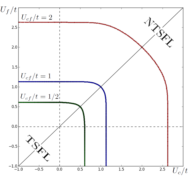
Figure 1: Phase diagram at half filling for $U_{cf}/t=\{1/2,1,2\}$. Inside the curves (at smaller values of $U_{\sigma}$) the TSFL phase occurs, while outside one has the NTSFL phase. As $U_{cf}/t$ increases, the zone of the TSFL phase becomes larger.

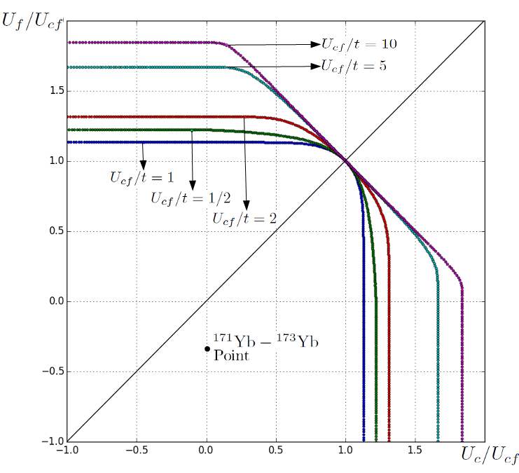
Figure 2: Phase diagram in units of $U_{cf}$ at half filling. The point $U_{c}=U_{f}=U_{cf}$ is a transition point between the phases TFSL and NTFSL, irrespectively of the value for $t$. It is also depicted the point representing the natural interactions of the mixture ${}^{171}\mathrm{\mathrm{Yb}}$-${}^{173}\mathrm{\mathrm{Yb}}$ yip2011 . The corresponding estimates for this point are performed in Sec. V.

IV.1 Attractive $U_{c}$, $U_{f}$

The results presented in Fig. 1 refer to the the half-filling case ($n_{\sigma}=\frac{1}{2}$, corresponding to $n_{c}=n_{f}\equiv n=1$) and different values of the ratio $U_{cf}/t$ and $U_{c}/t$, $U_{f}/t$. In this case we always find $\tilde{\mu}_{\sigma}=0$, as required by particle-hole symmetry (see e.g. fradkin2013 ).

For each fixed value of $U_{cf}/t>0$ (attractive regime) a colored curve is drawn, separating the TSFL phase inside of it from the NTSFL phase outside. We see that, as we increase the value of $U_{cf}/t$, higher values of attractive intra-pair couplings $U_{c}/t$, $U_{f}/t$ are required to break the TFSL phase in favour of the NTSFL one. At variance the normal state is never favored over both the superfluid states, even when one of or both the intra-pair interactions are repulsive and not small in comparison with the attractive ones. In this case the mean field approach is expected not to be reliable and, as we will see in the next Subsection, antiferromagnetic states can be instead favoured.

In Fig. 2 the curves of Fig. 1 are rescaled by their values of $U_{cf}/t$: in this way they all meet in the point $U_{c}=U_{f}=U_{cf}$. In this point all the different Hamiltonians have a $U\left(4\right)$ symmetry and the two phases TFSL and NTFSL can be mapped onto each other, signaling a transition point between the two phases, in agreement with lepori2015 .

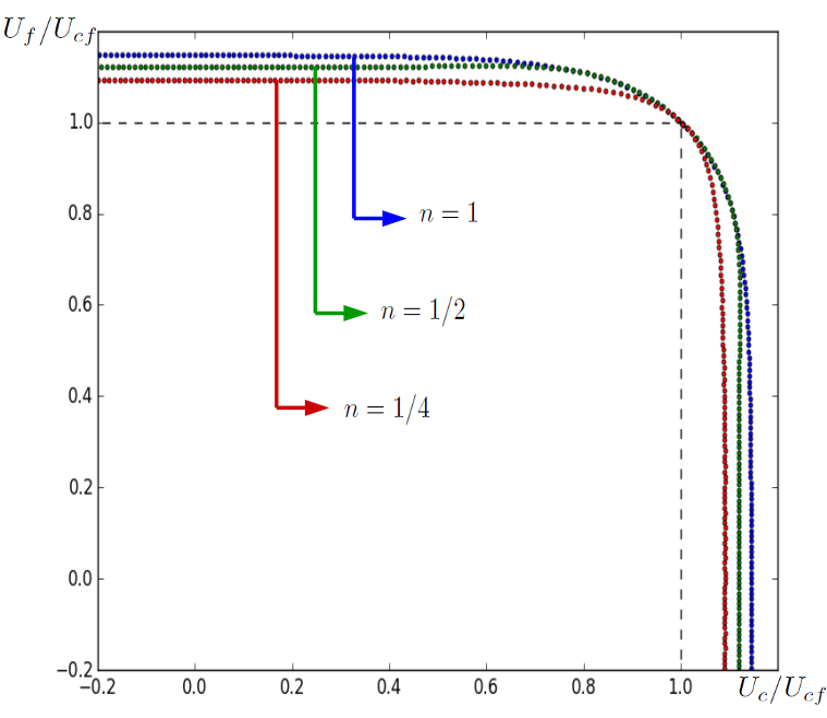
Figure 3: Phase diagrams for $U_{cf}/t=1$ and for different fillings: $n=1$ (blue), $n=1/2$ (green) and $n=1/4$ (red). They appear qualitatively very similar indicating that the filling does not play a fundamental role.

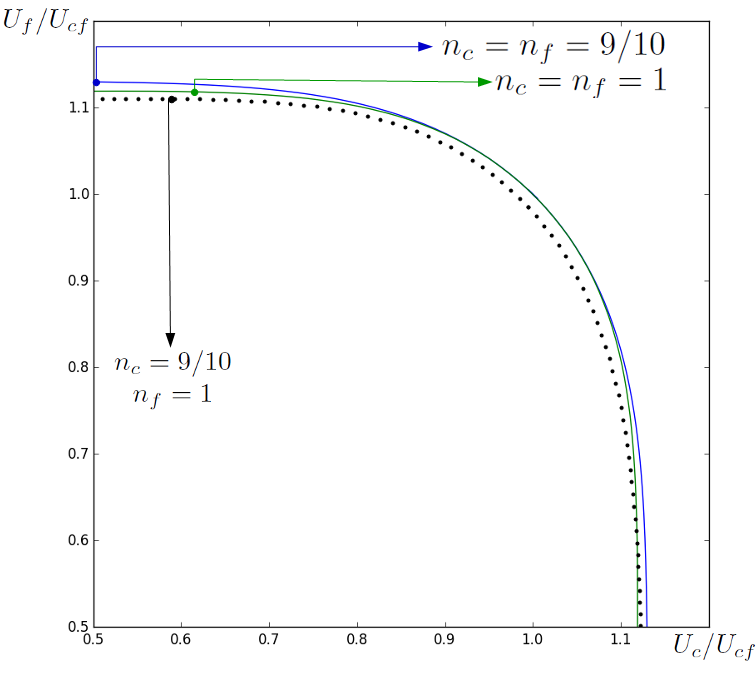
Figure 4: Phase diagram in the presence of a small unbalance between the populations $n_{f}-n_{c}=0.1$ and $U_{cf}=t$. The result is qualitatively very similar to the balanced cases (see also Figs. 2 and 3).

The black point in Fig. 2 represents the case of the mixture composed by ${}^{171}\mathrm{\mathrm{Yb}}$ and ${}^{173}\mathrm{\mathrm{Yb}}$, where natural interactions between these isotopes are also assumed. This mixture, mentioned in Section I, will be discussed in detail in Section V. Here we notice only that the point lies well inside the TSFL zone.

The phase diagram shown in Fig. 2 is not a consequence of the hypothesis of balanced mixture. Indeed in Fig. 3 we plot the same phase diagram for different fillings (but still equal for the four $\sigma$ species), finding qualitative agreements with small quantitative differences. Similarly, in Fig. 4 the case where the pairs $c$ and $f$ have fillings differing by ten percent is reported. Again we see that the imbalance in the populations does not produce significative differences on the results. We stress that, although an imbalance in the number of particles is generally known able to spoil the appearance of superfluid states pethick , in the present case the reliability of our results is guaranteed by the absence of other non-trivial solutions for the Eqs. (8) (see for comparison, e.g., mannarelli2006 ) and by the direct comparison between the energies of the normal states and the one of the BCS-like superfluid solutions.

IV.2 Repulsive $U_{c}$, $U_{f}$

When $U_{c}$, $U_{f}$ assume negative values and repulsive intra-pair interactions appear in the Hamiltonian of Eq. (1), the formation of intra-pair pairs start to become suppressed. However the normal state is never favored in the mean field approximation as shown in Figs. 1-4.

If it is reasonable that for small intra-pair repulsions the TSFL is favoured, for large enough values of $U_{c}/t$, $U_{f}/t$ and $U_{c}/U_{cf}$, $U_{f}/U_{cf}$ this superfluid phase is expected to eventually disappear, replaced by insulator phases with a magnetic-like order. The latter regime is qualitatively described in the strong coupling limit $U_{c}/t$, $U_{f}/t$ by spin Hamiltonians, similarly to the Heisenberg model for a two species repulsive mixtures at half filling (see, e.g., fradkin2013 ).

In the strong-coupling limit two cases are explicitly considered here: $a)$ $|U_{c}|/t,|U_{f}|/t\gg 1$, $b)$ $|U_{c}|/t\ll 1$ and $|U_{f}|/t\gg 1$. Notice that in both cases the further condition $|U_{c}/U_{cf}|,|U_{f}/U_{cf}|\gg 1$ is implicitly assumed.

In the first case the strong coupling Hamiltonian reads (details of the derivation are in the Appendix A):

$$\hat{H}^{cf}_{eff}=\frac{t^{2}}{4}\underset{\left\langle i,j\right\rangle}{\sum}\left(\frac{1}{\left|U_{c}\right|}\vec{C}_{i}\cdotp\vec{C}_{j}+\frac{1}{\left|U_{f}\right|}\vec{F}_{i}\cdotp\vec{F}_{j}\right)-E_{GS}^{cf},$$ (12)

where $\vec{C}$ and $\vec{F}$ are effective spin variables defined by $\vec{S}_{i}=\underset{\sigma\sigma^{\prime}}{\sum}c_{i\sigma}^{\dagger}\vec{\tau}_{\sigma\sigma^{\prime}}c_{i\sigma^{\prime}}$ ($\vec{\tau}$ denoting the Pauli matrices) and $E_{GS}^{cf}$ is the ground-state energy given by

$$E_{GS}^{cf}=-NU_{cf}-\frac{zNt^{2}}{4}\left(\frac{1}{\left|U_{c}\right|}+\frac{1}{\left|U_{f}\right|}\right),$$ (13)

where $N=2V$ is the total number of atoms of each pair. The Hamiltonian in Eq. (12) corresponds to two decoupled Heisenberg models.

The case $b)$ is of interest for the $\mathrm{Yb}$ discussed in the next Section, in the perspective of a possible experimental realization for the TFSL mechanism. Here the ground-state energy is found in the limit $U_{c}/t\to 0$ (see details in Appendix B):

$$E_{GS}^{c}=2E_{GS}^{NS}+\Delta E=2E_{GS}^{NS}-N\left(\frac{U_{c}}{4}+\frac{z\,t^{2}}{4\left|U_{f}\right|}\right),$$ (14)

where $E_{GS}^{NS}$ is the energy of a single $c$ component in the normal state. Indeed the energy in Eq. (14) is proper of a system of free fermions $c$ on a antiferromagnetic background describing the dynamics of the $f$ fermions and described by a spin Hamiltonian similar to the one in Eq. (12).

The regions of the phase diagram where both the TFSL and NTSFL superfluid phases occur can be bounded comparing their ground-state energies with the energies of the antiferromagnetic phases in Eqs. (13) and (14).

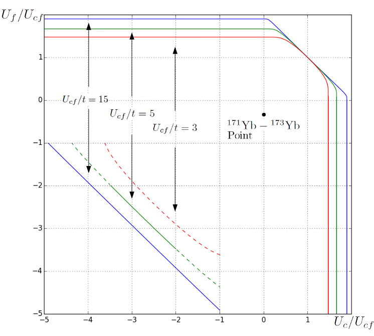
Figure 5: Phase diagram, containing the natural point for the Ytterbium mixture, for the cases $U_{cf}=3t$ (red), $U_{cf}=5t$ (green) and $U_{cf}=15t$ (blue). The oblique lines bounding the superfluid phases are obtained by the strong coupling approach leading to Eqs. (13) and (14). The transition from solid lines to dashed lines signals where this approach is not reliable any longer because it does not hold $|U_{c}/t|,|U_{f}/t|\gg 1$.

Postponing the details for the case $b)$ to the Section V, we presente the results of this calculation for the case $a)$ in Fig. 5. There the oblique lines represent a set of points where, according to the energy criterium mentioned above, the insulator states become favorable over the superfluid phases. Notice that increasing the depth $V_{0}$ results in a increase of the area of the TSFL phase, compared with the insulator one.

The calculation leading to Eqs. (13) and (14) is perturbative in $t/U_{\sigma}$, therefore the comparison between the energies in the same equations and the ones for the superfluid states is reliable only $t/U_{\sigma}\ll 1$. For this reason a dashed line, instead of a solid one, is drawn in Fig. 5 where the condition $|t/U_{\sigma}|>10^{-1}$ (a threshold conventionally chosen) starts to hold, so that the strong-coupling approach is no longer expected to be fully reliable. From the figure we see that for $U_{cf}/t=3$ the transition line can never be located perturbatively, while for $U_{cf}/t=15$ the converse is true. As an intermediate example $U_{cf}/t=5$ exhibits both a zone where perturbation theory can be assumed valid and other ones where it cannot.

V Experimental feasibility and limits

As mentioned in the Introduction, a possible experimental realization of the system investigated in the last Section is provided by a mixture of ${}^{171}\mathrm{\mathrm{Yb}}$ and ${}^{173}\mathrm{Yb}$. The first isotope has a $1/2$ hyperfine multiplet while the second one has $5/2$ hyperfine degeneracy. For the latter atomic species only two levels could be selectively populated. The mixture obtained in this way exhibits natural interactions characterized as follows: using conventionally the label $c$ for the hyperfine levels of ${}^{171}\mathrm{Yb}$ and the label $f$ for the ones of ${}^{173}\mathrm{Yb}$, the scattering lengths are $a_{c}=-3a_{0}$, $a_{f}=200a_{0}$ and $a_{cf}=-578a_{0}$, where $a_{0}$ is the Bohr radius (see e.g. taie2010 ; yip2011 ). As in all the earth-alkaline atoms, the tunability of these interactions is very difficult using the magnetic Feshbach resonance, because of the negligible magnetic moment of such atoms. Moreover, in the recent literature this problem revealed challenging also using alternative techniques, due to important atomic losses and without spoiling their characteristic $U(N)$ invariance ($N$ denoting here the number of hyperfine levels of the considered atomic species). For details on this subject see pagano2015 and references therein. This problem can prevent the realization of certain phases and the exploration of the full phase diagram. For our purposes the question is then if without tuning the interaction the TSFL superfluid phase is realized or not.

For the considered earth-alkaline mixture loaded on a cubic lattice, the hopping parameters, in principle different, are given by:

$$\begin{gathered}t_{\alpha}=-\int d^{3}\vec{r}\,\Bigg{(}\frac{\hbar^{2}}{2m_{\alpha}}\nabla\phi_{\alpha\vec{r}^{\prime}}\left(\vec{r}\right)\cdot\nabla\phi_{\alpha\vec{r}^{\prime\prime}}\left(\vec{r}\right)+\\ +\,\phi_{\alpha\vec{r}^{\prime}}\left(\vec{r}\right)V_{\mathrm{ext}}\left(\vec{r}\right)\phi_{\alpha\vec{r}^{\prime\prime}}\left(\vec{r}\right)\Bigg{)}.\end{gathered}$$ (15)

The expressions for the interaction parameters $U_{c},U_{f},U_{cf}$ in the form of $U_{\alpha\beta}$ for $\alpha\neq\beta\in\left\{r,g,u,d\right\}$ are [notice the minus sign in (1)]:

$$U_{\alpha\beta}=-\frac{\pi\hbar^{2}a_{\alpha\beta}}{m_{\alpha\beta}}\int d^{3}\vec{r}\left|\phi_{\alpha\vec{r}^{\prime}}\left(\vec{r}\right)\right|^{2}\left|\phi_{\beta\vec{r}^{\prime}}\left(\vec{r}\right)\right|^{2}.$$ (16)

In Eqs. (15) and (16), $\phi_{\{\alpha,\beta\}\vec{r}^{\,\prime}}\left(\vec{r}\right)$ are the Wannier functions describing the localization on a given lattice site $\vec{r}^{\,\prime}$ (these labels are suppressed in the following for sake of brevity), $\vec{r}$ is the distance from a chosen site, and $m_{\alpha\beta}=\frac{m_{\alpha}\,m_{\beta}}{m_{\alpha}+m_{\beta}}$. A simple variational estimate for the Wannier functions, which results in an estimate for the parameters in Eqs. 15 and 16, is discussed in Appendix C.

The tight binding regime for the $\mathrm{Yb}$ is achieved for $V_{0}\gtrsim 2-3E_{R_{c}}$ where $E_{Rc}=\frac{\hbar^{2}k_{0}^{2}}{2m}$ is the recoil energy, $k_{0}$ is the wave vector of the laser producing the optical lattice and $m$ is chosen conventionally to be the mass of the ${}^{171}\mathrm{Yb}$ isotope. We consider $V_{0}$ up to $\approx 15E_{R_{c}}$, where the tunneling coefficients are very small and tunneling dynamics effectively suppressed. Assuming this interval for the ratio $V_{0}/E_{R_{c}}$ and Eqs. (15) and (16) with their optimized Wannier wavefunctions, the regions on the diagram $U_{c}/U_{cf}$, $U_{f}/U_{cf}$ associated with the considered $\mathrm{Yb}$ mixture with natural interactions can be calculated.

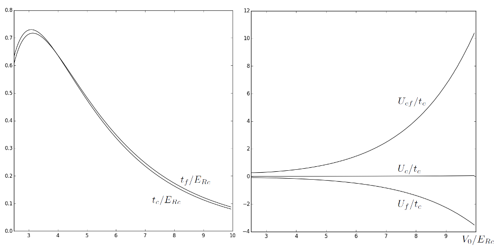
Figure 6: Parameters of the Hamiltonian in Eq. (1) as a function of the depth of the optical lattice potential $\tilde{V}_{0}=V_{0}/E_{Rc}$. Left panel: hopping parameters $t_{c}/E_{Rc}$ and $t_{f}/E_{Rc}$. Right panel: rescaled interaction parameters $U_{c,f}/t_{c}$ and $U_{cf}/t_{c}$.

In Fig. 6 we report on the left panel the hopping coefficients for different rescale depths $\tilde{V}_{0}=V_{0}/E_{Rc}$. We see in the left panel that, also considering the small difference in mass between the two isotopes, it always holds $\Delta t/t\lesssim 10^{-1}$ so that the previous assumption $t_{c}=t_{f}\equiv t$ (however not strictly required for the TFSL mechanism) is reasonable. On the right panel of the same figure we report the variation of $U_{\alpha,\beta}/t$, again as functions of $\tilde{V}_{0}=V_{0}/E_{Rc}$. In the same way, the region in the diagram $U_{c,f}/U_{cf}$ associated with the $\mathrm{Yb}$ mixture can be also calculated. More details on the calculation are given in Appendix C.

We observe that, once the intra-pair interactions are written in the form $U_{c,f}/U_{cf}$, the dependence on the amplitude $V_{0}$ effectively drops out, such that only the relative value of $U_{cf}/t$ changes significantly and the obtained region resembles a single point. This is the reason why we can speak about just a ”natural point’ in the diagrams of Figs. 2 and 5. This point is given approximately by the coordinates $U_{c}/U_{cf}\approx 0.01$ and $U_{f}/U_{cf}\approx-0.34$, also very close to the point estimated using the approximation $U_{\alpha}/U_{cf}\simeq a_{\alpha}/a_{cf}$ valid in the continuous space limit.

Importantly the natural point falls well inside the TSFL regime, see Figs. 2 and 5. In particular, along the line $U_{c}/t=0$ (case $b$ in Section IV), where the point almost lies, an estimate for the appearance of the antiferromagnetic regime can be done comparing the energies in Eqs. (6) and (14). As a result, the transition is located by the strong coupling approach at the values $U_{c}/U_{cf}=-3.97$ for $U_{cf}/t=3$, $U_{c}/U_{cf}\approx-4.9$ for $U_{cf}/t=5$ and $U_{c}/U_{cf}\approx-5.6$ for $U_{cf}/t=15$, in all the three cases far from the natural point of the $\mathrm{Yb}$. In this way, our findings indicate that the TSFL phase can be observed in the zero temperature limit in experiments with $\mathrm{Yb}$ mixtures, assuming natural interactions and realistic values for the depth of the lattice potential.

Despite of the zero-temperature results reported, the TSFL phase could be still unreachable in the presence of a too low critical temperature (at fixed interactions) required for its emergence, in comparison with the ones currently realizable. This point is particular important in the light of the mentioned difficulty to tune the interactions in earth-alkaline atoms. We can make an estimate of the critical temperature for the $\mathrm{Yb}$ mixture. Proceeding as for the two-component attractive Hubbard model iazzi2012 , in the present case we refer to the case of isotropic hoppings $t$ ($t_{\perp}=t_{\parallel}=t$ in the notation of iazzi2012 ) and to the half filling case. Moreover $\tilde{\mu}_{c}=\tilde{\mu}_{f}$, as we found in Section III.

For our model on a cube lattice the total bandwidth is $D=12t$. If we consider for instance $V_{0}=5E_{Rc}$, we obtain $2U_{cf}\approx 0.3D$, which results in $T_{c}K_{B}/D\approx 0.05$. Using these values and considering a lattice spacing of $a=0.5\,\mu m$, the critical temperature turns out $T_{c}\approx 15\ \mathrm{nK}$. In terms of the Fermi temperature this amounts to obtain $T_{c}/T_{F}\approx 0.1$. This value is reasonably close to the ones achievable in current experiments valtolina15 , suggesting that the critical temperature assuming the natural interaction is reachable with current-day experiments and the TSFL phase could be achieved.

The lattice ratio $T_{c}/T_{F}\approx 0.1$ can be compared with the typical one for experiments in the continuous space, finding that apparently on the lattice $T_{c}/T_{F}$ is sensibly larger. Indeed a very simple estimate can be done using the results varenna2006 for a two-component mixture (as it is effectively the TSFL phase). Considering a number of loaded atoms $N\approx 10^{4}$ and a system size $\ell\sim 10\mu m$, one obtains $T_{c}/T_{F}$ smaller than $0.01$. This value is far from the presently achievable ones, differently from the lattice case. Summing up, the present analysis suggests that, for the task to synthesize a TFSL phase in $\mathrm{Yb}$ mixtures, the use of a (cubic) lattice can be advantageous.

VI Conclusions

In this paper we investigated the possible emergence of a non-Abelian two-flavor locking (TSFL) superfluid phase in ultracold Fermi mixtures with four components and unequal interactions. More in detail, using mean field and strong coupling results, we explored the phase diagram of this mixture loaded in a cubic lattice, finding for which ranges of the interactions and of the lattice width the system exhibits a TSFL phase.

These ranges are found to have an extended overlap with the ones realizable in current experiments. In particular, as detailed in the text, the proposed set-up and phase are found to be realistic and realizable using a mixture of ${}^{171}\mathrm{Yb}$ and ${}^{173}\mathrm{Yb}$. The phase diagram has been studied and the point in the phase diagram associate to the natural (not tuned) interactions between these atomic species determined. The critical temperature required for the appearance of the TSFL superfluid has been found comparable with the ones currently achievable. The latter ingredient is central for a possible experiment aiming to realize the TFSL phase, especially due to the known difficulty to tune interactions in earth-alkaline atomic gases, without spoiling their peculiar $U(N)$ invariance.

We finally observe that for our results it is crucial that relative large intra-pair repulsions do not destroy the superfluid states. Different is expected to be the case where non-local repulsive interactions are present, whose effects can be considered an interesting subject of future work.

Appendix A $c$ and $f$ strongly coupled limit

In this Appendix we present details of the perturbative calculation for the strongly coupled limit in the presence of repulsive intra-pair interactions, leading to Eq. (12) in the main text. We consider half filling.

The described physical situation corresponds to consider the Hamiltonian $H_{0}+H_{1}$

$$H_{0}=2\underset{i}{\sum}\left(|U_{c}|n_{ir}n_{ig}+|U_{f}|n_{iu}n_{id}\right)-2|U_{cf}|\underset{i,c,f}{\sum}n_{ic}n_{if},$$ (17)

$$H_{1}=-t\underset{\left\langle i,j\right\rangle,\sigma}{\sum}c_{i\sigma}^{\dagger}c_{j\sigma},$$ (18)

and perform perturbation theory in the parameters $\varepsilon_{c},\varepsilon_{f}\ll 1$ with $\varepsilon_{c}=t/|U_{c}|,\varepsilon_{f}=t/|U_{f}|$. We assume $\varepsilon_{c}=\varepsilon_{f}=\varepsilon$. The ground-states of $H_{0}$, with energies $E=-2V|U_{cf}|=-N|U_{cf}|$, are the states where no single site is doubly occupied by intra-pairing atoms, provided that $\left|U_{c,f}\right|>3/2\,|U_{cf}|$. Let $\hat{G}$ be the projector on this space and $\hat{P}=1-\hat{G}$.

The lowest order correction to $E$ comes at the second order, from the virtual process consisting in the interchange of location of two particles at nearest-neighbour distance. The calculation simplifies once we note that $\hat{P}H_{1}=H_{1}$ and that $H_{1}\left|\phi\right\rangle$ is an eigenvector of $H_{0}$ for $\left|\phi\right\rangle$ a ground-state. The related second order effective Hamiltonian then is found to be

$$H_{eff}=\frac{t^{2}}{4}\underset{\left\langle i,j\right\rangle}{\sum}\left(\frac{1}{\left|U_{c}\right|}\vec{C}_{i}\cdotp\vec{C}_{j}+\frac{1}{\left|U_{f}\right|}\vec{F}_{i}\cdotp\vec{F}_{j}\right)-\\ -\frac{zNt^{2}}{8}\left(\frac{1}{\left|U_{c}\right|}+\frac{1}{\left|U_{f}\right|}\right),$$ (19)

where $\vec{C}$ and $\vec{F}$ are the associated spin variables defined by $\vec{S}_{i}=\underset{\sigma\sigma^{\prime}}{\sum}c_{i\sigma}^{\dagger}\vec{\tau}_{\sigma\sigma^{\prime}}c_{i\sigma^{\prime}}$. The corresponding ground-state energy correction is $\Delta E=-\frac{zNt^{2}}{4}\left(\frac{1}{\left|U_{c}\right|}+\frac{1}{\left|U_{f}\right|}\right)$, being $z$ the adjacency number for every site. In this way the ground-state energy at the second order perturbation theory in $\frac{t}{U_{c,f}}$ becomes

$$E=-N|U_{cf}|-\frac{zNt^{2}}{4}\left(\frac{1}{\left|U_{c}\right|}+\frac{1}{\left|U_{f}\right|}\right).$$ (20)

This formula appears in Eq. (13) in the main text.

Appendix B Strongly coupled $f$ and weakly coupled $c$

In this case the system is described by the Hamiltonian (in the same notation of Appendix A) $H_{0}+H_{1}+H_{2}$, with:

$$H_{0}=2|U_{f}|\underset{i}{\sum}\hat{n}_{iu}\hat{n}_{id}-2|U_{cf}|\underset{i,c,f}{\sum}\hat{n}_{ic}\hat{n}_{if}-t\underset{\left\langle i,j\right\rangle,c}{\sum}c_{ic}^{\dagger}c_{jc},$$ (21)

$$H_{1}=-t\underset{\left\langle i,j\right\rangle,f}{\sum}\,c_{if}^{\dagger}c_{jf}\,,\quad\quad H_{2}=-2U_{c}\underset{i}{\sum}n_{ir}n_{ig},$$ (22)

and the perturbative parameters are $\varepsilon_{1}=\frac{t}{|U_{f}|}$ and $\varepsilon_{2}=\frac{|U_{c}|}{t}$. The ground-state of $H_{0}$ can be derived in this limit assuming a basis of localized $f$ degrees of freedom. Using such a basis, we can get an effective Hamiltonian for the $c$ degrees of freedom corresponding to non-interacting fermions in a one body potential, in turn depending on the $f$ configuration.

If $\left|U_{f}\right|\gg t$ and $\left|U_{f}\right|\gg|U_{cf}|$, the dynamics is dominated by the localization of the $f$ atoms and therefore the ground-state does not host any doubly occupied site. In that case in the ground state of $H_{0}$, a single $f$ particle is in each site, therefore the one-body potential felt by the $c$ particles is site independent: $-2\left|U_{cf}\right|\hat{n}_{ic}$. The effect of this potential is to induce a shift $\delta\mu_{c}=-2\,|U_{cf}|$. Up to the first order of perturbation, the ground-state energy then results of $E_{0c}=2\underset{\vec{k}:\varepsilon_{\vec{k}}<0}{\sum}\,\varepsilon_{\vec{k}}$. Instead the first order in $\epsilon_{1}$ vanishes because it is related with forbidden double occupancies of sites by particles of the same species.

At the second order in $\varepsilon_{1}$ and $\varepsilon_{2}$, an effective Hamiltonian can be derived:

$$\hat{H}_{eff}=\hat{G}\Bigg{[}\varepsilon_{1}^{2}\hat{H}_{1}\frac{1}{\left(E_{0}-\hat{H}_{0}\right)}\hat{P}\hat{H}_{1}+\\ \varepsilon_{1}\varepsilon_{2}\left(\hat{H}_{1}\frac{1}{\left(E_{0}-\hat{H}_{0}\right)}\hat{P}\hat{H}_{2}+\mathrm{h.c.}\right)+\\ +\,\varepsilon_{2}^{2}\hat{H}_{2}\frac{1}{\left(E_{0}-\hat{H}_{0}\right)}\hat{P}\hat{H}_{2}\Bigg{]}\hat{G}\,,$$ (23)

wit $\hat{G}$ and $\hat{P}=1-\hat{G}$ as before. The term $\propto\epsilon_{1}\epsilon_{2}$ vanishes for the same reason for which the linear term in $\epsilon_{1}$ does, and the remaining effective terms are then proportional to $\varepsilon_{2}$, $\varepsilon_{1}^{2}$ and $\varepsilon_{2}^{2}$. These terms commute with each other, so we can focus on them individually. After some algebra we arrive to the energy correction up to the second order for the ground-state energy:

$$\Delta E=N\left(-\frac{U_{c}}{4}-\frac{zt^{2}}{4}\left|U_{f}\right|-\frac{U_{c}^{2}}{t}\tilde{E}^{\left(2\right)}\right),$$ (24)

where $\tilde{E}^{\left(2\right)}$ is a dimensionless positive quantity:

$$\tilde{E}^{\left(2\right)}=-\frac{1}{V^{3}}\underset{\begin{array}[]{c}\vec{k_{1}},\vec{k_{2}}\in\mathbb{F}_{S}\\ \vec{q_{1}},\vec{q_{2}}\notin\mathbb{F}_{S}\end{array}}{\sum}\frac{\delta_{\vec{k_{1}}+\vec{k_{2}}\vec{q_{1}}+\vec{q_{2}}}}{\tilde{\varepsilon}_{\vec{k_{1}}}+\tilde{\varepsilon}_{\vec{k_{2}}}-\tilde{\varepsilon}_{\vec{q_{1}}}-\tilde{\varepsilon}_{\vec{q_{2}}}},$$ (25)

with $\mathbb{F}_{S}$ labelling the set of points of the Fermi sea and $\tilde{\varepsilon_{k}}=\varepsilon_{k}/2t$. Eq. (25) is used to arrive to Eq. (14) of the main text, where $U_{c}=0$ and it is not needed to calculate $\tilde{E}^{\left(2\right)}$.

Appendix C Determination of the model parameters

In the present Appendix we perform a variational estimate of the parameters entering in the Hamiltonian 1, which can be obtained from the expressions

$$\begin{gathered}t_{ij\alpha}=-\int d^{3}\vec{r}\,\Bigg{(}\frac{\hbar^{2}}{2m_{\alpha}}\nabla\phi_{i\alpha}\left(\vec{r}\right)\cdot\nabla\phi_{j\alpha}\left(\vec{r}\right)+\\ +\,\phi_{i\alpha}\left(\vec{r}\right)V_{\mathrm{ext}}\left(\vec{r}\right)\phi_{j\alpha}\left(\vec{r}\right)\Bigg{)},\\ {}\\ U_{\alpha\beta}=-\frac{\pi\hbar^{2}a_{\alpha\beta}}{m_{\alpha\beta}}\int d^{3}\vec{r}\left|\phi_{\alpha}\left(\vec{r}\right)\right|^{2}\left|\phi_{\beta}\left(\vec{r}\right)\right|^{2}.\end{gathered}$$ (26)

$V_{\mathrm{ext}}\left(\vec{r}\right)=V_{0}\underset{j=1}{\overset{3}{\sum}}\sin^{2}\left(k_{0}r_{i}\right)$ is the external potential creating the lattice ($k_{0}=\frac{2\pi}{a}$, $a$ being the lattice spacing), $a_{\alpha\beta}$ correspond to the scattering lengths between the $\alpha$ and $\beta$ species, and $m_{\alpha\beta}$ are their reduced masses. Moreover the $\phi_{\alpha}\left(\vec{r}\right)$ refer to the Wannier functions centered on the lattice sites. A simple estimate of these functions can be obtained by variational approach. In particular we consider the following ansatz:

$$\phi_{\alpha}\left(\vec{r}\right)=C_{\alpha}e^{-\frac{|\vec{r}|^{2}}{2\sigma_{\alpha}^{2}}},$$ (27)

where $C_{\alpha}=\left(\sqrt{\pi}\sigma_{\alpha}\right)^{-3/2}$ and the coefficients $\sigma_{\alpha}$ are fixed minimizing the energy per lattice site. This value can be found as the expectation value of the Hamiltonian (1) acting on the multi-particles fermionic state $\Psi_{\alpha}(\vec{r}_{1},\dots,\vec{r}_{V})$ ($V$ being the number of lattice sites, at half filling equal to the number of $c$ or $f$ atoms) constructed by the Wannier functions. In the mean field approximation it reads:

$$\varepsilon=\int\prod_{i=1}^{V}\,d^{3}\vec{r}_{i}\Bigg{(}\underset{\alpha}{\sum}\frac{\hbar^{2}}{2m_{\alpha}}\left|\nabla\Psi_{\alpha}\right|^{2}+V_{ext}\left|\Psi_{\alpha}\right|^{2}+\\ +\,\underset{\beta>\alpha}{\sum}\frac{2\pi\hbar^{2}a_{\alpha\beta}}{m_{\alpha\beta}}\left|\Psi_{\alpha}\right|^{2}\left|\Psi_{\beta}\right|^{2}\Bigg{)}.$$ (28)

Using the (approximate) orthogonality of the Wannier functions at different lattice sites one obtains:

$$\varepsilon=\int d^{3}\vec{r}\,\underset{\vec{r}^{\prime},\alpha}{\sum}\Bigg{(}n_{\alpha}\frac{\hbar^{2}}{2m_{\alpha}}\left|\nabla\phi_{\alpha\vec{r}^{\prime}}\right|^{2}+n_{\alpha}V_{ext}\left|\phi_{\alpha\vec{r}^{\prime}}\right|^{2}+\\ +\,\underset{\beta>\alpha}{\sum}n_{\alpha}n_{\beta}\frac{g_{\alpha\beta}}{2}\left|\phi_{\alpha\vec{r}^{\prime}}\right|^{2}\left|\phi_{\beta\vec{r}^{\prime}}\right|^{2}\Bigg{)},$$ (29)

$n_{\{\alpha,\beta\}}$ being the average number of particles of $\{\alpha,\beta\}$ per site and $g_{\alpha\beta}=\frac{4\pi\hbar^{2}a_{\alpha\beta}}{m_{\alpha\beta}}$. Moreover the Wannier functions, centered on the lattice sites labelled by $\vec{r}^{\,\prime}$, depend on the space vector $\vec{r}$ spanning all the lattice. Using the ansatz in Eq. (27) one finds

$$\varepsilon/N=\underset{\alpha}{\sum}\Bigg{[}n_{\alpha}\frac{\hbar^{2}}{2m_{\alpha}}\frac{3}{2\sigma_{\alpha}^{2}}+n_{\alpha}\frac{3V_{0}}{2}\left(1-e^{-k_{0}^{2}\sigma_{\alpha}^{2}}\right)+\\ +\,\underset{\beta>\alpha}{\sum}n_{\alpha}n_{\beta}\frac{g_{\alpha\beta}}{2\pi^{3/2}\left(\sigma_{\alpha}^{2}+\sigma_{\beta}^{2}\right)^{3/2}}\Bigg{]}.$$ (30)

Imposing $\frac{\partial\varepsilon}{\partial\sigma_{\mu}}=0$ and expressing the parameters in Eq. (30) as adimensional quantities $\tilde{\sigma}_{\mu}=k_{0}\sigma_{\mu}$, $\tilde{V}_{\alpha}=\frac{V_{0}}{E_{R}^{\alpha}}$ and $\tilde{a}_{\alpha\beta}=k_{0}a_{\alpha\beta}$, with $E_{R}^{\alpha}=\frac{\hbar^{2}k_{0}^{2}}{2m_{\alpha}}$, the result is a set of coupled equations:

$$\frac{1}{\tilde{\sigma}_{\mu}^{3}}-\tilde{V}_{\mu}\tilde{\sigma}_{\mu}e^{-\tilde{\sigma}_{\mu}^{2}}+4\underset{\beta\neq\mu}{\sum}n_{\beta}\left(1+\frac{m_{\mu}}{m_{\beta}}\right)\frac{\tilde{a}_{\mu\beta}\tilde{\sigma}_{\mu}}{\sqrt{\pi}\left(\tilde{\sigma}_{\mu}^{2}+\tilde{\sigma}_{\beta}^{2}\right)^{5/2}}\,=0.$$ (31)

Solving this set in $\left\{\sigma_{\alpha}\right\}$, the Hubbard coefficients are finally obtained:

$$\begin{array}[]{c}t_{\alpha}=-\left[\frac{\hbar^{2}}{2m_{\alpha}}\frac{1}{4\sigma_{\alpha}^{2}}\left(6-\left(\frac{a}{\sigma_{\alpha}}\right)^{2}\right)+\frac{V_{0}}{2}\left(3-e^{-k_{0}^{2}\sigma_{\alpha}^{2}}\right)\right]e^{-\frac{a^{2}}{4\sigma_{\alpha}^{2}}},\\ \\ {}\hfil\\ U_{\alpha\beta}=-\frac{\hbar^{2}a_{\alpha\beta}}{\sqrt{\pi}m_{\alpha\beta}}\frac{1}{\left(\sigma_{\alpha}^{2}+\sigma_{\beta}^{2}\right)^{3/2}}.\end{array}$$ (32)

For the case of the $\mathrm{Yb}$ mixture the interactions are the same for the species $r,g$ and $u,d$, resulting in two equations (for $\tilde{\sigma_{c}}$ and $\tilde{\sigma_{f}}$):

$$\left\{\begin{array}[]{c}\frac{1}{\tilde{\sigma}_{c}^{3}}-\tilde{V}_{c}\tilde{\sigma}_{c}e^{-\tilde{\sigma}_{c}^{2}}+\frac{n_{c}\tilde{a}_{cc}}{\sqrt{2\pi}\tilde{\sigma}_{c}^{4}}+\left(1+\frac{m_{c}}{m_{f}}\right)\frac{4n_{f}\tilde{a}_{cf}\tilde{\sigma}_{c}}{\sqrt{\pi}\left(\tilde{\sigma}_{c}^{2}+\tilde{\sigma}_{f}^{2}\right)^{5/2}}=0\\ \\ \frac{1}{\tilde{\sigma}_{f}^{3}}-\tilde{V}_{f}\tilde{\sigma}_{f}e^{-\tilde{\sigma}_{f}^{2}}+\frac{n_{f}\tilde{a}_{ff}}{\sqrt{2\pi}\tilde{\sigma}_{f}^{4}}+\left(1+\frac{m_{f}}{m_{c}}\right)\frac{4n_{c}\tilde{a}_{cf}\tilde{\sigma}_{f}}{\sqrt{\pi}\left(\tilde{\sigma}_{c}^{2}+\tilde{\sigma}_{f}^{2}\right)^{5/2}}=0.\end{array}\right.$$ (33)

The solutions are presented in Fig. 6 of the main text for the symmetric case $n_{c}=n_{f}\equiv n=1$.

References

- (1) I. Bloch, J. Dalibard, and W. Zwerger, Rev. Mod. Phys. 80, 885 (2008).
- (2) M. Lewenstein, A. Sanpera, and V. Ahufinger, Ultracold atoms in optical lattices: simulating quantum many-body systems (Oxford, Oxford University Press, 2012).
- (3) J. Dalibard, F. Gerbier, G. Juzeliūnas, and P. Öhberg, Rev. Mod. Phys. 83, 1523 (2011).
- (4) M. Greiner, O. Mandel, T. Esslinger, T. W. Hänsch, and I. Bloch, Nature 415, 39 (2002).
- (5) J. Billy, V. Josse, Z. Zuo, A. Bernard, B. Hambrecht, P. Lugan, D. Clément, L. Sanchez-Palencia, P. Bouyer, and A. Aspect, Nature 453, 891 (2008).
- (6) G. Roati, C. D’Errico, L. Fallani, M. Fattori, C. Fort, M. Zaccanti, G. Modugno, M. Modugno, and M. Inguscio, Nature 453, 895 (2008).
- (7) F. S. Cataliotti, S. Burger, C. Fort, P. Maddaloni, F. Minardi, A. Trombettoni, A. Smerzi, and M. Inguscio, Science 293, 843 (2001).
- (8) T. Esslinger, Ann. Rev. Cond. Matt. Phys. 1, 129 (2010).
- (9) F. Gerbier and J. Dalibard, New J. Phys. 12, 033007 (2010).
- (10) E. Zohar, J. I. Cirac, and B. Reznik, Phys. Rev. Lett. 109, 125302 (2012); ibid. 110, 055302 (2013); ibid. 110, 125304 (2013).
- (11) D. Banerjee, M. Dalmonte, M. Müller, E. Rico, P. Stebler, U.-J. Wiese, and P. Zoller, Phys. Rev. Lett. 109, 175302 (2012).
- (12) L. Tagliacozzo, A. Celi, A. Zamora, and M. Lewenstein, Ann. Phys. 330, 160 (2013).
- (13) D. Banerjee, M. Bögli, M. Dalmonte, E. Rico, P. Stebler, U.-J. Wiese, and P. Zoller, Phys. Rev. Lett. 110, 125303 (2013).
- (14) M. J. Edmonds, M. Valiente, G. Juzeliūnas, L. Santos, and P. Öhberg, Phys. Rev. Lett. 110, 085301 (2013).
- (15) E. A. Martinez, C. A. Muschik, P. Schindler, D. Nigg, A. Erhard, M. Heyl, P. Hauke, M. Dalmonte, T. Monz, P. Zoller, and R. Blatt, Nature 534, 516 (2016).
- (16) N. Nagaosa, Quantum field theory in condensed matter physics (Berlin, Springer-Verlag, 1999).
- (17) L. Balents, Nature 464, 199 (2010).
- (18) P. A. Lee, N. Nagaosa, and X.-G. Wen, Rev. Mod. Phys. 78, 17 (2006).
- (19) D. Jaksch and P. Zoller, New J. Phys. 5, 56 (2003).
- (20) K. Osterloh, M. Baig, L. Santos, P. Zoller, and M. Lewenstein, Phys. Rev. Lett. 95, 010403 (2005).
- (21) M. Aidelsburger, M. Atala, S. Nascimbène, S. Trotzky, Y.-A. Chen, and I. Bloch, Phys. Rev. Lett. 107, 255301 (2011).
- (22) K. Jimenez-Garcia, L. J. Le Blanc, R. A. Williams, M. C. Beeler, A. R. Perry, and I. B. Spielman, Phys. Rev. Lett. 108, 225303 (2012).
- (23) P. Hauke, O. Tieleman, A. Celi, C. Ölschläger, J. Simonet, J. Struck, M. Weinberg, P. Windpassinger, K. Sengstock, M. Lewenstein, and A. Eckardt, Phys. Rev. Lett. 109, 145301 (2012).
- (24) S.-L. Zhu, B. Wang, and L.-M. Duan, Phys. Rev. Lett. 98, 260402 (2007).
- (25) B. Wunsch, F. Guinea, and F. Sols, New J. Phys. 10, 103027 (2008).
- (26) C. Wu and S. Das Sarma, Phys. Rev. B 77, 235107 (2008).
- (27) G. Juzeliūnas, J. Ruseckas, M. Lindberg, L. Santos, and P. Öhberg, Phys. Rev. A 77, 011802(R) (2008).
- (28) L.-K. Lim, C. M. Smith, and A. Hemmerich, Phys. Rev. Lett. 100, 130402 (2008).
- (29) J.-M. Hou, W.-X. Yang, and X.-J. Liu, Phys. Rev. A 79, 043621 (2009).
- (30) K. L. Lee, B. Grémaud, R. Han, B.-G. Englert, and C. Miniatura, Phys. Rev. A 80, 043411 (2009).
- (31) E. Alba, X. Fernandez-Gonzalvo, J. Mur-Petit, J. J. Garcia-Ripoll, and J. K. Pachos, Ann. Phys. 328, 64 (2013).
- (32) L. Lamata, J. Léon, T. Schätz, and E. Solano, Phys. Rev. Lett. 98, 253005 (2007).
- (33) L. Lepori, G. Mussardo, and A. Trombettoni, Europhys. Lett. 92, 50003 (2010).
- (34) L. Mazza, A. Bermudez, N. Goldman, M. Rizzi, M. A. Martin-Delgado, and M. Lewenstein, New. Journ. Phys. 14, 01500 (2012).
- (35) A. Bermudez, L. Mazza, M. Rizzi, N. Goldman, M. Lewenstein, and M. A. Martin-Delgado, Phys. Rev. Lett. 105, 190404 (2010).
- (36) Z. Lan, A. Celi, W. Lu, P. Öhberg, and M. Lewenstein, Phys. Rev. Lett. 107, 253001 (2011).
- (37) O. Boada, A. Celi, J. I. Latorre, and M. Lewenstein, Phys. Rev. Lett. 108, 133001 (2012).
- (38) O. Boada, A. Celi, M. Lewenstein, J. Rodr guez-Laguna, and J. I. Latorre, New Journ. of Phys. 17, 045007 (2015).
- (39) L. Lepori, A. Trombettoni, and W. Vinci, Europhys. Lett. 109, 50002 (2015).
-
(40)
V. Kasper, F. Hebenstreit, M. Oberthaler, and J. Berges,
arXiv:1506.01238 - (41) C. Laflamme, W. Evans, M. Dalmonte, U. Gerber, H. Mejía-Díaz, W. Bietenholz, U.-J. Wiese, and P. Zoller, Ann. Phys. 370, 117 (2016).
- (42) L. Tarruell, D. Greif, T. Uehlinger, G. Jotzu, and T. Esslinger, Nature 483, 302 (2012).
- (43) G. Jotzu, M. Messer, R. Desbusquois, M. Lebrat, T. Uehlinger, D. Greif, and T. Esslinger, Nature 515, 237 (2014).
- (44) The BCS-BEC Crossover and the Unitary Fermi Gas, W. Zwerger ed. (Heidelberg, Springer, 2012).
- (45) D. J. Dean and M. Hjorth-Jensen, Rev. Mod. Phys. 75, 607 (2003).
- (46) M. Alford, A. Schmitt, K. Rajagopal, and T. Schäfer, Rev. Mod. Phys. 80, 1455 (2008).
- (47) R. Anglani, R. Casalbuoni, M. Ciminale, R. Gatto, N. Ippolito, M. Mannarelli, and M. Ruggieri, Rev. Mod. Phys. 86, 509 (2014).
- (48) R. Auzzi, S. Bolognesi, J. Evslin, K. Konishi, and A. Yung, Nucl. Phys. B 673, 187 (2003).
- (49) R. Auzzi, S. Bolognesi, J. Evslin, K. Konishi, and H. Murayama, Nucl. Phys. B 701, 207 (2004).
- (50) M. Shifman and A. Yung, Phys. Rev. D 70, 045004 (2004).
- (51) A. Hanany and D. Tong, JHEP 07, 037 (2003).
- (52) M. Eto, Y. Isozumi, M. Nitta, K. Ohashi, and N. Sakai, Phys. Rev. Lett. 96, 161601 (2006).
- (53) M. Alford, K. Rajagopal, and F. Wilczek, Nucl. Phys. B 537, 443 (1999).
- (54) G. Pagano, M. Mancini, G. Cappellini, P. Lombardi, F. Schäfer, H. Hu, X.-J. Liu, J. Catani, C. Sias, M. Inguscio, and L. Fallani, Nature Phys. 10, 198 (2014).
- (55) A. V. Gorshkov, M. Hermele, V. Gurarie, C. Xu, P. S. Julienne, J. Ye, P. Zoller, E. Demler, M. D. Lukin and A. M. Rey, Nature Phys. 6, 289 (2010).
- (56) S. Taie, Y. Takasu, S. Sugawa, R. Yamazaki, T. Tsujimoto, R. Murakami, and Y. Takahashi, Phys. Rev. Lett. 105, 190401 (2010).
- (57) S.-K. Yip, Phys. Rev A 83, 063607 (2011).
- (58) C. J. Pethick and H. Smith, Bose-Einstein Condensation in Diluite Gases, 2nd ed., Chap. 16 (Cambridge, Cambridge University Press, 2008).
- (59) E. Fradkin, Field Theories of Condensed Matter Physics (Cambrdige, Cambridge University Press, 2013).
- (60) M. Mannarelli, G. Nardulli, and M. Ruggieri, Phys. Rev. A 74, 033606 (2006).
- (61) G. Pagano, M. Mancini, G. Cappellini, L. Livi, C. Sias, J. Catani, M. Inguscio, and L. Fallani, Phys. Rev. Lett. 115, 265301 (2015).
- (62) M. Iazzi, S. Fantoni, and A. Trombettoni, Europhys. Lett. 100 36007 (2012).
- (63) G. Valtolina, A. Burchianti, A. Amico, E. Neri, K. Xhani, J. A. Seman, A. Trombettoni, A. Smerzi, M. Zaccanti, M. Inguscio, and G. Roati, Science 350, 1505 (2015).
- (64) W. Ketterle and M. W. Zwierlein, Making, probing and understanding ultracold Fermi gases, in Ultracold Fermi Gases, Proceedings of the International School of Physics ”Enrico Fermi”, Course CLXIV, Varenna, 20 - 30 June 2006, M. Inguscio, W. Ketterle, and C. Salomon eds. (Amsterdam, IOS Press, 2008).