Inverse problem for multi-body interaction of nonlinear waves

Abstract

The inverse problem is studied in multi-body systems with nonlinear dynamics representing, e.g., phase-locked wave systems, standard multimode and random lasers. Using a general model for four-body interacting complex-valued variables we test two methods based on pseudolikelihood, respectively with regularization and with decimation, to determine the coupling constants from sets of measured configurations. We test statistical inference predictions for increasing number of sampled configurations and for an externally tunable temperature-like parameter mimicing real data noise and helping minimization procedures. Analyzed models with phasors and rotors are generalizations of problems of real-valued spherical problems (e.g., density fluctuations), discrete spins (Ising and vectorial Potts) or finite number of states (standard Potts): inference methods presented here can, then, be straightforward applied to a large class of inverse problems. The high versatility of the exposed techniques also concerns the number of expected interactions: results are presented for different graph topologies, ranging from sparse to dense graphs.

Multi-body inference turns out to be essential whenever non-linear response is crucial for a system properties. Light mode interaction in ultra-fast multimode lasers Sargent III et al. (1978); Haus (2000); Gordon and Fischer (2002); Katz et al. (2006); Antenucci et al. (2015a, b), random lasers Lawandy et al. (1994); Cao et al. (1998); Wiersma (2008); Antenucci et al. (2015c), multi-variable clause constrained problems Monasson and Zecchina (1997); Mézard et al. (2002), error correcting codes Kay" (2003); Mézard and Montanari (2009), effective interaction among density fluctuations in heterogeneous frustrated glassy systems Kirkpatrick et al. (1989); Crisanti and Sommers (1992); Götze (2009); Franz et al. (2011); Caltagirone et al. (2012); Ferrari et al. (2012) and fish shoals behavior Katz et al. (2011); Herbert-Read et al. (2011) are significant diverse examples of direct problems in which nonlinearity plays a non-perturbative role in determining the system behavior. Nevertheless, to our knowledge, not many studies of the inverse problem have been performed so far in the field. In this work we aim at filling in this gap presenting a detailed analysis based on pseudolikelihood maximization (PLM) techniques for the statistical inference in models with multi-body interactions.

Inverse problems consist in determining the interaction couplings among system variables from measurements of variable configurations or correlations. As an instance, in the optical waves framework, this means quantitatively inferring the nonlinear interaction strengths given the wave emissions. Once the theoretical model is designed, assuming an effective equilibrium (true thermodynamic equilibrium or stationary conditions), one has to maximize the likelihood functional with respect to the coupling parameters. The likelihood functional is defined as the probability of a variable configurations given the values of the interaction couplings. For large systems it is numerically intractable but one can resort to the so-called pseudolikelihood functional defined as the probability of one variable conditional to all other variables and to the values of the couplings Barber (2012).
Based on pseudolikelihood maximization, we adopt two methods to determine the interactions: the well known $\ell_{1}$-regularization Ravikumar et al. (2010); Aurell and Ekeberg (2012), that we have improved with a hypothesis testing procedure based on the evaluation of the eigenvalues of the Fisher information matrix Wasserman (2003), and the most recent decimation technique Decelle and Ricci-Tersenghi (2014). In order to test the methods, we considered both the phasor and the $XY$-spin models, generating the data by means of Monte Carlo numerical simulations. Among the simulated networks we analyze both sparse graphs, in which the number of interacting quadruplets $N_{q}$ scales like the number of variables, $N_{q}\propto N$, and dense graphs, in which $N_{q}\propto N^{3}$ . We stress that the techniques here reported might be applied to any wave system with non-linear collective behavior, such as phase-locking, breathers and synchronization Kuramoto (1975); Antoni and Ruffo (1995); Acebrón et al. (2005); Gupta et al. (2014), including the prototype Fermi-Pasta-Ulam model Fermi et al. (1955). Further on, the methodology can be translated to simpler cases, e.g., discrete variables models like the $p$-clock model Ortiz et al. (2013); Marruzzo and Leuzzi (2015), in which rotators only take $p$ discrete values. Properly modifying the mode interaction these $p$-clock models can, eventually, represent multi-body Potts models Potts (1952), as well.

Results
Test models. Our first test model consists of $N$ phasors $a_{k}$ with a global constraint $\sum_{k=1}^{N}|a_{k}|^{2}=\mbox{const}\times N$, hereafter termed Spherical Model (SM), with Hamiltonian Antenucci et al. (2015d)

$${\cal H} = -\frac{1}{8}\sum^{\rm d.i.}_{jklm}J_{jklm}~{}a_{j}a_{k}^{*}a_{l}a_{m}^{*}+\mbox{c.c.}$$ (1)

The $a_{k}$’s represent, e. g., the complex amplitudes of the normal modes expansion of the electromagnetic field Sargent III et al. (1978)

$${\bm{\tilde{}}E}(\bm{r},t)=\sum_{k}a_{k}(t)\bm{E}_{k}(\bm{r})e^{\imath\omega_{k}t}+\mbox{c.c.}$$ (2)

characterizing the light modes in the $\bm{E}_{k}(\bm{r})$ basis. The amplitude $a_{k}(t)$ is the slowly varying coefficient of the normal mode $\bm{E}_{k}$ of frequency $\omega_{k}$ and varies on time scales much slower than $\omega_{k}^{-1}$. We adopt it as test model because it is the lowest order of nonlinearity satisfying time reversal symmetry of light, as occurring, e. g., in centrometric crystals with symmetric atomic potentials Boyd (2002). The laser transition can be represented as a phase transition in statistical mechanical theory. This turns out to be possible both in ordered multimode mode-locked lasers Gordon and Fischer (2002, 2003); Weill et al. (2005, 2010); Antenucci et al. (2015a, b); Marruzzo and Leuzzi (2015) and in random lasers Angelani et al. (2006); Leuzzi et al. (2009); Antenucci et al. (2015c, d). Considering further orders of the interaction does not change the critical behavior and the onset of the lasing regime, nor the qualitative features of the laser in the high pumping regime. We stress that, simply in order to focus the presentation, also lower order interactions (pairwise and three body) are not considered here: the sum with superscript “d.i.” in Eq. (1) is intended solely over quadruplets with distinct indices.

According to multimode laser theory Sargent III et al. (1978); Svelto (1998); Haus (2000); Boyd (2002); Gordon and Fischer (2002) modes do interact nonlinearly if and only if their frequencies satisfy a frequency matching condition Antenucci et al. (2015a), i.e., given any four modes $j,k,l,m$ of typical line-width $\gamma$, their angular frequencies are such that

$$|\omega_{j}-\omega_{k}+\omega_{l}-\omega_{m}|\lesssim\gamma$$ (3)

at least in one permutation of their indices.
With equipartite magnitudes ($|a_{k}|\simeq 1$, $\forall~{}k$) or with quenched ones ($|a_{k}(t)|=A_{k}(0)$) Eq. (1) for phasors reduces to the so-called $XY$ model for rotators, $a_{j}=A_{j}e^{\imath\phi_{j}}\to e^{\imath\phi_{j}}$, with Hamiltonian

$${\cal H} = -\frac{1}{8}\sum^{\rm d.i.}_{jklm}\bigl{[}J^{R}_{jklm}~{}\cos(\phi_{j}-\phi_{k}+\phi_{l}-\phi_{m})$$

$$\quad+\quad J^{I}_{jklm}~{}\sin(\phi_{j}-\phi_{k}+\phi_{l}-\phi_{m})\bigr{]}$$

where $J^{R,I}$ are, respectively, real and imaginary parts of the coupling constants. The $4XY$ model is our second test model. Besides being an approximation of the SM model, having locally constrained variables allows for testing the inference techniques also on sparse graphs at low temperature . Furthermore, terming $\delta\omega$ the frequency spacing among the modes, we considered both strict frequency matching conditions, cf. Eq. (3), based on comb-like Hugi et al. (2012) single mode resonance distributions ($\gamma\ll\delta\omega$), as well as narrow-band conditions ($\gamma>\delta\omega$). In the latter case Eq. (3) does not play any role and the node frequencies have no influence on the structure of the graphs. On the other hand, in graphs built considering $\gamma\ll\delta\omega$ frequencies do play an important role. These will be called Mode-Locked (ML) graphs.

We infer data within the Boltzmann-Gibbs equilibrium hypothesis (see Methods for data generation). Then, the probability of a configuration $\bm{a}$, given a set ${\bm{J}}$, i.e., the likelihood functional, reads:

$$P(\bm{a}|\bm{J})=\frac{1}{Z[\bm{J}]}\exp\left\{-\beta{\cal H}[\bm{a}|\bm{J}]\right\}$$ (5)

Computing $Z[{\bm{J}}]$ is very hard in general. To circumvent this bottleneck one first defines the single variable pseudo-likelihood Barber (2012) of the values of $a_{i}$ biased by all other ${\bm{a}}_{\backslash i}$ values, and by ${\bm{J}}$ (see details in Methods)

$$P_{i}(a_{i}|\bm{a}_{\backslash i},\bm{J}) = \frac{1}{Z_{i}[\bm{a}_{\backslash i},\bm{J}]}\exp\left\{a_{i}H_{i}[\bm{a}_{\backslash i},\bm{J}]+\mbox{c.c.}\right\}$$ (6)

with

$$H_{j}[\bm{a}_{\backslash j},\bm{J}] = \sum^{\rm d.i.}_{klm\neq j}J_{jklm}{\cal F}_{klm}$$ (7)

$${\cal F}_{klm} = \frac{1}{3}\left[a_{k}^{*}a_{l}a_{m}^{*}+a_{k}a_{l}^{*}a_{m}^{*}+a_{k}^{*}a_{l}^{*}a_{m}\right]$$ (8)

$$Z_{i}[{\bm{a}_{\backslash i}},\bm{J}] \equiv \sum_{a_{i}}\exp\left\{a_{i}H_{i}[\bm{a}_{\backslash i},\bm{J}]+\mbox{c.c.}\right\}$$ (9)

Further on, if one considers $M$ independent configurations $\{{\bm{a}}^{(\mu)}\}$, with $\mu=1,\ldots,M$, the pseudolikelihood of all the single node variables $\{a^{(\mu)}_{i}\}$, given all the others $\{{\bm{a}}^{\mu}_{\backslash i}\}$ and the couplings ${\bm{J}}$, factorizes. In order to deal with sums instead of products, one usually evaluates the log-pseudolikelihood that, thus, reads

$${\cal L}^{(0)}_{i}(\{{\bm{a}}^{\mu}_{\backslash i}\},\bm{J}) = \sum_{\mu=1}^{M}\left(a_{i}^{\mu}H_{i}[\bm{a}_{\backslash i}^{\mu},\bm{J}]+\mbox{c.c.}\right)$$

$$\quad\quad-\sum_{\mu=1}^{M}\ln Z_{i}[\bm{a}^{\mu}_{\backslash i},\bm{J}]$$

The $\bm{J}$’s maximizing ${\cal L}^{(0)}_{i}$s are considered as the most probable couplings that originate the $\{{\bm{a}}^{(\mu)}\}$ configurations.

We analyze data from systems whose coupling values are randomly generated with a bimodal distribution $P(J)=1/2[\delta(J-\hat{J})+\delta(J+\hat{J})]$, where $\hat{J}=1/N^{(z-1)/2}$, when the total number of quadruplets scales as $N_{q}\sim N^{z}$. This is the case, e. g., of the frustrated glassy random lasers Antenucci et al. (2015c, e); Marruzzo and Leuzzi (2016); Ghofraniha et al. (2014); Gomes et al. (2015); Pincheira et al. (2015), but the methods here exposed also work for the simpler cases of uniform couplings, like in standard mode-locking lasers Haus (2000); Gordon and Fischer (2002); Marruzzo and Leuzzi (2015); Antenucci et al. (2015a) and random couplings with a relative small fraction of negative values, e.g., random unfrustrated lasers Leuzzi et al. (2009); El-Dardiry et al. (2010); Marruzzo and Leuzzi (2015).

Data Analysis
Decimation and $\ell_{1}$-regularization. We compare inference predictions obtained by different implementations of PLM. The $\ell_{1}$-regularization consists in adding to Eq. (Inverse problem for multi-body interaction of nonlinear waves) a regularizing term ${\cal L}^{(0)}_{i}-\lambda||J||_{1}$, penalizing large $\bm{J}$ values and it is known to be particularly useful in retrieving sparse systemsAurell and Ekeberg (2012). The decimation procedure, instead, iteratively removes the smallest couplings (cf., Methods). In this procedure one maximizes the total log-pseudolikelihood, summed over all the modes, i.e.,

$${\cal L}({\bm{J}})\equiv{\cal L}=\frac{1}{N}\sum_{i}^{N}{\cal L}^{(0)}_{i}$$ (11)

It is important to underline that, by maximizing each ${\cal L}^{(0)}_{i}$ separately, cf. Eq. (Inverse problem for multi-body interaction of nonlinear waves), each coupling $J_{ijkl}$ turns out to be inferred four times with, generally, four different estimates. The mean value is, then, usually taken as best reconstructed value. By maximizing the total ${\cal L}$, instead, each coupling $J_{ijkl}$ is inferred only once.

Data size and external tuning. We consider the effects of varying the size $M$ of data sets, as well as, the temperature-like parameter $T$ that determines the strength of the interaction. $T$ resembles real data noise Payal Tyagi, Alessia Marruzzo, Andrea Pagnani, Fabrizio Antenucci, and others (2016) or it is used to drive the system to a phase transition, if present. As it will be shown, functioning of PLM’s qualitatively change at criticality and in different thermodynamic phases.

Quality indicators. To evaluate the performances of the techniques we will consider the following quality indicators: (i) the True Positive Rate (TPR), that is the fraction of true bonds also appearing in the inferred set of bonds, (ii) the True Negative Rate (TNR), that is the fraction of missing bonds also absent in the inferred set of bonds, and (iii) the reconstruction error

$$\mbox{err}_{J}\equiv\sqrt{\frac{\sum_{q}(J_{q}-J^{*}_{q})^{2}}{\sum_{q}J_{q}^{2}}}$$ (12)

yielding how far the inferred values $J_{q}^{*}$ of the distinct quadruplets $q\equiv\{i,j,k,l\}$ are from the true values $J_{q}$. Exclusively for the decimation PLM, in order to reconstruct the number of non-zero couplings, i.e., the number of quadruplets actually present in the system, we analyze also the behavior of the tilted pseudolikelihood function defined as:

$${\cal L}_{t}\equiv{\cal L}(x)-x{\cal L}_{\rm max}-(1-x){\cal L}_{\rm min}$$ (13)

where $x$ is the number of non-decimated, i.e., non-erased, couplings. ${\cal L}_{\rm max}$ is the maximum of the total log-pseudolikelihood, Eq. (11), at the beginning of the decimation procedure, when all possible couplings are contemplated, while ${\cal L}_{\rm min}$ is evaluated on a graph with no links. ${\cal L}(x)$ is the maximum with respect to the $x$ fraction of all possible couplings that are still considered to be important parameters of the problem. Erasing irrelevant couplings does not affect ${\cal L}(x)$ so that a plateau occurs in $x>x^{*}$ until important couplings start to be decimated and ${\cal L}(x)$ starts to decrease. In order to ease the identification of the optimal number of fitting parameters $x^{*}$, ${\cal L}(x)$ is tilted: the optimal value $x^{*}$, corresponding to the amount of couplings in the true network, is determined looking at the maximum of ${\cal L}_{t}$.

Figure 1: The TNR/TPR ratio vs. the regularizer $\lambda$ used for the $\ell_{1}$-regularization (left) and vs. the fraction $x$ of undecimated couplings for the PLM with decimation. The stopping point indicates the maximum of $\mathcal{L}_{t}$, Eq. (13), where the decimation procedure stops. In the first case two different criteria are chosen to eliminate small bonds: the a-priori $\delta$ thresholding or the a posteriori inferred bond distribution thresholding based on the Fisher information matrix (see Methods for details). Data are taken from a $4XY$ model on a sparse Erdos-Renyi random graph with $N_{q}=N$, $N=16$, $T=1.3$, $M=1024$. In this case the finite size proxy for the critical temperature is $T_{c}(16)\simeq 1.34$.

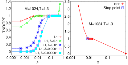
In Fig. 1, using data from a $4XY$ model on Erdos-Renyi (ER)-like sparse graph, we show how the TNR/TPR ratio increases to $1$ as the parameter $\lambda$ used for the $\ell_{1}$-regularization, i.e., ${\cal L}^{(0)}_{i}-\lambda||J||_{1}$, is increased. Further on a $\delta$-threshold criterion Aurell and Ekeberg (2012) is adopted for model selection, i.e., the ability to reduce the number of parameters to the relevant ones. Within the $\delta$-threshold criterion, couplings which are inferred, in absolute value, to be less than $\delta$ are considered to be irrelevant and are set to zero. The value for $\delta$ is, however, chosen a priori and the choice might be delicate when there is not a clear gap in the distribution of the inferred couplings Decelle and Ricci-Tersenghi (2014). Moreover, as $\lambda$ is small, we see that the smaller the $\delta$ the less precise the network reconstruction. On the other hand, the smaller the $\lambda$ the less perturbed the original pseudolikelihood (PL). Indeed, increasing $\lambda$ the chance of globally underestimate the couplings increases.

If the probability distributions of the estimators are known, the issues related to an a priori fixing of a $\delta$ threshold might be overcome through a more accurate hypothesis testing procedure. Indeed, it can be seen that, as $M\rightarrow\infty$, the probability distribution of the maximum PL estimator is a Gaussian with variance given by the diagonal element of the inverse of the Fisher information matrix Wasserman (2003). Therefore, as detailed in Methods, we can construct a confidence interval for each estimated value and verify whether it is compatible with the hypothesis “being a zero coupling”. If it is the case, it is considered as an irrelevant parameter and erased. As we can see from Figs. 1 and 2 this criterion for model selection outperforms, for every value of $\lambda$, the $\delta$-threshold method. Moreover, as detailed in the Methods, this criterion provides a method to determine the best value for the regularizer $\lambda$ that is usually chosen arbitrarily.

Always in Fig. 1 (right) we display the TNR/TPR ratio obtained with the decimation PLM as the fraction of non-decimated couplings $x$ decreases (from fully connected limit $x=1$ to non-interacting graph $x=0$). At $x=1$ the TPR is always one, for any $M$ and $T$, whereas the TNR$=0$. As the fraction of non-decimated couplings decreases but remains greater than or equal to the true one ($x^{*}=2/15$ in the original model analyzed in the right panel of Fig. 1) the TPR does not decrease and the TNR increases towards one. Eventually, more couplings than those of the original network are decimated: the TPR starts decreasing and the ratio TNR/TPR consequently grows above $1$ as $x\to 0$. The blue square indicates the stopping point of the decimation procedure determined, instead, as the maximum of the $\mathcal{L}_{t}$, cf. Eq. (13). It can be observed that in this case it perfectly reconstructs the network of interactions since the TPR=TNR=$1$.

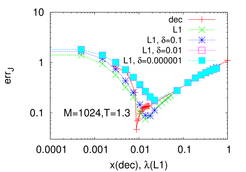
Decimation PLM. When comparing the performances of the most efficient regularization method with the decimation one, we observe that the network reconstruction in terms of true and false couplings is very adequate with both methods. However, the order of magnitude of the reconstruction error, testing also the quality of the inferred values of the couplings, is smaller in the decimation PLM, cf. Fig. 2, when the fraction of decimated couplings ($1-x$) equals the one of the true network. It is important to underline that, within the decimation PLM, no parameters are determined a priori: the optimum value of $x$ is determined maximizing the $\mathcal{L}_{t}$. Moreover, exact fraction of relevant parameters and best estimate of their values are simultaneously inferred, which is not always true in the PLM with $\ell_{1}$-regularization since even the smallest $\lambda$ for network reconstruction might induce a too high global underestimation of the couplings. We, thus, deepen the analysis of the decimation PLM.

Figure 2: Reconstruction error for the $4XY$ model on sparse Erdos-Renyi graph with $N_{q}=N=16$, $M=1024$ at $T=1.3$. The error obtained following various $\ell_{1}$-regularized PLMs is displayed vs. $\lambda$; the decimation PLM reconstruction error is plotted against the fraction of non-decimated couplings $x$.

Figure 3: TPR (Left) and TNR (Right) for decimated networks at the maximum $x^{M}$ of the tilted pseudolikelihood $\mathcal{L}_{t}$ vs $T$ at different data-set sizes $M$ for the $4XY$ model on sparse Mode-Locked graphs with $N=16$, $N_{q}=47$, $T_{c}(N)\simeq 0.50$ ($T_{c}(\infty)=0$).

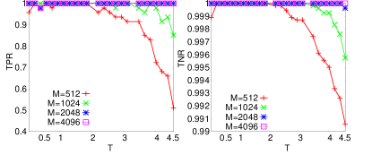
In Fig. 3 we display TPR (left) and TNR (right) vs. $T$ and $M$ for the decimated network at the maximum point, $x^{M}$, of the $\mathcal{L}_{t}$ for the $4XY$ model on a Mode-Locked-like sparse graph with $N_{q}=47$ number of quadruplets and $N=16$ nodes. For large enough $M$ the reconstruction is optimal for all temperatures, whereas for small $M$ it is guaranteed only in a $T$ interval around the finite size proxy to the critical temperature (see Methods). Indeed, we observed that, tuning the external temperature-like parameter for each system studied, one can identify a “critical” $T$ interval where the reconstruction error is minimal, even orders of magnitude smaller than outside such interval, and, more in general, the system is better and easier reconstructed. 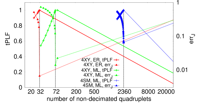In Fig. 4, the behavior of the $\mathcal{L}_{t}$ versus $x$ is compared to err${}_{J}(x)$ for three different systems, the $4XY$-model on ML and ER sparse graphs and the $4$SM-model on a dense ML graph. All systems have $N=32$ variable nodes while the number of interaction quadruplets is $N_{q}=32,72$ and $2360$, respectively. 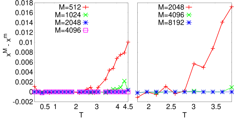The number of configurations in all cases is $M=65000$. It is clearly observed that, given a large enough $M$ and/or a critical-like $T$ the maximum point of the $\mathcal{L}_{t}$, $x^{M}$, coincides with the minimum point of err_J, $x^{m}$. The decimation PLM gives then a criterion to determine the number of interaction couplings in the system from measurements data without any a priori chosen parameters. We notice that, as $M$ is small and $T$ far from the critical region, the maximum point of $\mathcal{L}_{t}$ and minimum point of err_J can be mismatched, as shown in Fig. 5. 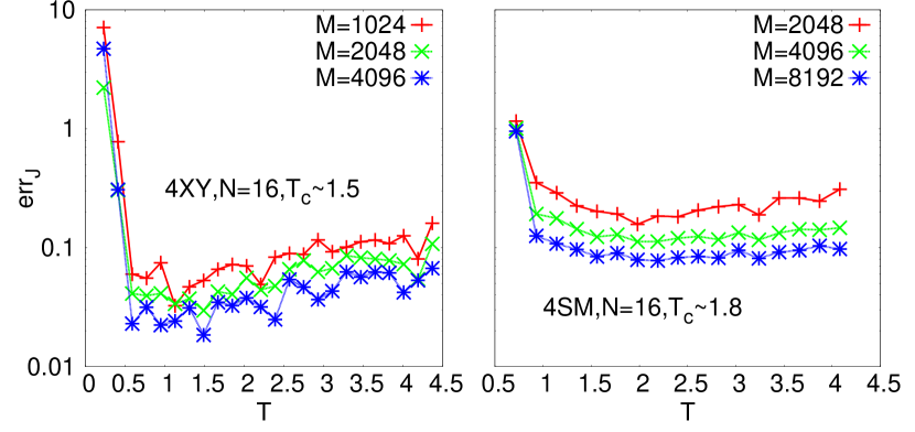In Fig. 6 the $T$ dependence of err_J is plotted for the $4XY$ model on a ER sparse graph and for the $4$SM model on a ML dense graph at different values of $M$. As detailed in Methods the critical $T$ interval turns out to be identified by the (finite size) critical temperature estimate of the phase transition point of the direct statistical mechanical problem.

Figure 4: Tilted pseudolikelihood tPLF (normalized to its maximum) and reconstruction error for different models. Concave curves are tPLF, convex curves are err_J. Three apart models on different random graphs are considered. Red (left) curves: $4XY$ model on sparse Erdos-Renyi graph with $N=32,N_{q}=32$, $M=65000$, at $T=1.2$ ($T_{c}(32)\simeq 1.39$). Green (mid) curves: $4XY$ model on sparse Mode-Locked graph with $N=32,N_{q}=72$, $M=65000$, at $T=1.8$ ($T_{c}(32)\simeq 0.72$). Blue (right) curves: $4$SM model on dense Mode-Locked graph with $N=32,N_{q}=2360$, $M=65000$, at $T=6.2$ ($T_{c}(32)\simeq 0.91$).

Figure 5: Plot of the difference between the maximum point of $\mathcal{L}_{t}$, $x^{\rm M}$, and the minimum point of the reconstruction error, $x^{\rm m}$, vs $T$ at different $M$ for systems of $N=16$ variables. Left: $4$-$XY$ model on sparse Mode-locked graph with $N_{q}=47$ ($T_{c}(16)\simeq 0.50$). Right: $4$SM model on dense Mode-Locked graph with $N_{q}=252$ ($T_{c}\simeq 1.07$).

Figure 6: Reconstruction error at its minimum $x^{\rm min}=x^{\rm true}$ in the decimation procedure vs. $T$ for various $M$ for $N=16$ variables systems with bimodal random values of the coupling constants. Left: $4XY$ model on sparse Erdos-Renyi graph with $N=16,N_{q}=16$. Right: $4$SM model on dense Mode-Locked graph with $N=16,N_{q}=252$.

Discussion
We have been applying and improving Pseudo-Likelihood Maximization(PLM) techniques to the inverse problem in multi-body models, representing systems with nonlinerar response in generic theories. Firstly, we have quantitatively measured the quality of the network reconstruction showing that both PLM methods analyzed allow to obtain an optimal reconstruction for these systems in all thermodynamic phases, when large enough number of samples $M$ are available. Decreasing $M$ the optimal reconstruction is better achieved around the finite size proxy to the critical temperature. Performing then a deeper analysis of the reconstruction error, which gives information on how far the inferred couplings are from the true couplings, reveals that with the decimation PLM the inferred values are closer to those ones of the original systems. Our analysis has been motivated by the study of lasers in the framework of statistical mechanics, though, looking at the models employed, Eqs. (1,Inverse problem for multi-body interaction of nonlinear waves), its range of applicability is more widespread and potentially involves many problems in which both nonlinear and multi-body contributions turn out to be relevant in determining the system behavior, see, e.g., Haus (2000); Wiersma (2008); Mézard et al. (2002); Kay" (2003); Mézard and Montanari (2009); Götze (2009); Katz et al. (2011). Focusing on optics, data from experiments would allow to identify active and passive mode-locking in multimode lasers in terms of mode-coupling coefficients. When more modes on the network graph are connected by a non-vanishing coupling they are matched in frequency, cf. Eq. (3), and therefore, beyond some critical point, they will be locked in phase. Configurations of magnitudes and phases can be obtained from the Fourier analysis of the pulses in ultrafast multimode lasers Kane and Trebino (1993); Trebino et al. (1997); Trebino (2002), pulses known to occur because of mode-locking, and parameters like the self amplitude modulation coefficients of saturable absorbers and the Kerr parameter can be inferred. In presence of relevant light scattering, instead, occurring in random lasers, no direct measurements of phases has been carried out so far, to our knowledge, but only spectral intensities, i.e., modes magnitudes. Acquiring also phases configurations, our inference technique would give the possibility to determine the strength of the interaction among the modes in the systems and to discriminate whether or not self-starting mode-locking occurs in random lasers.

Methods
Data Generation.  Configurations are generated by means of Monte Carlo numerical simulations of the Hamiltonians of the SM, Eq. (1), and the XY, Eq. (Inverse problem for multi-body interaction of nonlinear waves) models with number of modes $N=8,16,32$. In the SM model diluted dense graphs are simulated, i. e., with a total number of quadruplets $N_{q}\sim N^{3}$ and with an average number of couplings per variable $N_{q}/N=O(N^{2})$. We generate graphs of two kinds. One kind is à la Erdos-Renyi: every mode participates in a number of couplings chosen with a Poissonian distribution but independently from each other. The other kind is Mode-Locked: a mode interacts with other three modes only if their frequencies satisfy one of the frequency matching condition permutations, cf. Eq. (3). In the XY model graphs are sparse, i. e., $N_{q}/N=O(1)$ and we generate both models on standard ER graphs and on ML graphs. In order to speed up thermalization and have access to data at equilibrium the Parallel Tempering algorithm has been used. Configuration recording is performed at Monte Carlo steps far enough to avoid data correlation in the critical region.

Maximization algorithm.  In our analysis, rather than maximizing ${\cal L}^{(0)}_{i}({\bm{J}})-\lambda||J||_{1}$ and ${\cal L}(x,{\bm{J}})$, we invert the functional signs and minimize, in order to use well established packages available. For the minimization of -PL with $\ell_{1}$-regularization we adopted L1General Schmidt (2010): a set of MATLAB routines implementing several of the available unconstrained minimization strategies for solving $\ell_{1}$-regularization problems. In particular, the results here presented were obtained with the spectral projected gradient method Schmidt (2010). For the minimization of $-{\cal L}(x,{\bm{J}})$ in the decimation procedure, we use, instead, Open Optimization Library (OOL) Biloti et al. (2005), which is a set of constrained optimization codes written in C. The results here presented were obtained using the spectral projected gradient method for convex set Birgin et al. (2000). The decimation code using the OOL routine has been ad hoc developed with parallel programming on GPU’s, reducing the running times of numerical processing with respect to C++ codes on CPU up to a factor $5$ for the largest analyzed systems, $N=32$. In terms of timing, the parallel CUDA code outperforms the MATLAB routines up to a factor $30$ for $N=16$.

Inverse algorithm To evaluate the inverse of the Fisher Information matrix, defined by

$$\mathcal{I}^{i}_{ab}=-\frac{\partial^{2}\mathcal{L}_{i}}{\partial J_{a}\partial J_{b}}\bigg{|}_{\hat{\mathbf{J}}}$$ (14)

where with $a$, $b$ we indicate two possible quadruplets node $i$ might belong to (see next paragraph), we first evaluate its Cholesky decomposition, being $\mathcal{I}^{i}_{ab}$ a symmetric, positive define square matrix, and then its inverse through GSL libraries.
Pseudolikelihood function From Eq. (1) in the main text, the likelihood function of a mode amplitude configuration $\bm{a}$, given a coupling set ${\bm{J}}$, is readily introduced as

$$P(\bm{a}|\bm{J})=\frac{1}{Z[\bm{J}]}\exp\left\{-\beta{\cal H}[\bm{a}|\bm{J}]\right\}$$

To construct the likelihood function of $a_{j}$, i. e., the probability distribution of a single variable given the values of all the other variables $\bm{a}_{\backslash j}$, we first rewrite Eq. (1) in an equivalent way:

$${\cal H}[\bm{a}|\bm{J}] = -\frac{1}{8}\sum_{j=1}^{N}a_{j}H_{j}[\bm{a}_{\backslash j},\bm{J}]+\mbox{c.c.}$$

defining the complex-valued local effective fields

$$H_{j}[\bm{a}_{\backslash j},\bm{J}] = \frac{1}{4}\sum^{\rm d.i.}_{klm\neq j}J_{jklm}{\cal F}_{klm}$$

$${\cal F}_{klm} = \frac{1}{3}\left[a_{k}^{*}a_{l}a_{m}^{*}+a_{k}a_{l}^{*}a_{m}^{*}+a_{k}^{*}a_{l}^{*}a_{m}\right]$$

Then, we separate the contributions from a given variable $a_{i}$ from all contributions not involving $a_{i}$, only $\bm{a}_{\backslash i}$:

$${\cal H}[\bm{a}|\bm{J}] = -\frac{1}{8}a_{i}H_{i}[\bm{a}_{\backslash i},\bm{J}]$$ (15)

$$-\frac{1}{8}\sum_{j\neq i}^{1,N}a_{j}H_{j}[\bm{a}_{\backslash j},\bm{J}]+\mbox{c.c.}$$

$$= {\cal H}_{i}[a_{i}|\bm{a}_{\backslash i},\bm{J}]+{\cal H}_{\backslash i}[\bm{a}_{\backslash i}|\bm{J}]$$

In terms of this decoupling the partition function reads:

$$Z = \sum_{\bm{a}_{\backslash i}}\exp\left\{-\beta{\cal H}_{\backslash i}[\bm{a}_{\backslash i}|\bm{J}]\right\}Z_{i}[{\bm{a}_{\backslash i}},\bm{J}]$$ (16)

with

$$Z_{i}[{\bm{a}_{\backslash i}}]\equiv\sum_{a_{i}}\exp\left\{a_{i}H_{i}[\bm{a}_{\backslash i},\bm{J}]+\mbox{c.c.}\right\},$$

i. e., Eq. (9) of the main text. In order to effectively carry out the sum over $a_{i}$ values one has to recall that the phasors satisfy a global spherical constraint $\sum_{j}|a_{j}|^{2}=\epsilon N$, with constant $\epsilon$. Once all $\bm{a}_{\backslash i}$ are given, then, the value of $|a_{i}|$ is fixed,

$$|a_{i}|=\sqrt{\epsilon N-\sum_{j\backslash i}|a_{j}|^{2}}$$

and $\sum_{a_{i}}$ simply reduces to an integral on the angular phase variable $\phi_{i}\in[0:2\pi[$. Using Eqs. (15) and (16) of this section the pseudolikelihood function of the values of $a_{i}$, biased by $\bm{a}_{\backslash i}$ values, can be, eventually, written as

$$P_{i}(a_{i}|\bm{a}_{\backslash i},\bm{J}) = \frac{1}{Z_{i}[\bm{a}_{\backslash i},\bm{J}]}\exp\left\{a_{i}H_{i}[\bm{a}_{\backslash i},\bm{J}]+\mbox{c.c.}\right\}$$

In order to find the best estimates of the interaction parameters given a data set of $M$ mode amplitude configurations, we minimize the opposite log-pseudolikelihood functional $-{\cal L}_{i}$:

$$-{\cal L}_{i} = -\sum_{\mu=1}^{M}\left(a_{i}^{\mu}H_{i}[\bm{a}_{\backslash i}^{\mu},\bm{J}]+\mbox{c.c.}\right)+\sum_{\mu=1}^{M}\ln Z_{i}[\bm{a}^{\mu}_{\backslash i},\bm{J}]$$

with respect to the coupling parameters, exploiting the explicit knowledge of the derivatives

$$\frac{\partial(-{\cal L}_{i})}{\partial J_{ijkl}}=\sum_{\mu=1}^{M}{\cal F}^{\mu}_{jkl}\left[\langle a_{i}\rangle_{i}^{\mu}-a_{i}^{\mu}\right]$$ (18)

where we denoted

$$\langle\left(\ldots\right)\rangle_{i}\equiv\frac{1}{Z_{i}[\bm{a}^{\mu}_{\backslash i},\bm{J}]}\sum_{a_{i}}\left(\ldots\right)\exp\left\{a_{i}H_{i}[\bm{a}_{\backslash i}^{\mu},\bm{J}]+\mbox{c.c.}\right\}.$$

Rewriting the complex amplitude in polar coordinates $a_{i}=A_{i}e^{\imath\phi_{i}}$ we have the following expression for the marginal (we do not write the $\bm{J}$ dependence)

$$P_{i}(A_{i},\phi_{i}|\bm{A}_{\backslash i},\bm{\phi}_{\backslash i}) = \frac{\exp\left\{A_{i}\left[H_{i}^{R}~{}\cos\phi_{i}+H_{i}^{I}~{}\sin\phi_{i}\right]\right\}}{Z_{i}[\bm{A}_{\backslash i},\bm{\phi}_{\backslash i}]}$$ (19)

$$= \frac{\exp\left\{A_{i}|H_{i}|\cos(\phi_{i}-\gamma_{i})\right\}}{2\pi\int dA_{i}~{}I_{0}(A_{i}|H_{i}|)}$$

where

$$|H_{i}| = \sqrt{\bigl{(}H_{i}^{R}\bigr{)}^{2}+\bigl{(}H_{i}^{I}\bigr{)}^{2}}$$

$$\gamma_{i} = \arctan\frac{H_{i}^{I}}{H_{i}^{R}}$$

and $I_{0}(x)$ is the modified Bessel function of the first kind.

As mentioned in the main text, the polar coordinates are most useful in the cases of intensity equidistribution among the modes, $A_{i}\simeq 1$, $\forall~{}i$, and of quenched amplitudes, i.e., when the $A_{i}$ dynamics is quenched on the time scales of the $\phi$’s dynamics. In the latter case all $A$’s are taken care of by rescaling the coupling constants as $A_{i}A_{j}A_{k}A_{l}J_{ijkl}\to J_{ijkl}$. When the couplings are considered real-valued, the polar expressions of the local effective fields, cf. Eq. (7) in the main text, can be rewritten by substituting Eq. (8) with

$${\cal F}^{R}_{jkl} = \cos\phi_{j}\cos\phi_{k}\cos\phi_{l}+\frac{1}{3}(\cos\phi_{j}\sin\phi_{l}\sin\phi_{k}$$

$$+ \cos\phi_{l}\sin\phi_{j}\sin\phi_{k}+\cos\phi_{k}\sin\phi_{j}\sin\phi_{l})\quad$$

$${\cal F}^{I}_{jkl} = \sin\phi_{j}\sin\phi_{k}\sin\phi_{l}+\frac{1}{3}(\sin\phi_{j}\cos\phi_{l}\cos\phi_{k}$$

$$+ \sin\phi_{l}\cos\phi_{j}\cos\phi_{k}+\sin\phi_{k}\cos\phi_{j}\cos\phi_{l})\quad$$

and the log-pseudolikelihood functional ${\cal L}_{i}$ and its gradient, cf. Eqs. (LABEL:eq:pl_4a_APP,18) in this section, simplify to

$$-{\cal L}_{i} = \sum_{\mu=1}^{M}\Biggl{\{}\ln 2\pi I_{0}\left(\left|H_{i}(\bm{\phi}_{\backslash i}^{\mu})\right|\right)$$

$$-\Bigl{[}H^{R}_{i}(\bm{\phi}_{\backslash i}^{\mu})\cos\phi_{i}^{\mu}+H_{i}^{I}(\bm{\phi}_{\backslash i}^{\mu})\sin\phi_{i}^{\mu}\Bigr{]}\Biggr{\}}$$

$$\frac{\partial(-{\cal L}_{i})}{\partial J_{ijkl}} = \sum_{\mu=1}^{M}\Biggl{\{}{\cal F}_{jkl}^{\mu}$$

$$\times\left[\frac{I_{1}(|H_{i}(\bm{\phi}_{\backslash i}^{\mu})|)}{I_{0}(|H_{i}(\bm{\phi}_{\backslash i}^{\mu})|)}\frac{H_{i}(\bm{\phi}_{\backslash i}^{\mu})}{|H_{i}(\bm{\phi}_{\backslash i}^{\mu})|}-e^{\imath\phi_{i}^{\mu}}\right]+\mbox{c.c.}\Biggr{\}}$$

To determine the interaction network of non-linear wave systems we use and compare two techniques: the $\ell_{1}$-regularization PLM Ravikumar et al. (2010); Aurell and Ekeberg (2012) and the decimation PLM Decelle and Ricci-Tersenghi (2014).
$\ell_{1}$-regularization In this approach we add a $\ell_{1}$ norm contribution for each coupling to be inferred to the log-pseudolikelihood in order to keep the coupling values from diverging during the minimization procedure:

$$-{\cal L}_{i}\to-{\cal L}_{i}+\lambda\sum_{jklm}^{\rm d.i.}|J_{jklm}|$$ (21)

The positive regularizer $\lambda$ must be small in order to prevent the modification of the landscape of ${\cal L}_{i}$. We take a pseudolikelihood that is intensive in $M$ but small enough values of $\lambda$ for all $M$’s.

Within this method, for each mode $i$ all couplings involving $i$ are inferred in one apart iteration. The same quadruplet $J_{ijkl}$ can, thus, be inferred more times, proceeding by minimizing likelihood functions for different, though interacting, modes $i$, $j$, $k$ and $l$. Nothing prevents the values of apart reconstructions to be the same. Eventually, thus, all inferred values of the same coupling are averaged in order to enforce the original symmetry.
$\delta$ thresholding A further improvement in the reconstruction of the topology can be achieved, as suggested in Ref. Aurell and Ekeberg (2012), by setting to zero all couplings whose estimate is below a threshold value $\delta$. However, the choice of the $\delta$ value might be delicate since there are many cases in which there is no clear gap between the zero and the non-zero couplings Decelle and Ricci-Tersenghi (2014). If the probability distributions of the estimators are known, we can overcome this problem developing a more accurate hypothesis testing scheme.
$\mathcal{P}(\hat{J})$ thresholding It can be seen that, as $M\rightarrow\infty$, the probability distribution $\mathcal{P}(\hat{J})$ of the maximum PL estimator $\hat{J}$ converges to a Gaussian distribution centered around the true value of the coupling and with variance estimated by the diagonal elements of the inverse of the Fisher information matrix Wasserman (2003). The elements, $\mathcal{I}^{i}_{ab}$, of the Fisher information matrix are defined through:

$$\mathcal{I}^{i}_{ab}=-\frac{\partial^{2}\mathcal{L}_{i}}{\partial J_{a}\partial J_{b}}\bigg{|}_{\hat{\mathbf{J}}}$$

where with $a$, $b$ we indicate two possible quadruplets including node $i$, i.e., $a=\{i,j,k,l\}$, $b=\{i,j^{\prime},k^{\prime},l^{\prime}\}$. Then, knowing the distribution, we can determine, for every estimated value $J^{*}_{a}$, if it is compatible with a Gaussian centered in zero, i.e., if the hypothesis for the true coupling to be zero might or not be rejected.

The hypothesis testing can be schematically developed as follows.

1. Once the maximum points of the PL are found, we evaluate the inverse of the Fisher information matrix, Eq. (Inverse problem for multi-body interaction of nonlinear waves); from Eq. (Inverse problem for multi-body interaction of nonlinear waves), we have:

   $$\mathcal{I}^{i}_{ab} = \sum_{\mu=1}^{M}\mathcal{F}^{\mu}_{a}\mathcal{F}^{\mu}_{b}\Biggl{\{}$$

   $$\times\biggl{(}\frac{H_{i}(\bm{\phi}_{\backslash i}^{\mu})}{\left|H_{i}(\bm{\phi}_{\backslash i}^{\mu})\right|}\biggl{)}^{2}\mathcal{B}\left(\left|H_{i}(\bm{\phi}_{\backslash i}^{\mu})\right|\right)$$

   $$+\frac{I_{1}(|H_{i}(\bm{\phi}_{\backslash i}^{\mu})|)}{I_{0}(|H_{i}(\bm{\phi}_{\backslash i}^{\mu})|)}\biggl{(}\frac{\left|H_{i}(\bm{\phi}_{\backslash i}^{\mu})\right|^{2}-\left(H_{i}(\bm{\phi}_{\backslash i}^{\mu})\right)^{2}}{\left|H_{i}(\bm{\phi}_{\backslash i}^{\mu})\right|^{3}}\biggr{)}\Biggr{\}}$$

   where with $\mathcal{B}\left(x\right)$ we indicate:

   $$\mathcal{B}\left(x\right)=\frac{1}{2}\left(\frac{I_{2}(x)}{I_{0}(x)}+1\right)-\left(\frac{I_{1}(x)}{I_{0}(x)}\right)^{2}$$

   The diagonal terms of the inverse matrix are taken as estimates for the variances, $\sigma^{*}_{a}$, of the estimator distributions.

2. We assume every couplings to be zero; hence, we expect every estimated value $J^{*}_{a}$ to be compatible with $N\left(0,\sigma^{*}_{a}\right)$ distribution. We, then, construct a confidence interval $C_{n}$ that should contain the estimated value $J^{*}_{a}$ within a $97.5\%$ probability.

3. If the inferred $J^{*}_{a}$ is contained in $C_{n}$ we accept the zero hypothesis and the coupling is set to zero.

Optimal $\lambda$ regularizer It is clear from Eq. (21), that as $\lambda$ increases it increases the tendency to globally underestimate the interaction couplings. Within the hypothesis testing procedure described more and more couplings become compatible with a Gaussian centered in zero and are considered as irrelevant. Indeed, as noticed in Fig. 1, $\mbox{err}_{J}(\lambda)$ increases above some optimal value $\hat{\lambda}$ that should depend on the number of configurations $M$ available and on $T$. One procedure that might be adopted to determine $\hat{\lambda}$ consists in testing the PLM with $\ell_{1}$-regularization on data relative to a known system and use the optimum value found to solve the inverse problem of new systems. However, there might be cases in which there are no solved inverse problems available and, in general, $\hat{\lambda}$ could depend on the details of the problem.
The hypothesis testing procedure explained in the previous paragraph could be considered also as a tool to determine $\hat{\lambda}$. Indeed, within the PLM, every coupling $J_{ijkl}$ has four estimators $J^{*}_{a}$ and we evaluate the $\sigma^{*}_{a}$ for each one. It might be that not all the four estimated values have the same compatibility with a Gaussian centered in zero since, due to the lack of configurations, one value might be overestimated. Increasing $\lambda$, the number of quadruplets for which the hypothesis test does not give the same answer for every estimated value decreases. We observed that the minimum $\lambda$ value for which there are no quadruplets that answer differently to the hypothesis test is very close, within less than an $8\%$ difference, to $\hat{\lambda}$.
PLM Decimation In the decimation procedure we maximize the total log-likelihood for all modes

$${\cal L}\equiv\frac{1}{N}\sum_{i}^{N}{\cal L}^{(0)}_{i}$$ (23)

starting from ${\cal L}_{\rm max}$ defined on a full graph and inferring all the values of the $N_{q}=N(N-1)(N-2)(N-3)/24\sim N^{4}$ couplings on that network. Sorting the couplings by their absolute value and taking away (decimating) the $N_{0}$ smallest we are left with a network of $N_{q}-N_{0}=xN_{q}$ non-zero couplings. A new inference iteration, including minimization of ${\cal L}(x)$ and sorting, will allow to decimate further another group of the smallest couplings. And so on and so forth, as far as the couplings of the decimated model network are more than the couplings of the true system. Indeed, as far as the number of inferred parameters is larger than the true number of parameters the pseudolikelihood is not expected to change and will stick to its maximum value ${\cal L}_{\rm max}$ (overfitting). The indication of the true number of couplings will be given, indeed, right by the $x$ value of the fraction of non-decimated couplings across which ${\cal L}$ starts decreasing because the number of inferred parameters is less than the real number of parameters (underfitting). The minimum conceivable ${\cal L}(x)$ is for the non-interacting system: ${\cal L}_{\rm min}={\cal L}(0)$. To enhance the determination of the true network connectivity $x^{*}$, below which statistical interpolation becomes less reliable, Decelle and Ricci-Tersenghi Decelle and Ricci-Tersenghi (2014) introduced the tilted pseudolikelihood ${\cal L}_{t}$

$${\cal L}_{t}\equiv{\cal L}(x)-x{\cal L}_{\rm max}-(1-x){\cal L}_{\rm min}$$

such that

$${\cal L}_{t}(0)={\cal L}_{t}(1)=0$$

$${\cal L}_{t}(x\leq x^{*})\simeq x({\cal L}_{\rm max}-{\cal L}_{\rm min}).$$

We stress that using the total likelihood, cf. Eq. (11), the symmetry of coupling constants under indices permutation is automatically enforced.
Random Graphs We report the distributions of connectivities in the various graphs that we used to test the reconstruction methods exposed in the main manuscript for the complex spherical model (SM), cf. Eq. (1), and the XY model, cf. Eq. (Inverse problem for multi-body interaction of nonlinear waves), at finite $N$. In the XY models the $x$ axis is the connectivity per variable. In the SM the total number of couplings scales like $N^{3}$: the $x$ axis represents, in this case, the connectivity per variable node rescaled by $N^{2}$.

$N$	phasor ER	phasor ML	XY ER	XY ML
$16$	$N_{q}=366$	$N_{q}=252$	$N_{q}=16$	$N_{q}=47$
$32$	$N_{q}=2949$	$N_{q}=2360$	$N_{q}=32$	$N_{q}=72$
$128$	$N_{q}=188742$	$N_{q}=168672$	$N_{q}=128$	$N_{q}=275$

Table 1: Total number of quadruplets in all simulated networks used to yield data to be tested by our pseudolikelihood inference methods.

Figure 7: Distribution of connectivity per variable node of the $4$XY models on ER-like (left) and Mode-Locking-like (right) sparse graphs of sizes $N=16,32,128$. The blue curves in the right panels are Poisson distributions with same mean as the empirical distributions.

Figure 8: Distribution of rescaled connectivity $c/N^{2}$ in the $4$-phasor models - termed "spherical model" (SM) in the plots - on ER-like and ML-like dense ($O(N^{3})$) graphs of sizes $N=16,32,128$. The blue curves in the right panels are Poisson distributions with same mean as the data derived distributions.

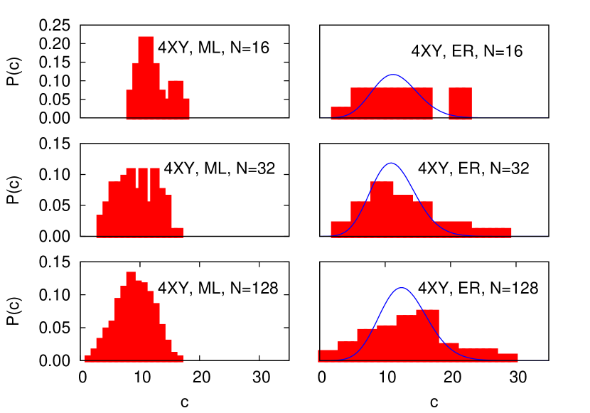
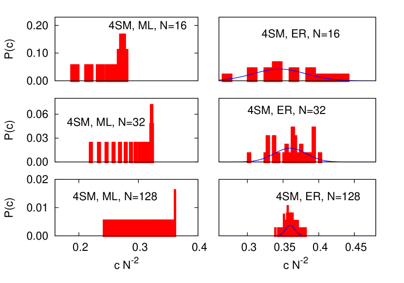
The distributions in the Erdos-Renyi-like graphs and in the Mode-Locked-like graphs in pairwise interacing systems are known to tend to Poissonian distributions in the thermodynamic limiti $N\to\infty$ Marruzzo (2016), though the ML-graph convergence is much slower for increasing $N$. As a comparison, in the right panels of Figs. 7, 8 we plot the relative Poissonian distributions with the same average. Finite size effects are clearly strong for the small simulated sizes. The actual number of quadruplet couplings $N_{q}$ for each simulated instance is reported for all considered models in Tab. 1.
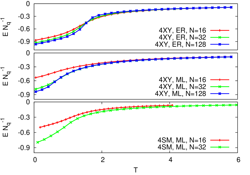
Finite size critical temperature We refer several times to a critical region in $T$ for which inference works better that at higher or lower $T$. In particular, the reconstruction error is up to one order of magnitude smaller and the network topology is correctly reconstructed with the need of less configurations data. In Fig. 9 we display the energy plots of the models used to produce equilibrium data with Exchange Monte Carlo simulations. In the thermodynamic limit $N\to\infty$ they should display a true critical point behavior where a phase transition occurs from a paramagnetic-like phase to a phase-locked or to a spin-glass phase. For the $4$XY model on ER sparse graphs these temperatures are analytically known, as $T_{c}=0$ for $N_{q}/N=1$ and $T_{c}>0$ for $N_{q}/N=2$ Marruzzo and Leuzzi (2016). For finite sizes the mathematical discontinuity is approximated by a steep, though smeared, descent as $T$ decreases. This step becomes steeper and steeper as $N$ increases, eventually reaching the limit of a true singularity representing a true phase transition. Indeed, for finite systems, no actual phase transition occurs. However, one can identify finite size pseudocritical points that, for systems of increasing size $N$, form a series converging to the true critical point. Operatively, we take as finite size critical points $T_{c}(N)$ the peak of the specific heat $dE/dT$ from $E_{N}(T)$ data in Fig. 9. For the simulated systems whose energy is displayed in Fig. 9 the $T_{c}(N)$ are reported in Tab. 2.

Figure 9: Internal energy vs. temperature in various simulated instances of the models of Eqs. (1,Inverse problem for multi-body interaction of nonlinear waves)

$N$	phasor ML	XY ER	XY ML
$16$	$1.07(1)$	$1.34(1)$	$0.50(1)$
$32$	$0.91(1)$	$1.39(1)$	$0.72(1)$
$128$		$1.53(1)$	$0.63(1)$

Table 2: Finite size proxies for the critical point.

Authors Contributions A.M., P.T., F.A., A.P. and L.L. work on the programs solving the inverse problems and on the data analysis as well as on the Monte Carlo simulations and on the graphs analysis. A.M., P.T., F.A., A.P. and L.L. reviewed and approved the final version of this manuscript.
Additional Information
Competing financial interests The authors declare no competing financial interests.
Acknowledgements
We thank Federico Ricci Tersenghi for fruitful discussions. This project has received funding from the European Research Council (ERC) under the European Union’s Horizon 2020 research and innovation program, Project LoTGlasSy, Grant Agreement No. 694925 and from the Italian Ministry for Education, University and Research (MIUR) under the PRIN 2015, Project Statistical Mechanics and Complexity, CINECA code 2015K7KK8L_005.

References

- Sargent III et al. (1978) M. Sargent III, M. O’Scully, and W. E. Lamb, Laser Physics (Addison Wesley Publishing Company, 1978).
- Haus (2000) H. A. Haus, IEEE J. Quantum Electron. 6, 1173 (2000).
- Gordon and Fischer (2002) A. Gordon and B. Fischer, Phys. Rev. Lett. 89, 103901 (2002).
- Katz et al. (2006) M. Katz, A. Gordon, O. Gat, and B. Fischer, Phys. Rev. Lett. 97, 113902 (2006).
- Antenucci et al. (2015a) F. Antenucci, M. Ibáñez Berganza, and L. Leuzzi, Phys. Rev. A 91, 043811 (2015a).
- Antenucci et al. (2015b) F. Antenucci, M. Ibañez Berganza, and L. Leuzzi, Phys. Rev. B 92, 014204 (2015b).
- Lawandy et al. (1994) N. M. Lawandy, R. M. Balachandran, A. S. L. Gomes, and E. Sauvain, Nature 368, 436 (1994).
- Cao et al. (1998) H. Cao, Y. G. Zhao, H. C. Ong, S. T. Ho, et al., Appl. Phys. Lett. 73, 3656 (1998).
- Wiersma (2008) D. S. Wiersma, Nature Physics 4, 359 (2008).
- Antenucci et al. (2015c) F. Antenucci, C. Conti, A. Crisanti, and L. Leuzzi, Phys. Rev. Lett. 114, 043901 (2015c).
- Monasson and Zecchina (1997) R. Monasson and R. Zecchina, Phys. Rev. E 56, 1357 (1997).
- Mézard et al. (2002) M. Mézard, G. Parisi, and R. Zecchina, Science 297, 812 (2002).
- Kay" (2003) D. J. C. M. Kay", Information Theory, Inference, and Learning Algorithms (Cambridge University Press (Cambridge, UK), 2003).
- Mézard and Montanari (2009) M. Mézard and A. Montanari, Information, Physics, and Computation (Oxford University Press, 2009).
- Kirkpatrick et al. (1989) T. R. Kirkpatrick, D. Thirumalai, and P. G. Wolynes, Phys. Rev. A 40, 1045 (1989).
- Crisanti and Sommers (1992) A. Crisanti and H. Sommers, Z. Phys. B 87, 341 (1992).
- Götze (2009) W. Götze, Complex Dynamics of Glass-Forming Liquids: A Mode-Coupling Theory (Oxford University Press (Oxord, UK), 2009).
- Franz et al. (2011) S. Franz, G. Parisi, F. Ricci-Tersenghi, and T. Rizzo, The European Physical Journal E 34, 1 (2011).
- Caltagirone et al. (2012) F. Caltagirone, U. Ferrari, L. Leuzzi, G. Parisi, et al., Phys. Rev. Lett. 108, 085702 (2012).
- Ferrari et al. (2012) U. Ferrari, L. Leuzzi, G. Parisi, and T. Rizzo, Phys. Rev. B 86, 014204 (2012).
- Katz et al. (2011) Y. Katz, K. Tunstrom, C. C. Ioannou, C. Huepe, et al., Proc. Nat. Acad. Sci. USA 108, 18720 (2011).
- Herbert-Read et al. (2011) J. E. Herbert-Read, A. Pernab, R. P. Mann, T. M. Schaerf, et al., Proc. Nat. Acad. Sci. USA 108, 18726 (2011).
- Barber (2012) D. Barber, Bayesian Reasoning and Machine Learning (Cambridge University Press (Cambridge, UK), 2012).
- Ravikumar et al. (2010) P. Ravikumar, M. J. Wainwright, and J. D. Lafferty, Ann. Statist. 38, 1287 (2010).
- Aurell and Ekeberg (2012) E. Aurell and M. Ekeberg, Phys. Rev. Lett. 108, 090201 (2012).
- Wasserman (2003) L. Wasserman, All of Statistics: A concise course in statistical inference (Springer, New York, 2003).
- Decelle and Ricci-Tersenghi (2014) A. Decelle and F. Ricci-Tersenghi, Phys. Rev. Lett. 112, 070603 (2014).
- Note (1) This is a diluted dense graph: not all quadruplets are present, though their number per variable node scales with , unlike in sparse graphs. A complete dense graph would contain interacting quadruplets.
- Kuramoto (1975) Y. Kuramoto, Lect. N. Phys. 39, 420 (1975).
- Antoni and Ruffo (1995) M. Antoni and S. Ruffo, Phys. Rev. E 52, 2361 (1995).
- Acebrón et al. (2005) J. A. Acebrón, L. L. Bonilla, C. J. Pérez Vicente, F. Ritort, et al., Rev. Mod. Phys. 77, 137 (2005).
- Gupta et al. (2014) S. Gupta, A. Campa, and S. Ruffo, J. Stat. Mech. , R08001 (2014).
- Fermi et al. (1955) E. Fermi, J. Pasta, and S. M. Ulam, LANL Report. 1940 (1955).
- Ortiz et al. (2013) G. Ortiz, E. Cobenera, and Z. Nussinov, in 40 Years of Berezinskii-Kosterlitz-Thouless Theory, edited by J. V. José (World Scientific Publisher, Singapore, 2013) Chap. 3, pp. 93–134.
- Marruzzo and Leuzzi (2015) A. Marruzzo and L. Leuzzi, Phys. Rev. B 91, 054201 (2015).
- Potts (1952) R. Potts, Proc. Camb. Phil. Soc. 48, 106 (1952).
- Antenucci et al. (2015d) F. Antenucci, A. Crisanti, and L. Leuzzi, Phys. Rev. A 91, 053816 (2015d).
- Boyd (2002) R. W. Boyd, Nonlinear Optics, 2nd ed. (Academic Press, New York, 2002).
- Gordon and Fischer (2003) A. Gordon and B. Fischer, Opt. Comm. 223, 151 (2003).
- Weill et al. (2005) R. Weill, A. Rosen, A. Gordon, O. Gat, et al., Phys. Rev. Lett. 95, 013903 (2005).
- Weill et al. (2010) R. Weill, B. Fischer, and O. Gat, Phys. Rev. Lett. 104, 173901 (2010).
- Angelani et al. (2006) L. Angelani, C. Conti, G. Ruocco, and F. Zamponi, Phys. Rev. B 74, 104207 (2006).
- Leuzzi et al. (2009) L. Leuzzi, C. Conti, V. Folli, L. Angelani, et al., Phys. Rev. Lett. 102, 083901 (2009).
- Svelto (1998) O. Svelto, Principles of lasers (Springer, 1998).
- Note (2) Indeed, it can be seen that for bond-disordered SM’s, if the node connectivity does not increase at least with with , all the power condensates into one single quadruplet below threshold Antenucci et al. (2015b).
- Hugi et al. (2012) A. Hugi, G. Villares, S. Blaser, H. C. Liu, et al., Nature 492, 229 (2012).
- Antenucci et al. (2015e) F. Antenucci, A. Crisanti, and L. Leuzzi, Scientific Reports 5, 16792 (2015e).
- Marruzzo and Leuzzi (2016) A. Marruzzo and L. Leuzzi, Phys. Rev. B 93, 094206 (2016).
- Ghofraniha et al. (2014) N. Ghofraniha, I. Viola, F. Di Maria, G. Barbarella, et al., Nat. Commun. 6, 6058 (2014).
- Gomes et al. (2015) A. S. L. Gomes, E. P. Raposo, A. L. Moura, S. I. Fewo, et al., arXiv:1509.00276 (2015).
- Pincheira et al. (2015) P. I. R. Pincheira, A. F. Silva, S. J. M. Carreno, S. I. Fewo, et al., arXiv:1511.03087 (2015).
- El-Dardiry et al. (2010) R. G. S. El-Dardiry, A. P. Mosk, O. L. Muskens, and A. Lagendijk, Phys. Rev. A 81, 043830 (2010).
- Payal Tyagi, Alessia Marruzzo, Andrea Pagnani, Fabrizio Antenucci, and others (2016) Payal Tyagi, Alessia Marruzzo, Andrea Pagnani, Fabrizio Antenucci, and others, Phys. Rev. B 94, 024203 (2016).
- Kane and Trebino (1993) D. J. Kane and R. Trebino, Opt. Lett. 18, 823 (1993).
- Trebino et al. (1997) R. Trebino, K. W. DeLong, D. N. Fittinghoff, J. N. Sweetser, et al., Rev. Sci. Instr. 68, 3277 (1997).
- Trebino (2002) R. Trebino, Frequency-Resolved Optical Gating: The Measurement of Ultrashort Laser Pulses. (Springer, 2002).
- Schmidt (2010) M. Schmidt, Graphical Model Structure Learning with L1-Regularization, Ph.D. thesis, University of British Columbia (2010).
- Biloti et al. (2005) R. Biloti, L. D’Afonseca, and S. Ventura, “Open optimization library,” (2005).
- Birgin et al. (2000) E. G. Birgin, J. M. Martínez, and M. Raydan, SIAM Journal on Optimization 10, 1196 (2000), http://dx.doi.org/10.1137/S1052623497330963 .
- Marruzzo (2016) A. Marruzzo, Statistical Mechanics of continuous spin models and applications to nonlinear optics in disordered media, PhD Thesis (Sapienza University of Rome, 2016).
Authors Contributions
A.M., P.T., F.A., A.P. and L.L. work on the programs solving the inverse problems and on the data analysis as well as on the Monte Carlo simulations and on the graphs analysis. A.M., P.T., F.A., A.P. and L.L. reviewed and approved the final version of this manuscript.