Fine-To-Coarse Global Registration of RGB-D Scans
Abstract
RGB-D scanning of indoor environments is important for many applications, including real estate, interior design, and virtual reality. However, it is still challenging to register RGB-D images from a hand-held camera over a long video sequence into a globally consistent 3D model. Current methods often can lose tracking or drift and thus fail to reconstruct salient structures in large environments (e.g., parallel walls in different rooms). To address this problem, we propose a “fine-to-coarse” global registration algorithm that leverages robust registrations at finer scales to seed detection and enforcement of new correspondence and structural constraints at coarser scales. To test global registration algorithms, we provide a benchmark with 10,401 manually-clicked point correspondences in 25 scenes from the SUN3D dataset. During experiments with this benchmark, we find that our fine-to-coarse algorithm registers long RGB-D sequences better than previous methods.
1 Introduction
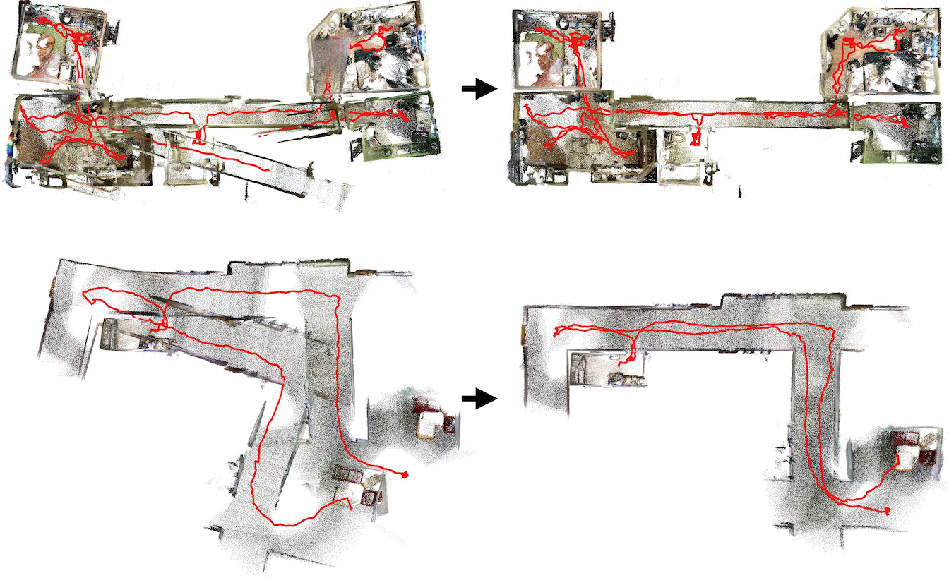
The proliferation of inexpensive RGB-D video cameras allows for easy scanning of static indoor environments, enabling applications in many domains, including cultural heritage, real estate and virtual reality. Motivated by these applications, our goal is to create a method that takes a sequence of RGB-D images captured with a hand-held camera as input and produces a globally consistent 3D model as output. We would like the algorithm to register images robustly in a wide range of indoor environments (offices, homes, museums, etc.), execute off-line within practical computational limits, and work with data acquired by inexpensive commodity cameras, so that it can be used by non-experts.
Despite much prior work, it is still difficult to register RGB-D data acquired with a hand-held camera. Although camera poses can usually be tracked over short distances [28], local tracking often fails in texture-less regions and/or drifts over long ranges [9, 30] (left side of Figure 1). These errors can be fixed with asynchronous or global optimizations based on detected loop closures [8, 19, 46]. However, finding loop closures is difficult without prior constraints in large real-world scans with multiple rooms and/or repeated structures. In our experience, even state-of-the-art global registration methods produce warped surfaces and improbable structures in these cases [8].
To address this issue, global refinement methods have been proposed based on fitting structural models [24, 25, 27] and/or aligning closest point correspondences [5, 14]. However, these methods only succeed when the alignments provided as input are nearly correct. Otherwise, they may detect and amplify erroneous constraints found in the misaligned inputs.
We introduce a new “fine-to-coarse” global registration algorithm that refines an initial set of camera poses by iteratively detecting and enforcing geometric constraints within gradually growing subsets of the scanned trajectory. During each iteration, closest points and geometric constraints (plane parallelism, perpendicularity, etc.) are detected and enforced only within overlapping “windows” of sequential RGB-D frames. The windows start small, such that relative initial alignments are likely to be correct (Figure 2). As the algorithm proceeds, the windows gradually increase in size, enabling detection of longer-range correspondences and large-scale geometric structures leveraging the improved trajectory provided by previous iterations. This process is continued until final window includes the entire scan and a global refinement can be done robustly.

The advantage of this fine-to-coarse approach is that closest point correspondences and planar structures are detected in each iteration only at the scales at which previous iterations have already aligned the scans. Enforcing these constraints in one iteration improves the registration for the next. For example in Figure 3, note how geometric constraints between walls become easier to detect in each iteration (left to right), and enforcement of those constraints gradually rectifies the reconstruction. In the final iteration, the alignment is almost perfect, making it trivial to detect very large-scale structures and long-range constraints (e.g., parallel walls in different rooms), which are crucial for correct global registration.
To evaluate this algorithm and enable comparisons between future algorithms, we have created a new registration benchmark based on the SUN3D dataset [47]. It contains 10,401 manually-clicked point correspondences in RGB-D scans containing 149011 frames in 25 scenes, many of which span multiple rooms. During experiments with this new benchmark, we find that our fine-to-coarse algorithm produces more accurate global registrations and handles more difficult inputs than previous approaches.
Overall, the research contributions of this paper are three-fold. First, we propose a new fine-to-coarse, iterative refinement strategy for global registration of large-scale RGB-D scans. Second, we introduce a a new benchmark dataset for evaluating global registration algorithms quantitatively on real RGB-D scans. Finally, we provide results of ablation studies revealing trade-offs for different components of a global registration algorithm. The code and data for all three will be made publicly available.
2 Related Work
There has been a long history of research on registration of RGB-D images in both computer graphics and computer vision, as well as in augmented reality, robotics, and other fields [37]. The following paragraphs describe the work most closely related to ours.
Real-time reconstruction. Most prior work has focused on real-time registration motivated by SLAM applications in robotics and augmented reality [37]. Early systems use ICP to estimate pairwise alignments of adjacent video frames [4] and feature matching techniques to detect and align loop closures [2]. More recent methods have aligned frames to a scene model, represented as a point cloud [19, 21, 34, 46] or an implicit function [6, 9, 20, 28, 42, 44, 45]. With these methods, small local alignment errors can accumulate to form gross inconsistencies at large scales [22, 30].
Off-line global registration. To rectify misalignments in on-line camera pose estimates, it is common to use off-line or asynchronously executed global registration procedures. A common formulation is to compute a pose graph with edges representing pairwise transformations between frames and then optimize an objective function penalizing deviations from these pairwise alignments [16, 19, 50, 51]. A major challenge in these approaches is to identify which pairs should be connected by edges (loop closures). Previous methods have searched for similar images with Bag-of-Words models [2], randomized fern encodings [46], convolutional neural networks [7], and other methods. Choi et al.[8] recently proposed a method that uses indicator variables to identify true loop closures during the global optimization using a least-squares formulation. In our experiments, their algorithm is successful on scans of small environments, but not for ones with multiple rooms, large-scale structures, and/or many repeated elements.

Hierarchical graph optimization. Some methods fuse subgraphs of a pose graph hierarchically to improve optimization robustness and efficiency [8, 13, 15, 33, 40]. Some of the ideas motivating these methods are related to ours. However, they detect all potential loop closures before the optimization starts. In contrast, we detect new constraints (planar relationships and feature correspondences) in the inner loop of an iterative refinement, which enables gradual discovery of large-scale structures and long-range constraints as the registration gets better.
Iterative refinement. Other methods have used Iterative Closest Point (ICP) [4] to compute global registrations [32, 5, 14]. The advantage of this approach is that dense correspondences (including loop closures) are found only with local searches for closest points based on a prior alignments, rather than with global searches that consider all pairs of frames. However, ICP generally requires a good initial alignment and thus is rarely used for global RGB-D registration except as fine-scale refinement in the last step [8]. Our work addresses that limitation.
3 Approach
In this paper, we describe a global registration algorithm that leverages detection and enforcement of nearly-satisfied constraints in the inner loop of an iterative registration refinement. The algorithm starts with an initial registration and then follows the general E-M strategy of alternating between a discrete E step (detecting constraints) and a continuous M step (solving for the camera poses that best satisfy the constraints).
Though the method is general, we consider two types of constraints in this work: feature correspondences and planar structure relationships. During each iteration of the algorithm, constraints are created based on correspondences between closest compatible features (like in ICP) and based on geometric relationships (coplanarity, parallelism, orthogonality, etc.) between detected planar structures. The constraints are integrated into a global optimization that refines camera poses before proceeding to the next iteration.
The key new idea is that the detection of constraints occurs only within windows of sequential RGB-D frames that grow gradually as the iterative algorithm proceeds. In the early iterations, the windows span just a few sequential RGB-D frames where relative camera poses of the initial alignment should be nearly correct. At this early stage, for example, it should be possible to detect coplanarity and orthogonality constraints between nearby surfaces in adjacent frames (Figure 3a). As the iterations proceed, the windows get larger, enabling detection and enforcement of larger-scale and longer-range feature correspondences and planar constraints (Figure 3c). At each iteration, we expect the relative camera poses within each window to be approximately correct, since they have been optimized according to constraints detected in smaller windows during previous iterations. Thus, we expect that it will be possible to detect the relevant structural constraints within each window robustly based on the current camera pose estimates. Ultimately, in the final iteration, the algorithm uses a single window encompassing the entire scan. At that stage, it detects and enforces a single structural model within a global optimization of all camera poses (Figure 3d).
We call this method “fine-to-coarse” because it is the opposite of “coarse-to-fine:” alignment at the fine-scale facilitates alignment at the coarse-scale, rather than vice-versa.
The main advantages of this approach are two-fold. First, it avoids a global search for pairwise loop closures – they are instead found incrementally as they become nearly aligned. Second, it enables detection and enforcement of large-scale geometric constraints (like planar structure relationships) even though they might not be evident in the initial alignment (e.g., the parallel relationship between the leftmost and rightmost walls in the example of Figure 3 would be difficult to infer in iteration 0, but is simple to detect in Iteration 6). As a result, our method achieves significantly better registration results for large-scale scans compared to previous methods (Section 5).
4 Algorithm
The input to our system is a set of RGB-D images acquired with a consumer level RGB-D camera. The output is set of camera poses , where represents the position and orientation of the camera for .
Processing proceeds as shown in Algorithm 1. During a preprocessing phase, we first extract features and planar regions from all images in , estimate pairwise local alignment transformations for successive images and , and concatenate local transformations to form an initial guess for global transformations . Then, we iteratively refine the global transformations by detecting a set of planar proxies , creating structural constraints between those proxies, detecting feature correspondence constraints , and optimizing the global transformations for the next iteration by minimizing an error function encoding those constraints. At each iteration , constraints are detected and enforced only within windows of consecutive images, with each window overlapping its neighbors by . The size of the windows grows by a factor of two after each iteration, providing fine-to-coarse alignment, until they cover the entire set of input images. The following subsections describe the core ideas for each of these steps. The full implementation details appear in the supplemental material.
4.1 Preprocessing
Extracting Features. The first step of preprocessing is to extract a dense set of features from each input depth image . Our goal in this step is mainly to construct a set of well-spaced and repeatable features that can be matched robustly later when searching for closest correspondences. We experimented with a number of feature types, including SIFT and Harris corners in both color and depth images. However, we ultimately found planar patches [3, 43, 29, 31, 35, 10, 41, 12, 39, 25, 11] and linear edges along creases and contours in depth images [52] to be most robust, and so we use only them.
Creating Planar Proxies. The next step is to extract planar proxies from each depth image. The goal here is to extract planar regions that can form the basis of structural constraints introduced later during the fine-to-coarse iterations. To do this, we use a method based on agglomerative clustering, which we found to perform well on the noisy depth data tested in this study.
Aligning Adjacent Images. The following step is to estimate a local alignment transformation for each pair of successive input images, . Our goal in this step is to provide a local alignment transformation that can be used later in the optimization to preserve the local shape of the estimated camera trajectory. To do this, we use a pairwise image alignment approach based on Xiao et al. [47]: we detect SIFT features in color images, prune out ones without valid depth values, assign 3D positions to the rest, and then use RANSAC in 3D to search for the rigid transformation aligning as many of these features as possible.
Initializing Transformations. The final pre-computation step is to estimate an initial transformation [k] for each image . Since these transformations are input to our fine-to-coarse algorithm, they do not need to be globally consistent. Rather it is important that they are locally accurate. So, we form by simply concatenating local transformations in : (; ; ).
4.2 Fine-to-Coarse Refinement
After preprocessing the images, the algorithm iteratively detects constraints within windows of increasing sizes and solves for camera transformations based on those constraints. The input to each iteration is a window size and a set of camera transformations from the previous iteration. The output is a set of new camera transformations , computed as follows:
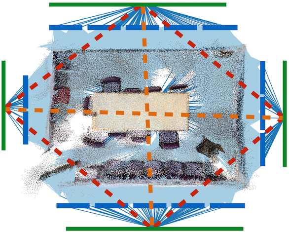
Creating Co-planarity Constraints. We first build a set of co-planarity constraints relating proxies in for each overlapping window of successive images. We do that by computing a global position for every planar proxy in using the current transformations . Then, for every window , we cluster co-planar proxies associated with features of images within the window using an agglomerative hierarchical clustering algorithm. Each coplanar set constitutes a new planar proxy that is inserted into , and co-planar, parent-child constraint is inserted into .
The constraints implied by are depicted for a single-room example in Figure 4. Note that shown is a late in the fine-to-coarse refinement, and thus the planar structures in the green span entire walls. In contrast to previous methods based on alignment to planes [25, 35, 49], it is possible to detect these large planar structures in our approach because previous iterations align overlapping subsets of the wall.
Creating Planar Relationship Constraints. We next build a set of structural constraints representing geometric relationships between parent planar proxies in the same or adjacent windows. Our goal is to detect salient relationships between planar structures (parallel, antiparallel, or orthogonal) that can help guide the optimization towards the correct registration.
We create a typed and weighted planar relationship for every pair of parent planar proxies ( and ) within the same window. Specifically, the type of the structural relationship and its weight are based on the angle between the normals. For parallel relationships the weight is defined as , for orthogonal , and for antiparallel . These weights are chosen so as to guide the registration when constraints are nearly met, but have little influence when they are not.
Creating Feature Correspondences. We next build a set of correspondence constraints between features detected in images within the same window. Following the general strategy of ICP, we construct correspondences between the closest compatible features for every pair of scans in every , where compatibility is determined by a maximum distance threshold, a maximum normal angle deviation, and a feature type check (planar features only match to planar features, etc.). No shape descriptors are used.
Since we expect images within the same window to become aligned as they are optimized, we set the maximum distance and maximum normal angle thresholds for rejecting outliers dynamically for every pair of images based on how many iterations they have been within the same window. The first time the two images are paired, the thresholds are quite large: 0.5m and 45 degrees. As the iterations proceed, they decrease linearly down to 0.15m and 20 degree.
Finally, for performance reasons, we subsample the set of correspondences created for all windows , such that the total number of them is equal to .
4.3 Optimization
The final processing step in each iteration is to optimize the camera transformations and planar proxies to minimize an error function encoding the detected constraints.
Our error function is a weighted sum of terms penalizing deformations of structural relationships (), warps of detected planes (), distances between corresponding features (), misalignments of local transformations (), and large changes in transformations ():
Planar Structure Error. is designed to encourage consistency between the registration and the the structural model:
where the three sub-terms account for coplanarity of hierarchical proxy relationships (), detected geometric relationships between proxies (), and fits of planar proxies to depth images (). The error due to coplanarity constraints is defined as:
where measures the deviation of two planar structures from coplanarity. The error in geometric relationships is:
where the and are normals of proxies , respectively. The error aligning planar proxies with depth images is:
where is the index of the image containing feature and is a number proportional to inliers of proxy , selected such that .
Feature Correspondence Error. is designed to encourage alignment of detected feature correspondences:
where , and , are the transformed positions and normals of features and .
Local Alignment Error. is designed to encourage pairwise transformations between adjacent frames to match the ones computed during preprocessing:
where and measures the misalignment of two transformations.
Inertia Error. is designed to encourage the transformations to remain approximately the same across iterations.
where represents the sum of squared differences between Euler angle rotations and translations for from one iteration to the next. This term has very low weight – it is added mainly to provide stability for the optimization and prevent the system of equations from being under-constrained.
5 Experimental Results
We performed a series of experiments designed to test the performance of the proposed method with comparisons to previous methods and ablation studies.
New Benchmark Dataset. RGB-D scans of indoor scenes with ground truth alignments are scarce. Most contain only part of a room [1, 9, 18, 23, 26, 36, 38], have less than ten test examples [9, 26, 47], or are based on synthetic data [18, 17]. As a result, the research community has compared registration results mainly on small, clean datasets that are not representative of the large real-world scans required for most applications.
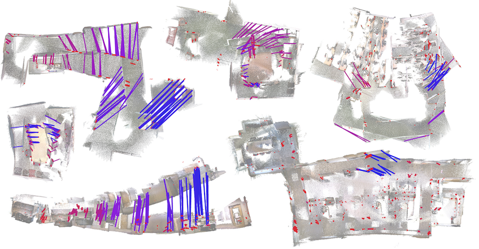
To address this issue, we introduce a new registration benchmark based on the SUN3D dataset [47]. SUN3D contains a large set RGB-D videos captured with a ASUS Xtion PRO LIVE sensor attached to a hand-held laptop in a variety of spaces (apartments, hotel rooms, classrooms, etc.). Each scan contains images, often covering multiple rooms. Previously, only eight of the scenes were released with full annotations and pose correction. Because of the lack of ground truth poses, these have not been used for quantitative evaluation of registration algorithms.
One of our contributions is to provide ground-truth point correspondences for 25 of the largest scenes in SUN3D. In all, we have manually clicked on 10,401 point correspondences with pixel-level accuracy. These ground-truth correspondences are largely in pairs of overlapping frames forming loop closures, but they also appear in pairs of nearby frames spread evenly through the scan, as shown in Figure 5. The average number of correspondences per scan is 416, with a minimum of 239 and a maximum of 714.
We use these ground truth correspondences to evaluate and compare RGB-D registration algorithms by computing their root mean squared error (RMSE). To quantify a lower bound on the RMSE in this test, we aligned the ground truth correspondences for all scene with no other constraints and report the errors in the left column of Table 1. Note that these lower-bounds are non-zero, even though clicked correspondences are pixel-accurate, due to the extreme noise in uncalibrated SUN3D depth maps.
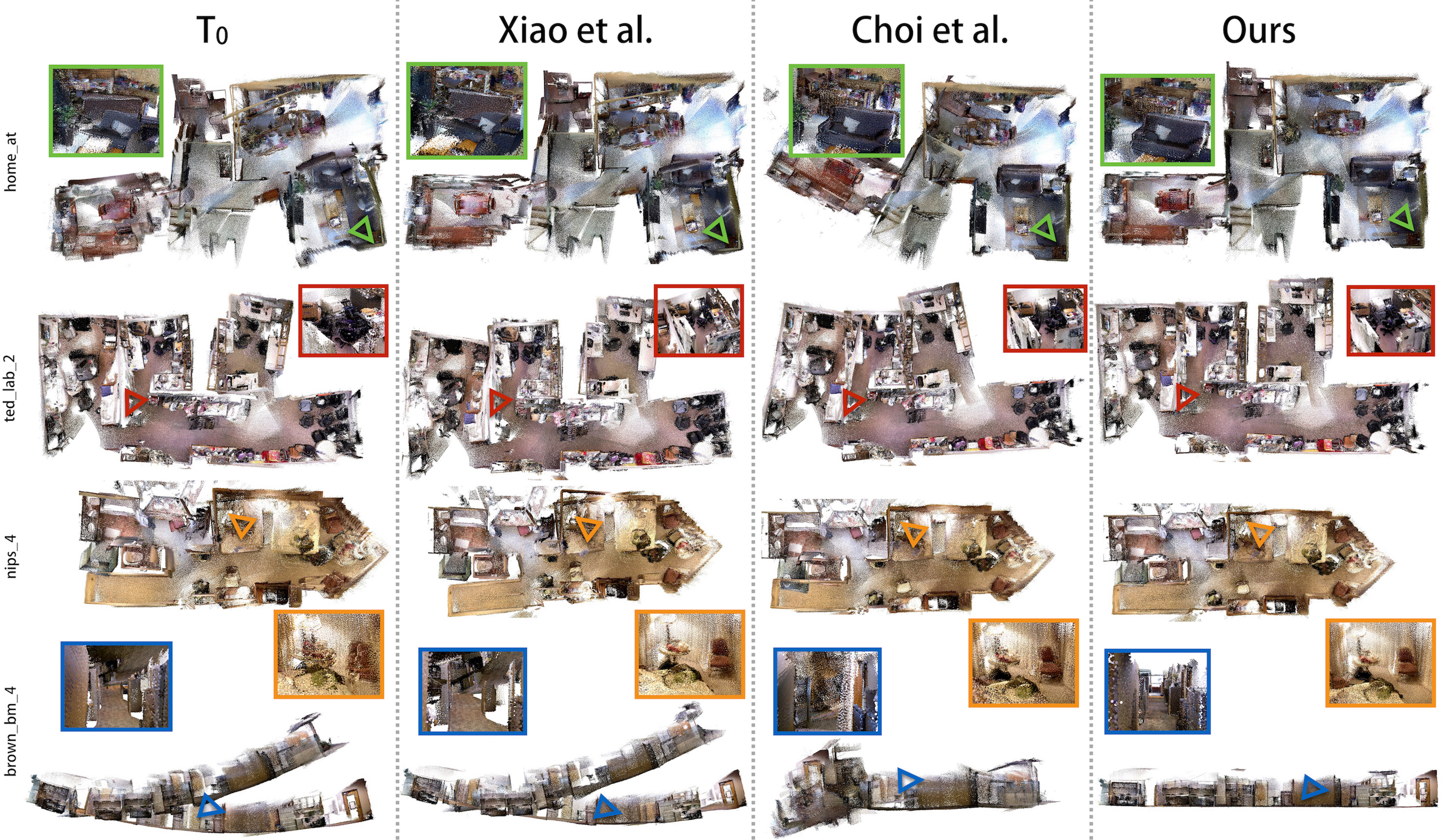
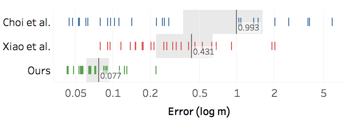
Comparisons to Previous Work. We evaluate our method in comparison to two prior methods for offline registration: Xiao et al.’s Sun3DSfm[48] and Choi et al.’s Robust Reconstruction of Indoor Scenes [8] (Figure 6). The first method by Xiao et al. uses the same method as we do for tracking camera poses, but also predicts loop closures via visual place recognition with a BoW approach and performs a global bundle adjustment to optimize for camera poses. The second method by Choi et al. fuses consecutive groups of 50 frames into fragments, aligns all pairs of fragments with a variant of RANSAC, selects pairs as potential loop closures, and then solves a least squares system of nonlinear equations that simultaneously solves for camera poses and loop closure weights. We believe this second method is the state-of-the-art for off-line global registration amongst ones with code available, even though it only uses the depth information. Comparisons are provided in the supplemental materials for several real-time reconstruction methods, which demonstrate worse performance than these off-line global methods.
| Ground Truth | Ours | Xiao et al. | Choi et al. | ||
| Average | 0.031 | 0.077 | 0.531 | 0.431 | 0.993 |
| Standard Deviation | 0.006 | 0.037 | 0.471 | 0.491 | 1.481 |
| Median | 0.031 | 0.065 | 0.421 | 0.255 | 0.224 |
| Minimum | 0.019 | 0.042 | 0.114 | 0.078 | 0.043 |
| Maxium | 0.045 | 0.221 | 2.124 | 2.007 | 5.819 |
Table 1 and Figure 7 show quantitative results for the comparison evaluated on our new SUN3D benchmark. Table 1 compares overall statistics of RMSEs for each algorithm, while Figure 7 shows the distributions of RMSEs. It can be seen in both of these results that our reconstruction algorithm aligns the ground truth correspondences better than either of the other two methods: our median error is 0.065m in comparison to 0.255m for Xiao et al. and 0.224m for Choi et al. In case-by-case comparisons, our method has the lowest error in 21 of 25 scenes.
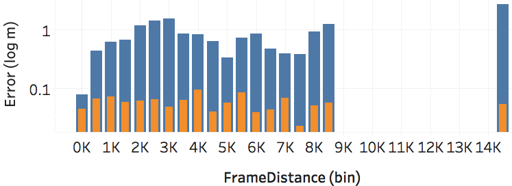
Investigating Fine-to-Coarse Iteration. To investigate the behavior of our fine-to-coarse algorithm, we computed histograms of distances versus frame index differences between pairs of frames linked by ground-truth correspondences. Figure 8 shows a comparison of these histograms for the registrations at the start of our algorithm (blue) and at the end (orange). It is interesting to note that our algorithm not only reduces the distances between ground-truth correspondences forming long-range loop closures (the right side of the plot), but also over short ranges. This demonstrates that the extracted structural model helps to fix not only global alignments, but also local ones.
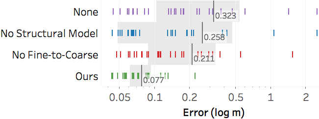
Ablation Studies. To investigate the value of our proposed a) fine-to-coarse iteration strategy and b) structural model, we performed comparisons of our method with all combinations of these methods enabled or disabled. The results in Figure 9 and 10 show that both provide critical improvements to the results. In particular, it is interesting to note that the fine-to-coarse iteration strategy improves ICP, even when no structural model is computed. This result highlights the value of aligning local structures before searching for loop closures at larger scales.
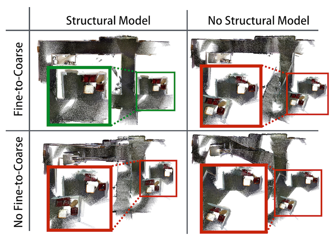
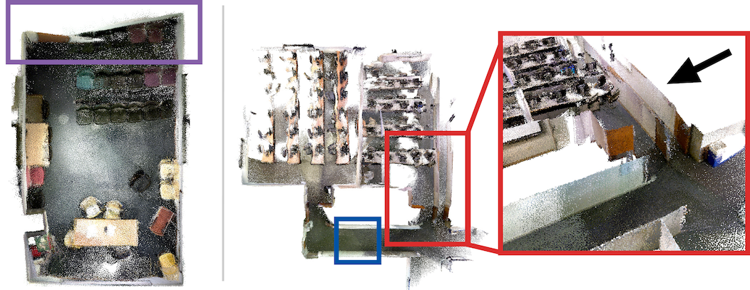
Failure Cases. Our method does not always succeed. For example, it can fail when multiple rooms are connected via featureless straight corridors and when rooms that are nearly (but not exactly) rectangular (Figure 11). Failures of the second type are rare – since the weight of enforcing parallelism and orthogonality constraints is low for pairs of planes at off-angles, we are able to reconstruct most scenes with non-Manhattan geometry correctly (as in the third row of Figure 7).
Timing. All our tests took less than an hour to finish on a machine with 3.0GHz processor and 128Gb of RAM. The shortest sequence of 875 frames took 108 seconds to complete, while the longest took 2,909 seconds for 14,915 frames.
6 Conclusions
This paper describes a method for global registration of RGB-D scans captured with a hand-held camera in a typical indoor environment. The key idea is a fine-to-coarse scheme that detects and enforces constraints (planar relationships and feature correspondences) within windows of gradually increasing scales in an iterative global optimization algorithm. The benefits of the proposed approach are demonstrated in experiments with a new benchmark for RGB-D registration, which contains 10,401 manually specified correspondences across 25 SUN3D scenes. This benchmark and all code will be publicly released to facilitate evaluation and comparison of future algorithms.
References
- [1] A. Anand, H. S. Koppula, T. Joachims, and A. Saxena. Contextually guided semantic labeling and search for 3d point clouds. IJRR, 2012.
- [2] A. Angeli, D. Filliat, S. Doncieux, and J.-A. Meyer. Fast and incremental method for loop-closure detection using bags of visual words. Robotics, IEEE Transactions on, 24(5):1027–1037, 2008.
- [3] A. Bartoli and P. Sturm. Constrained structure and motion from multiple uncalibrated views of a piecewise planar scene. International Journal of Computer Vision, 52(1):45–64, 2003.
- [4] P. J. Besl and N. D. McKay. A method for registration of 3-D shapes. IEEE Trans. PAMI, 14(2):239–256, 1992.
- [5] B. Brown and S. Rusinkiewicz. Global non-rigid alignment of 3D scans. ACM Transactions on Graphics (Proc. SIGGRAPH), 26(3), Aug. 2007.
- [6] J. Chen, D. Bautembach, and S. Izadi. Scalable real-time volumetric surface reconstruction. ACM Trans. Graph., 32(4):113:1–113:16, July 2013.
- [7] Z. Chen, O. Lam, A. Jacobson, and M. Milford. Convolutional neural network-based place recognition. arXiv preprint arXiv:1411.1509, 2014.
- [8] S. Choi, Q.-Y. Zhou, and V. Koltun. Robust reconstruction of indoor scenes. In IEEE Conference on Computer Vision and Pattern Recognition (CVPR), 2015.
- [9] A. Dai, M. Nießner, M. Zollhöfer, S. Izadi, and C. Theobalt. Bundlefusion: Real-time globally consistent 3d reconstruction using on-the-fly surface re-integration. arXiv preprint arXiv:1604.01093, 2016.
- [10] M. Dou, L. Guan, J.-M. Frahm, and H. Fuchs. Exploring high-level plane primitives for indoor 3d reconstruction with a hand-held rgb-d camera. In Asian Conference on Computer Vision, pages 94–108, 2012.
- [11] M. Dzitsiuk, J. Sturm, R. Maier, L. Ma, and D. Cremers. De-noising, stabilizing and completing 3d reconstructions on-the-go using plane priors. CoRR, abs/1609.08267, 2016.
- [12] H. E. Elghor, D. Roussel, F. Ababsa, and E. H. Bouyakhf. Planes detection for robust localization and mapping in rgb-d slam systems. In 3D Vision (3DV), 2015 International Conference on, pages 452–459, Oct 2015.
- [13] C. Estrada, J. Neira, and J. Tard´os. Hierarchical slam: Real-time accurate mapping of large environments. Transactions on Robotics, 21(4):588–596, 2005.
- [14] J. X. Fisher Yu and T. Funkhouser. Semantic alignment of lidar data at city scale. In 28th IEEE Conference on Computer Vision and Pattern Recognition, 2015.
- [15] U. Frese, P. Larsson, and T. Duckett. A multilevel relaxation algorithm for simultaneous localisation and mapping. IEEE Transactions on Robotics, 21(2):1–12, 2005.
- [16] G. Grisetti, R. Kümmerle, C. Stachniss, and W. Burgard. A tutorial on graph-based slam. IEEE Intelligent Transportation Systems Magazine, 2(4):31–43, 2010.
- [17] A. Handa, V. Patraucean, V. Badrinarayanan, S. Stent, and R. Cipolla. Scenenet: Understanding real world indoor scenes with synthetic data. In IEEE CVPR, 2016.
- [18] A. Handa, T. Whelan, J. McDonald, and A. Davison. A benchmark for RGB-D visual odometry, 3D reconstruction and SLAM. In IEEE Intl. Conf. on Robotics and Automation, ICRA, Hong Kong, China, May 2014.
- [19] P. Henry, M. Krainin, E. Herbst, X. Ren, and D. Fox. Rgb-d mapping: Using depth cameras for dense 3d modeling of indoor environments. In International Symposium on Experimental Robotics (ISER), 2010.
- [20] O. Kahler, V. A. Prisacariu, C. Y. Ren, X. Sun, P. H. S. Torr, and D. W. Murray. Very High Frame Rate Volumetric Integration of Depth Images on Mobile Device. IEEE Transactions on Visualization and Computer Graphics (Proceedings International Symposium on Mixed and Augmented Reality 2015, 22(11), 2015.
- [21] M. Keller, D. Lefloch, M. Lambers, S. Izadi, T. Weyrich, and A. Kolb. Real-time 3d reconstruction in dynamic scenes using point-based fusion. In 2013 International Conference on 3D Vision – 3DV, pages 1 – 8, DOI:10.1109/3DV.2013.9, June 2013.
- [22] M. Klingensmith, I. Dryanovski, S. Srinivasa, and J. Xiao. Chisel: Real time large scale 3d reconstruction onboard a mobile device. In Robotics Science and Systems 2015, July 2015.
- [23] K. Lai, L. Bo, and D. Fox. Unsupervised feature learning for 3d scene labeling. In IEEE International Conference on Robotics and Automation, page 3050–3057, 2014.
- [24] Y. Li, X. Wu, Y. Chrysanthou, A. Sharf, D. Cohen-Or, and N. J. Mitra. Globfit: Consistently fitting primitives by discovering global relations. ACM Transactions on Graphics, 30(4):52:1–52:12, 2011.
- [25] L. Ma, C. Kerl, J. Stueckler, and D. Cremers. Cpa-slam: Consistent plane-model alignment for direct rgb-d slam. In Int. Conf. on Robotics and Automation, 2016.
- [26] O. Mattausch, D. Panozzo, C. Mura, O. Sorkine-Hornung, and R. Pajarola. Object detection and classification from large-scale cluttered indoor scans. Computer Graphics Forum, 33(2):11–21, 2014.
- [27] A. Monszpart, N. Mellado, G. J. Brostow, and N. J. Mitra. Rapter: Rebuilding man-made scenes with regular arrangements of planes. ACM Trans. Graph., 34(4):103:1–103:12, July 2015.
- [28] R. A. Newcombe, A. J. Davison, S. Izadi, P. Kohli, O. Hillig̃es, J. Shotton, D. Molyneaux, S. Hodges, D. Kim, and . A. Fitzgibbon. Kinectfusion: Real-time dense surface mapping and tracking. In Mixed and augmented reality (ISMAR), 2011 10th IEEE international symposium on, pages 127–136. IEEE, 2011.
- [29] V. Nguyen, A. Harati, and R. Siegwart. A lightweight slam algorithm using orthogonal planes for indoor mobile robotics. In Intelligent Robots and Systems, 2007. IROS 2007. IEEE/RSJ International Conference on, pages 658–663. IEEE, 2007.
- [30] M. Nießner, M. Zollhöfer, S. Izadi, and M. Stamminger. Real-time 3d reconstruction at scale using voxel hashing. ACM Transactions on Graphics (TOG), 2013.
- [31] K. Pathak, A. Birk, N. Vaskevicius, and J. Poppinga. Fast registration based on noisy planes with unknown correspondences for 3-D mapping. IEEE Trans. Robotics, 26(3):424–441, June.
- [32] K. Pulli. Multiview registration for large data sets. In Proceedings of the 2Nd International Conference on 3-D Digital Imaging and Modeling, 3DIM’99, pages 160–168, Washington, DC, USA, 1999. IEEE Computer Society.
- [33] A. Ratter and C. Sammut. Local map based graph slam with hierarchical loop closure and optimisation. 2015.
- [34] S. Rusinkiewicz, O. Hall-Holt, and M. Levoy. Real-time 3D model acquisition. ACM Transactions on Graphics (Proc. SIGGRAPH), 21(3):438–446, July 2002.
- [35] R. Salas-Moreno, B. Glocken, P. Kelly, and A. Davison. Dense planar slam. In Mixed and Augmented Reality (ISMAR), 2014 IEEE International Symposium on, pages 157–164, Sept 2014.
- [36] N. Silberman, D. Hoiem, P. Kohli, and R. Fergus. Indoor segmentation and support inference from rgbd images. In Proc. European Conf. on Comp. Vision, 2012.
- [37] P. Stotko. State of the art in real-time registration of rgb-d images. In CESCG, 2016.
- [38] J. Sturm, N. Engelhard, F. Endres, W. Burgard, and D. Cremers. A benchmark for the evaluation of rgb-d slam systems. In Proc. of the International Conference on Intelligent Robot Systems (IROS), Oct. 2012.
- [39] Y. Taguchi, Y.-D. Jian, S. Ramalingam, and C. Feng. Point-plane slam for hand-held 3d sensors. In Robotics and Automation (ICRA), 2013 IEEE International Conference on, pages 5182–5189, May 2013.
- [40] Y. Tang and J. Feng. Hierarchical multiview rigid registration. Comput. Graph. Forum, 34(5):77–87, Aug. 2015.
- [41] A. Trevor, J. Rogers III, and H. Christensen. Planar surface SLAM with 3D and 2D sensors. In ICRA, 2012.
- [42] H. Wang, J. Wang, and L. Wang. Online reconstruction of indoor scenes from rgb-d streams. In IEEE CVPR, 2016.
- [43] J. Weingarten and R. Siegwart. 3D SLAM using planar segments. In IROS, page 3062–3067, 2006.
- [44] T. Whelan, M. Kaess, M. Fallon, H. Johannsson, J. Leonard, and J. McDonald. Kintinuous: Spatially extended KinectFusion. In RSS Workshop on RGB-D: Advanced Reasoning with Depth Cameras, Sydney, Australia, Jul 2012.
- [45] T. Whelan, M. Kaess, H. Johannsson, M. Fallon, J. Leonard, and J. McDonald. Real-time large scale dense RGB-D SLAM with volumetric fusion. Intl. J. of Robotics Research, IJRR, 2014.
- [46] T. Whelan, S. Leutenegger, R. F. Salas-Moreno, B. Glocker, and A. J. Davison. ElasticFusion: Dense SLAM without a pose graph. In Robotics: Science and Systems (RSS), Rome, Italy, July 2015.
- [47] J. Xiao, A. Owens, and A. Torralba. Sun3d: A database of big spaces reconstructed using sfm and object labels. Computer Vision, IEEE International Conference on, 0:1625–1632, 2013.
- [48] J. Xiao, A. Owens, and A. Torralba. SUN3D database: Semantic RGB-D bundle adjustment with human in the loop. In Proc. Int. Conf. on Comp. Vision, 2013.
- [49] Y. Zhang, W. Xu, Y. Tong, and K. Zhou. Online structure analysis for real-time indoor scene reconstruction. ACM Transactions on Graphics (TOG), 34(5):159, 2015.
- [50] Q.-Y. Zhou and V. Koltun. Dense scene reconstruction with points of interest. ACM Transactions on Graphics, 32(4), 2013.
- [51] Q.-Y. Zhou and V. Koltun. Color map optimization for 3d reconstruction with consumer depth cameras. SIGGRAPH Conf. Proc., 2014.
- [52] Q.-Y. Zhou and V. Koltun. Depth camera tracking with contour cues. In The IEEE Conference on Computer Vision and Pattern Recognition (CVPR), June 2015.