General background conditions for K-bounce and adiabaticity

Abstract

We study the background conditions for a bounce in a single scalar field model with a generalized kinetic term $K(X)$. At the background level we impose the existence of two turning points where the derivative of the Hubble parameter $H$ changes sign, a bounce point where the Hubble parameter vanishes. We find the conditions for $K(X)$ and the potential which ensure the above properties. We then give the examples of two models constructed according to these conditions. One is based on a quadratic $K$, and the other on a $K$ which is avoiding divergences of the second time derivative of the scalar field, which may otherwise occur. An appropriate choice of the initial conditions can lead to a sequence of consecutive bounces.

In ekpyrotic models, where the bounce occurs when the potential is not constant, large non adiabatic perturbations are produced, which can in turn source the growth of anisotropies. In the region where these models have a constant potential they became adiabatic on any scale, and because of this they may not conserve curvature perturbations on super-horizon scales.

I Introduction

The inflationary scenario provides a model able to explain many of the observational features of the observed Universe, such as the cosmic microwave background radiation isotropy or the the spatial flatness. An alternative scenario to solve the horizon problem is the possibility that the Universe underwent a contraction phase before the big-bang, i.e. a bounce. Several attempts have been made to understand if the bounce this could be a fully consistent cosmological model Gordon:2000hv ; Khoury:2009my ; Khoury:2001wf ; Lehners:2008vx ; Erickson:2003zm ; Khoury:2001bz ; Buchbinder:2007ad ; ArkaniHamed:2003uy ; Creminelli:2006xe ; Lehners:2007ac ; Creminelli:2007aq ; Xue:2011nw ; Cai:2012va ; Cai:2007qw , which could be a possible alternative to inflation.

In this paper we study the general condition to realize the bounce with a K-essence type scalar field, without introducing any additional field. We first obtain some general conditions on the the function $K(X)$ and the potential $V(\phi)$ and then give the examples of two models constructed according to these conditions. One is based on a quadratic $K(X)$, and the other on a $K(X)$ which is always avoiding divergences of the second time derivative of the scalar field, which may otherwise occur. An appropriate choice of the initial conditions can lead to a sequence of consecutive bounces.

In ekpyrotic models, where the bounce occurs when the potential is not constant, large non adiabatic perturbations are produced, which can in turn source the growth of anisotropies. In the region where these models have a constant potential they became adiabatic on any scale, and because of this they may not conserve curvature perturbations on super-horizon scales.

II $K(X)$-bounce

We will consider a scalar field with Lagrangian

$$L_{\phi}=\sqrt{-g}\left[K(X)-V(\phi)\right]\,\,\,,\,X=\frac{1}{2}g^{\mu\nu}\partial_{\mu}\phi\partial_{\nu}\phi$$ (1)

We denote the Planck mass with $m_{p}=(8\pi G)^{-1/2}$, and we adopt adopt units in which $8\pi G/3=1$, so that the Einstein’s equation take the form

$$H^{2}=\rho \dot{H}=-\frac{3}{2}(\rho+P)=\frac{3}{2}(K+T)=-3K^{\prime}X$$ , (2)

where the energy density and pressure are

$$\rho = 2K^{\prime}X-K+V=T+V\,,$$ (3)

$$P = K-V\,.$$ (4)

In the above equations we have introduced the function $T(x)$

$$T(X) = 2K^{\prime}X-K\,,$$ (5)

because it is convenient to express the equations of motion in terms of it, and it plays a crucial role in the existence of smooth solutions as we will show later.

The energy conservation equations can then give the equation of motion of the scalar field

$$T^{\prime}\ddot{\phi}+3HK^{\prime}\dot{\phi}+V^{\prime} = 0\,.$$ (6)

The minimally coupled scalar field equation of motion corresponds to the case when $K(X)=T(X)=X$.

Another important quantity to determine the dynamics of the universe is the second derivative of $H$

$$\ddot{H} = -(3K^{\prime}\dot{\phi}\ddot{\phi}+\frac{3}{2}\dot{\phi}^{3}K^{\prime\prime}\ddot{\phi})\,,$$ (7)

which after substituting the equation of motion for $\ddot{\phi}$ gives

$$\ddot{H} = \frac{3\left(\dot{\phi}^{3}K^{\prime\prime}+2\dot{\phi}K^{\prime}\right)\left(3H\dot{\phi}K^{\prime}+V^{\prime}\right)}{2\left(\dot{\phi}^{2}K^{\prime\prime}+K^{\prime}\right)}$$ (8)

We now define turning points the local extrema of $H(t)$, where $\dot{H}=0$. From the Einstein equations we know that $\dot{H}$ can be zero either because $K^{\prime}=0$ or $X=0$, and the corresponding value of the second order time derivative $\ddot{H}$ will play a crucial role in determining if these are actual extrema or flex points. From the previous equation after substituting respectively $K^{\prime}=0$ or $X=0$ we get

$$X=0\, : \ \ddot{H}=0\,$$ (9)

$$K^{\prime}=0\, : \ \ddot{H}=\frac{3}{2}V^{\prime}\dot{\phi}\,$$ (10)

This implies that $X=0$ is a flex point and consequently can never be a turning point, while points at which $K^{\prime}=0$ can be either local maxima or minima depending on the relative sign of $V^{\prime}$ and $\dot{\phi}$.

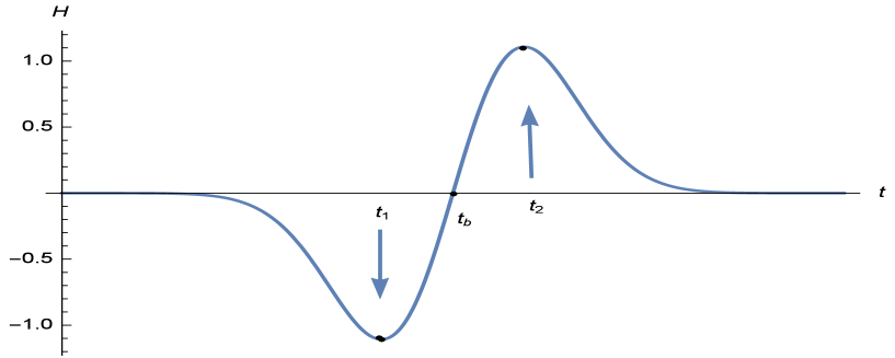
For a bounce with dynamics similar to the one shown in fig.(1) to occur, the following three critical points are necessary:

$$t_{1}\,:\dot{H}=0,\ddot{H}>0 \rightarrow K^{\prime}_{1}=0\,,V^{\prime}_{1}\dot{\phi}_{1}>0\,,$$ (11)

$$t_{b}\,:\dot{H}>0,H=0, \rightarrow K^{\prime}_{b}<0\,,\rho=0\,,$$ (12)

$$t_{2}\,:\dot{H}=0,\ddot{H}<0 \rightarrow K^{\prime}_{2}=0\,,V^{\prime}_{2}\dot{\phi}_{2}<0\,.$$ (13)

where we have defined

$$K^{\prime}_{i}=K^{\prime}(X(t_{i}))\,,V^{\prime}_{i}=V^{\prime}(\phi(t_{i}))\,,\dot{\phi}_{i}=\dot{\phi}(t_{i})$$ (14)

and $\{t_{1},t_{2}\}$ correspond to the first and second turning point times, while $t_{b}$ is the bounce time. The existence of a solution able to satisfy the above requirements will be studied in the following sections.

Figure 1: Schematic representation of the evolution of $H(t)$ around the bounce. There are two turning points at which the derivative $\dot{H}(t_{1})=\dot{H}(t_{2})$ is zero, and a bounce point where $H(t_{b})=0$

II.1 An example: quadratic bounce

Based on the background conditions derived in the previous section we can introduce a quadratic kinetic term model and an appropriate potential which will give the correct dynamic for $H(t)$:

$$K(X) = (X-X_{T})^{2}$$ (15)

$$V(\phi) = \frac{1}{2}\left[e^{x^{2}}-0.2e^{-\left(\frac{x}{2}\right)^{2}}\right]$$ (16)

It is convenient to define ${\mathcal{H}}^{2}_{0}$ as the phase space locus of the points where the energy density is zero, i.e. the set of points satisfying the equation

$$3H^{2}=\rho(X,\phi)= T(X)+V(\phi)=0$$ (17)

.

Figure 2: The potential for the model in eq.(16) is plotted as a function of the $\phi$ in units of $m_{p}^{2}$.

Figure 3: The zero energy locus ${\mathcal{H}}^{2}_{0}$ locus is plotted for the model defined in eq.(16). The region below this curve is physically impossible, since it corresponds to $H^{2}<0$. Physical phase space trajectories can only be above this line, or be tangent to it at the time of the bounce, has proofed in the appendix.

Figure 4: The phase space trajectory of the solution of the differential equations for the model defined in eq.(16) is plotted in blue. The red line corresponds to the ${\mathcal{H}}^{2}_{0}$ locus where the energy is zero. As it can be seen the phase space trajectory is tangent to ${\mathcal{H}}^{2}_{0}$ at the bounce time, as proofed in the appendix. The scalar field is plotted in units of $m_{p}^{2}$ and $X$ in in units of $m_{p}^{4}$.

Figure 5: H is plotted as function of time in units of $m_{p}^{-1}$ for the model defined in eq.(16)

Figure 6: The scalr field $\phi$ is plotted as a function of time in units of $m_{p}^{-1}$ for the model defined in eq.(16).

Figure 7: $X(t)$ is plotted as a function of time in units of $m_{p}^{2}$ for the model defined in eq.(16).

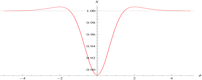
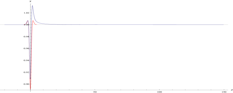
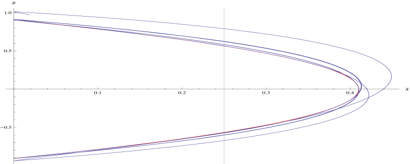
The phase space behavior of the model defined in eq.(16) is shown in fig.(2,3,4,6,7). As can be seen in fig.(3,4) the phase space trajectory is tangent to the zero energy locus ${\mathcal{H}}2_{0}$ at the bounce time, as proofed in the appendix. The turning points correspond to $X=X_{T}=X(t_{1})=X(t_{2})$, and the sign of $V^{\prime}_{i}\dot{\phi}_{i}$ determine, according to eq.(11,13), if the turning point is a local minimum or maximum for $H(t)$.

III Possible divergences of the second derivative of $\phi$

In this section we will try to construct some other model satisfying the conditions in eq.(14). Let’s consider models of the type

$$K(X) = (X-X_{T})^{2}$$ (18)

$$V(\phi) = \frac{1}{2}m^{2}\phi^{2}$$ (19)

where $X_{T}$ the value of $X$ at which the turning point for H should occur, i.e. where $K^{\prime}(X_{T})=0$, based on the considerations in the previous section. Note that in this case we have $X_{T}=X(t_{1})=X(t_{2})$, but $V_{1}\dot{\phi_{1}}\neq V_{2}\dot{\phi_{2}}$ in order to satisfy the conditions for the turning points given in eq.(11,13). The problem with this kind of model is that there is a line in phase space plan where $T^{\prime}(X_{c})=0$, which corresponds to a divergence of the second derivative of $\phi$. At that point the equation of motion becomes a first order equation, which correspond to a constraint of the value of the field $\phi_{c}$ when $X=X_{c}$. This critical point in phase space is defined by the following conditions:

$$T^{\prime}(X_{c}) = 0\,,$$ (20)

$$\frac{3[K(X_{c})+T(X_{c})]\sqrt{T(X_{c})+V(\phi_{c})}}{\sqrt{2X_{c}}}+V_{c}^{\prime} = 0\,.$$ (21)

These equations can be solved to give

$$X_{c} = \frac{X_{T}}{3}\,,$$ (22)

$$\phi_{c} = -\frac{8\sqrt{\frac{2}{3}}{X_{T}}^{5/2}}{\sqrt{-3+16{X_{T}}^{3}}}\,.$$ (23)

To avoid this kind of divergence we will introduce a new class of models in the next section.

IV Models avoiding the divergence of the second derivative

In order to avoid the degenerate solutions encountered in the model studied in the previous section we consider a class of models for which $T^{\prime}(X)$ is never zero

$$T^{\prime}(X)=a$$ (24)

where $a$ is a constant. Solving for $K(X)$ the above differential equation we get

$$K(X) = aX+b\sqrt{X}+c$$ (25)

where $b$ and $c$ are two arbitrary integration constants. The so cuscuton model Afshordi:2006ad corresponds to the case in which $a=0$. In this case both $T$ and $T^{\prime}$ vanish.

The terms proportional to $\sqrt{X}$ plays a crucial role in allowing the bounce dynamics because without it the it would be difficult to define a not divergent $K$ with a minim for positive $X$. This will be shown in details later. In order to obtain a $K(X)$ with a local minimum we need a negative $b<0$, leading to a minimum at

$$X_{T} = \frac{b^{2}}{4}$$ (27)

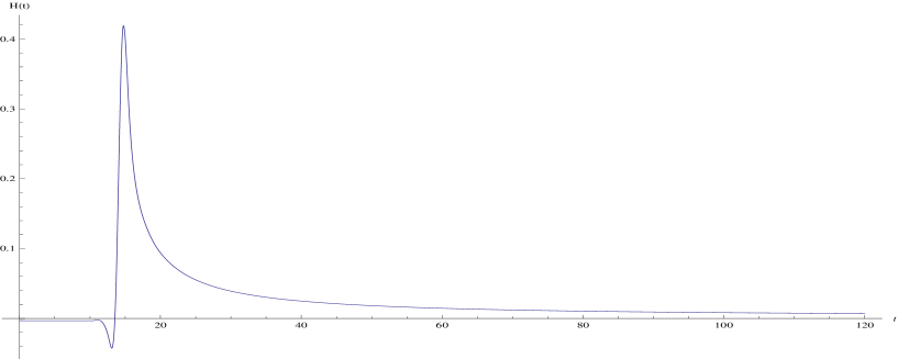
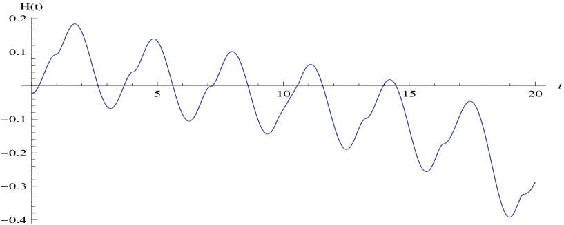
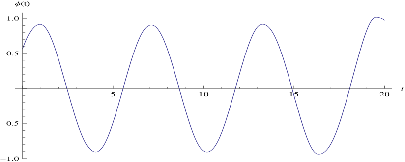
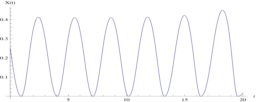
The following figures show the solutions of the differential equations for $H(t)$ and $\phi(t)$ for a the specific case. Not that an oscillatory $H(t)$ can be obtained for an appropriate choice of the initial conditions, leading to a sequence of consecutive bounces.

Also note that the linear part of $K(X)$ can give a an ekpyrotic phase, and it arises naturally by imposing the condition $T^{\prime}(X)=a$ The phase space behavior of the model defined in eq.(16) is shown in fig.(9,8,10,11). As can be seen in fig.(LABEL:H2V2,8) the phase space trajectory is tangent to the zero energy locus ${\mathcal{H}}2_{0}$ at the bounce time, as proofed in the appendix. As in the case of the model defined in eq.(16) the turning points correspond to $X=X_{T}=X(t_{1})=X(t_{2})$, and the sign of $V^{\prime}_{i}\dot{\phi}_{i}$ determine, according to eq.(11,13), if the turning point is a local minimum or maximum for $H(t)$.

$$K(X) = X-\sqrt{X}$$ (28)

$$K^{\prime}(X_{T})=0 \,; X_{T}=\frac{1}{4}$$ (29)

$$V_{2}(\phi) = V_{0}+\frac{1}{2}\phi^{2}$$ (30)

Figure 8: Space phase trajectory of the solution of the differential equations for the scalar field $\phi$ is plotted in blue for the model in eq.(29), with $V_{0}=-0.41m_{p}^{4}$. The red line corresponds to the zero energy locus ${\mathcal{H}}^{2}_{0}$. The vertical line is for $X=X_{t}$, the minimum of $K$ where $K^{\prime}(X_{T})=0$, which corresponds to a turning point for $H(t)$. The points at which the field trajectory is touching the zero energy locus correspond to the bounce times. The scalar field is plotted in units of $m_{p}^{2}$ and $X$ in in units of $m_{p}^{4}$.

Figure 9: H is plotted as function of time in units of $m_{p}^{-1}$ for the model defined in eq.(cusB)

Figure 10: The scalar field $\phi$ is plotted as function of time in units of $m_{p}^{-1}$ for the model defined in eq.(29).

Figure 11: $X(t)$ is plotted as a function of time in units of $m_{p}^{4}$ for the model defined in eq.(29).

V Stability of cosmological perturbations and adiabaticity

So far we have focused on the conditions to realize the bounce at the background level, but in order for these models to be viable cosmological models which could provide an alternative to inflation, we need to check if the cosmological perturbations are stable. In particular there could be problems with the growth of anisotropies Xue:2011nw , or gradient instabilities could arise. These kind of instabilities could be healed by introducing additional terms parts, such as Galileion terms, to the Lagrangian. We will leave a detailed study of the stability of cosmological perturbation to a future upcoming work, since the purpose of the present paper is mainly the derivation of general conditions to realize the bounce at the background level with a $K(X)$ model.

Due to the form of the Lagrangian we can nevertheless anticipate that the behavior of curvature perturbations for these models requires a careful treatment. The non-adiabatic pressure perturbation for these kind of scalar field models is in fact zero on any scales Romano:2016gop in the region where the potential is constant, because in that regime they are equivalent to a barotropic fluid with equation of state $P(\rho)$ so that

$$\delta P_{nad}=\delta P-\frac{\dot{P}}{\dot{\rho}}=0$$ (32)

For this reason they are called globally adiabatic(GA) models, to distinguish them from attractor models which are adiabatic only on super-horizon scales (SHA).

After defining the perturbed metric as

$$ds^{2} = a^{2}\Bigl{[}-(1+2A)d\eta^{2}+2\partial_{j}Bdx^{j}d\eta$$ (33)

$$\qquad+\left\{\delta_{ij}(1+2{\mathcal{R}})+2\partial_{i}\partial_{j}E\}dx^{i}dx^{j}\right\}\Bigr{]}\,.$$

in Romano:2015vxz it was shown that in general relativity, in absence of anisotropies, the conservation of the perturbed energy momentum tensor gives

$$\delta P_{nad}=\left[\left(\frac{c_{w}}{c_{s}}\right)^{2}-1\right](\rho+P)\frac{\dot{{\mathcal{R}}_{c}}}{H}.$$ (34)

which is true on any scale, and is not based on neglecting any gradient term. For GA models the adiabatic sound speed $c_{s}=\frac{\partial P}{\partial\rho}$ is equal to the phase speed $c_{w}=\frac{\dot{P}}{\dot{\rho}}$ and for this reason, despite $\delta P_{nad}=0$, nothing can be inferred about the behavior of $\dot{{\mathcal{R}}_{c}}$, otherwise ${\mathcal{R}}_{c}$ should be constant on any scale. Based on eq.(34) we can deduce that since in ekpyrotic models the potential is not constant during the bouncing phase, $c_{s}\neq c_{w}$. The exponential growth of ${\mathcal{R}}_{c}$ Xue:2011nw then implies that $\delta P_{nad}\neq 0$, i.e. the bounce is strongly non adiabatic. This large non adiabaticity is in fact the cause of the growth of anisotropies during the bouncing phase.

On the contrary, in the region where the potential asymptotes a constant value, these models could enter a phase of ultra-slow inflation in which curvature perturbations may not be conserved on super-horizon scales Romano:2016gop . A similar ultra-slow phase could occur for the model defined in eq.(16), in the region where the potential tends to a constant value.

VI Conclusion

We have derived the general conditions to obtain a bounce with a scalar field model with generalized kinetic term of the form $K(X)$ in general relativity. The requirement of the existence of a bounce point and of two turning points for $H(t)$ give some conditions which $K(X)$ and the potential $V(\phi)$ have to satisfy. We have given the examples of two models constructed according to these conditions. One is based on a quadratic $K(X)$, and the other on a $K(X)$ which is always avoiding divergences of the second time derivative of the scalar field, which may otherwise occur. An appropriate choice of the initial conditions can lead to a sequence of consecutive bounces.

In ekpyrotic models, where the bounce occurs when the potential is not constant, large non adiabatic perturbations are produced, which can in turn source the growth of anisotropies. In the region where these models have a constant potential they became adiabatic on any scale, and because of this they may not conserve curvature perturbations on super-horizon scales.

In the future it will be interesting to study in details the cosmological perturbations during and after the bounce, and in particular the effects of global adiabaticity in the region where the potential tends to a constant value.

Appendix A Phase space trajectory and zero energy locus

In general the slope of the tangent at a given point along the trajectory in phase space is

$$m = \frac{d\phi}{dX}=\frac{\dot{\phi}}{\dot{X}}=\frac{1}{\ddot{\phi}}$$ (35)

From the equation of motion for $\phi$ we get that at the bounce, when $H=0$

$$\ddot{\phi_{b}}=-\frac{V^{\prime}(\phi_{b})}{T^{\prime}(X_{b})}$$ (36)

implying that the phase space trajectory at the time of the bounce has slope

$$m_{b} = -\frac{T^{\prime}(X_{b})}{V^{\prime}(\phi_{b})}\,.$$ (37)

It is convenient to define ${\mathcal{H}}^{2}_{0}$ as the phase space locus of the points where the energy density is zero, i.e. the set of points satisfying the equation

$$3H^{2}=\rho(X,\phi)= T(X)+V(\phi)=0$$ (38)

and then we can get the equation defining ${\mathcal{H}}_{0}$ in the form $\phi(X)$ as

$$\phi_{{\mathcal{H}}_{0}}(X) = V^{-1}(-T(X))\,.$$ (39)

The slope of the tangent to ${\mathcal{H}}_{0}$ is then given as function of $X$ by

$$m_{{\mathcal{H}}_{0}}(X) = \frac{d\phi_{{\mathcal{H}}_{0}}}{dX}=\frac{dV^{-1}(-T)}{dT}\frac{dT}{dX}=-\frac{T^{\prime}(X)}{V^{\prime}(V^{-1}(-T))}=-\frac{T^{\prime}(X)}{V^{\prime}(\phi_{{\mathcal{H}}_{0}}(X))}\,,$$ (40)

where we have used eq.(39) and expressed the derivative of the inverse function $V^{-1}$ in terms if $V^{\prime}$.

From this we immediately deduce that any scalar field phase space trajectory reaching ${\mathcal{H}}_{0}$ at a point $(X_{b},\phi_{b}=\phi_{{\mathcal{H}}_{0}}(X_{b}))$ is tangent to ${\mathcal{H}}_{0}$ at that point since

$$m_{b}=-\frac{T^{\prime}(X_{b})}{V^{\prime}(\phi_{b})}=-\frac{T^{\prime}(X_{b})}{V^{\prime}(\phi_{{\mathcal{H}}_{0}}(X_{b}))}=m_{{\mathcal{H}}_{0}}(X_{b})\,.$$ (41)

This result is valid for any $K(X)$, and it ensures that only positive energy trajectories are dynamically allowed, since when the scalar field reaches ${\mathcal{H}}_{0}$ it is always tangent to it, and never crosses it, which would imply entering the unphysical phase space region where $H^{2}<$