Phenomenology of 2HDM with VLQs

Abstract

In this paper, we examine the consistency of the Large Hadron Collider (LHC) data collected during Run 1 and 2 by the ATLAS and CMS experiments with the predictions of a 2-Higgs Doublet Model (2HDM) embedding Vector-Like Quarks (VLQs) for $pp\to H,A$ production and $H,A\to\gamma\gamma$ decay mechanisms, respectively, of (nearly) degenerate CP-even ($H$) and CP-odd ($A$) Higgs bosons. We show that a scenario containing one single VLQ with Electro-Magnetic (EM) charge $2/3$ can explain the above ATLAS and CMS data for masses in the region 350 GeV $\leq m_{\rm VLQ}\leq 1.5$ TeV or so, depending on $\tan\beta$, and for several values of the mixing angle between the top quark ($t$) and its VLQ counterpart ($T$). We then perform a global fit onto the model by including all relevant experimental as well as theoretical constraints. The surviving samples of our analysis are discussed within 2$\sigma$ of the LHC measurements. Additionally, we also comment on the recent anomalous result reported by CMS using Run 2 data on the associated Standard Model (SM) Higgs boson production with top quark pairs $pp\to t\bar{t}h$ with an observed significance of 3.3$\sigma$. Other than these specific examples, we also present a phenomenological analysis of the main features of the model, including the most promising $T$ decay channels.

I Introduction

After the Higgs boson discovery in Run 1 of the Large Hadron Collider (LHC) at CERN Aad:2012tfa ; Chatrchyan:2012xdj , the ATLAS and CMS collaborations have carried out a broad programme looking for new physics Beyond the Standard Model (BSM) at the TeV scale. In particular, they have developed a powerful detection machinery of spin-0 resonances. However, new physics phenomena might take different forms from those established so far and, once discovered, they will require a complementary effort in order to understand their underlying nature. In fact, there are already several potential anomalies in the Run 1 Higgs data indicating possible deviations from the SM expectations in the Higgs sector. In particular, the signal strength of the $t\bar{t}h$ associated production mode is the most prominent one, while milder effects are seen in the fits to those extracted from the other production modes active at the LHC, i.e., gluon-gluon scattering (ggh), Higgs-strahlung (hV) and Vector Boson Fusion (VBF).

A possibility to capture at once all such anomalies is offered by the presence of Vector-Like Quark (VLQs) as they can, on the one hand, affect the SM-like Higgs (henceforth denoted by $h$) production and decay phenomenology (as they would enter the loops mediating the processes $gg\to h$ as well as $h\to\gamma\gamma$ and $Z\gamma$) and, on the other hand, mediate a $t\bar{t}h$ final state (tth). Intriguingly, the same VLQs affecting $h$ processes would also do so for heavier Higgs states, which may pertain to a BSM scenario. To be specific in defining our framework, we investigate the effects of VLQs in the production and decay of Higgs bosons within a 2-Higgs Doublet Model type-II (2HDM-II). In practice, we concentrate here on new states of matter that are heavy spin 1/2 particles that transform as triplets under color but, unlike SM quarks, their left- and right-handed couplings have the same Electro-Weak (EW) quantum numbers. Furthermore, their couplings to Higgs bosons do not participate in the standard EW Symmetry Breaking (EWSB) dynamics onset by the Higgs mechanism, hence they are not of Yukawa type (i.e., proportional to the mass), rather they are additional parameters, which can then be set as needed in order to achieve both compliance with present data and predict testable signals for the future.

The ATLAS and CMS collaborations, while collecting data at 7, 8 and 13 TeV, performed searches for VLQs with different quantum numbers, probing single and pair production mechanisms, as well as decay modes into all three generations of SM quarks (for the most updated experimental results of ATLAS and CMS we refer to the respective web pages twikiATLAS8TeV ; twikiATLAS13TeV ; twikiCMS ). However, new extra quarks can be charged under new symmetries, like $T$-parity in Little Higgs ArkaniHamed:2002qx ; Cheng:2003ju ; Cheng:2004yc ; Low:2004xc ; Hubisz:2004ft ; Cheng:2005as ; Hubisz:2005tx and Kaluza-Klein parity in Extra Dimension Antoniadis:1990ew ; Appelquist:2000nn ; Servant:2002aq ; Csaki:2003sh ; Cacciapaglia:2009pa models. Such VLQs have been searched for at both the Tevatron Aaltonen:2011rr ; Aaltonen:2011na and LHC ATLAS:2011mda ; CMS:2012dwa , though no evidence for the existence of other quarks, beside those of the SM, has been obtained. Direct bounds on heavy chiral quarks can be interpreted as bound on VLQs, but it must be stressed that decay channels of VLQs are different from decay channels of heavy chiral quarks Barducci:2017xtw . Thus, if the VLQs have a strong mass degeneracy, the visible decay products of the VLQ are too soft to be detected and, as a consequence, the bounds on the VLQ mass can be very weak, analogous to the case of strong degeneracy between squarks and neutralinos in supersymmetry. Intriguingly, as we shall detail below, even in our simple scenario, VLQ mass values down to 400 GeV are still possible, so that they could strongly affect, e.g., the $gg\to h\to V\gamma$ (with $V=\gamma,Z$) rates.

Now, let us also assume that additional (pseudo)scalar objects possibly behind the LHC experimental data do originate from the same EWSB mechanism governing the generation of the $\approx 125$ GeV Higgs state. This is indeed a possibility not excluded by current theoretical and experimental constraints. Under these circumstances, it is then of phenomenological importance to consider the case of a second Higgs doublet participating in EWSB alongside the one responsible for the discovered Higgs state. This mass generation dynamics is well known in the form of 2HDMs Branco:2011iw . We are therefore left with a new physics construct that would include a 2HDM supplemented by one or more VLQs as a potential scenario that could accommodate the LHC data on the $\approx 125$ GeV Higgs boson and additionally explain results above the SM yield.

In this paper, we wish to build on the results of Benbrik:2015fyz ; Aguilar-Saavedra:2013qpa ; Badziak:2015zez ; Angelescu:2015uiz , where a similar possibility was discussed (by some of us), in which the role of a 2HDM was played by a SM-like Higgs doublet supplemented by an additional Higgs singlet. We intend to review here a 2HDM plus single VLQ scenario, where the VLQ has the same Electro-Magnetic (EM) charge of the top quark (with which it then mixes), as a candidate to study the implications of the heavy Higgs searches by the ATLAS and CMS collaborations both with 8 TeV and the latest 13 TeV data. Furthermore, we will relate such data samples to those involving $\gamma\gamma$ and $Z\gamma$ final states. In addition, we will show an enhancement of the $pp\to t\bar{t}h$ cross-section at the LHC induced by small mixing of the top quark with the additional state $T$. Finally, we will discuss the possibility of VLQs produced as real objects in the detector decaying into Higgs boson states, both neutral and charged.

Our paper is formatted as follows. In the next section, we describe in some detail the model concerned. In the three subsequent sections, we present our results, followed by our conclusions.

II A 2HDM extended by an up-type vector-like quark

A simple extension of the SM is the well-known 2HDM that expands the Higgs sector of the SM by an additional Higgs doublet. The spectrum of the model contains additional Higgses and possesses an alignment limit Carena:2013ooa , in which one of the Higgses completely mimics the SM one.
To describe our model, we start with the well known CP-conserving 2HDM scalar potential for ($\Phi_{1},\Phi_{2})$ with a discrete symmetry $\Phi_{1}\to-\Phi_{1}$ that is only violated softly by dimension two terms Branco:2011iw ; Gunion:1989we :

$$V\left(\Phi_{1},\Phi_{2}\right) = m_{11}^{2}\Phi_{1}^{\dagger}\Phi_{1}+m_{22}^{2}\Phi_{2}^{\dagger}\Phi_{2}-m_{12}^{2}\left(\Phi_{1}^{\dagger}\Phi_{2}+\Phi_{2}^{\dagger}\Phi_{1}\right)$$ (1)

$$+ \frac{\lambda_{1}}{2}\left(\Phi_{1}^{\dagger}\Phi_{1}\right)^{2}+\frac{\lambda_{2}}{2}\left(\Phi_{2}^{\dagger}\Phi_{2}\right)^{2}+\lambda_{3}\left(\Phi_{1}^{\dagger}\Phi_{1}\right)\left(\Phi_{2}^{\dagger}\Phi_{2}\right)$$

$$+ \lambda_{4}\left(\Phi_{1}^{\dagger}\Phi_{2}\right)\left(\Phi_{2}^{\dagger}\Phi_{1}\right)+\frac{\lambda_{5}}{2}\left[\left(\Phi_{1}^{\dagger}\Phi_{2}\right)^{2}+\left(\Phi_{2}^{\dagger}\Phi_{1}\right)^{2}\right],$$

where all parameters are real. The two complex scalar doublets $\Phi_{1,2}$ may be rotated into a basis, $H_{1,2}$, where only one obtains a Vacuum Expectation Value (VEV),

$$H_{1}=\left(\begin{array}[]{c}G^{+}\\ \frac{v+\varphi^{0}_{1}+iG^{0}}{\sqrt{2}}\\ \end{array}\right),\quad H_{2}=\left(\begin{array}[]{c}H^{+}\\ \frac{\varphi^{0}_{2}+iA}{\sqrt{2}}\\ \end{array}\right),$$ (6)

where $G^{0}$ and $G^{\pm}$ are the would-be Goldstone bosons and $H^{\pm}$ are a pair of charged Higgses. Herein, $A$ is a CP-odd pseudoscalar which does not mix with the other neutral states in the CP-conserving case. The physical CP-even scalars $h$ and $H$ are mixtures of $\varphi^{0}_{1,2}$ and the scalar mixing is parameterized as

$$\left(\begin{array}[]{c}h\\ H\\ \end{array}\right)=\left(\begin{array}[]{cc}s_{\beta-\alpha}&c_{\beta-\alpha}\\ c_{\beta-\alpha}&-s_{\beta-\alpha}\\ \end{array}\right)\left(\begin{array}[]{c}\varphi^{0}_{1}\\ \varphi^{0}_{2}\\ \end{array}\right),$$ (13)

where $\tan\beta=v_{2}/v_{1}$ is the angle used to rotate $\Phi_{1,2}$ into $H_{1,2}$ and $\alpha$ is the additional mixing needed to diagonalize the CP-even mass matrix. As mentioned in the introduction, in order to alter the gluon-gluon-Higgs, photon-photon-Higgs and/or $Z$-photon-Higgs couplings, one can advocate the inclusion of new heavy fermions such as a VLQ partner of the top quark with the same EM charge. In fact, there are many SM extensions that require vector-like fermions in their spectrum (for an overview see Ellis:2014dza ; Aguilar-Saavedra:2013qpa ). Such a new VLQ will mix with the top quark through the Yukawa interactions and can contribute, therefore, to some SM observables. To derive these new interactions, we first study the Yukawa sector within a 2HDM extended by a VLQ pair $(T_{L},T_{R})$ in the $\mathbf{1}_{2/3}$ representation of the SM EW group. In the 2HDM-II, our concern here, one doublet couples to up quarks and the other one couples to down quarks and charged leptons. The most general renormalizable model for the quark Yukawa interactions and mass terms can be described, limited to third generation quarks and new VLQs, by the following Lagrangian,

$$-\mathcal{L}_{Y}^{II} \supset y_{T}\overline{Q_{L}^{0}}\widetilde{H}_{2}T_{R}^{0}+\xi_{T}\overline{Q^{0}_{L}}\widetilde{H}_{1}T_{R}^{0}+M_{T}\overline{T_{L}^{0}}T_{R}^{0}$$ (18)

$$\supset y_{T}(\overline{t_{L}^{0}},\overline{b_{L}^{0}})\left(\begin{array}[]{c}\frac{\varphi^{0}_{2}-iA}{\sqrt{2}}\\ -H^{-}\\ \end{array}\right)T_{R}^{0}+\xi_{T}(\overline{t_{L}^{0}},\overline{b_{L}^{0}})\left(\begin{array}[]{c}\frac{v+\varphi^{0}_{1}-iG^{0}}{\sqrt{2}}\\ -G^{-}\\ \end{array}\right)T_{R}^{0}+M_{T}\overline{T_{L}^{0}}T_{R}^{0}+\rm{h.c},$$

where $\tilde{H}_{i}\equiv i\tau_{2}H^{*}_{i}$ ($i=1,2$), $Q^{0}_{L}$ are the SM quark doublets and the $u^{i}_{R}$’s are the SM up-type quark singlets. Note that additional kinetic mixing terms of the form $\overline{T_{L}}t^{i}_{R}$ can always be rotated away and reabsorbed into the definition of $y_{t,T}$. Furthermore, one can, without loss of generality, choose a weak interaction basis where $y_{t}$ is diagonal and real. In the weak eigenstate basis $(t_{L}^{0},T_{L}^{0})$, the top quark and VLQ mass matrix is

$${\mathcal{M}}=\left(\begin{array}[]{cc}\frac{y_{t}v}{\sqrt{2}}&\frac{\xi_{T}v}{\sqrt{2}}\\ 0&M_{T}\\ \end{array}\right),$$ (21)

where $y_{t}$ and $\xi_{T}$ are the Yukawa couplings for the top quark and VLQ, respectively, $v=246$ GeV is the VEV of the SM Higgs doublet while $M_{T}$ is a bare mass term of the VLQ, which, as intimated, is unrelated to the Higgs mechanism of EWSB. It is clear from the above mass matrix that the physical mass of the heavy top, $m_{T}$, is different from $M_{T}$ due to the $t-T$ mixing. Furthermore, such a mass matrix can be diagonalized by a bi-unitary transformation such that

$$U_{L}\mathcal{M}U_{R}^{\dagger}=\mathcal{M}_{d},\quad\quad U_{R,L}\mathcal{M}^{{\dagger}}\mathcal{M}U_{R,L}^{\dagger}=\mathcal{M}_{d}^{2},$$ (22)

with $\mathcal{M}$ the matrix given in Eq. (21) and $\mathcal{M}_{d}$ the diagonalized one. The unitary matrices $U_{L}$ and $U_{R}$ are defined by

$$\left(\begin{array}[]{c}t_{L,R}\\ T_{L,R}\\ \end{array}\right)=\left(\begin{array}[]{cc}\cos(\theta_{L,R})&-\sin(\theta_{L,R})\\ \sin(\theta_{L,R})&\cos(\theta_{L,R})\\ \end{array}\right)\left(\begin{array}[]{c}t_{L,R}^{0}\\ T_{L,R}^{0}\\ \end{array}\right).$$ (29)

In fact, the mixing angles $\theta_{L}$ and $\theta_{R}$ are not independent parameters. From the bi-unitary transformations applied to Eq. (22), we can derive the following relations:

$$\tan(2\theta_{L})=\frac{4m_{t}M_{T}}{2M_{T}^{2}-2m_{t}^{2}-\xi_{T}^{2}v^{2}},\quad\quad\tan(2\theta_{R})=\frac{2\sqrt{2}\xi_{T}m_{t}v}{2M_{T}^{2}+2m_{t}^{2}-\xi_{T}^{2}v^{2}}.$$ (30)

The above equations in turn give the following relationships between $\theta_{L}$ and $\theta_{R}$, see Aguilar-Saavedra:2013qpa :

$$\tan\theta_{L}=\frac{m_{t}}{m_{T}}\tan\theta_{R},\quad\quad\quad\quad\frac{\xi_{T}}{y_{t}}=s_{L}c_{L}\frac{m^{2}_{T}-m^{2}_{t}}{m_{t}m_{T}}.$$ (31)

After rotating the weak eigenstates $(t_{L}^{0},T_{L}^{0})$ into the mass eigenstates, the Yukawa Lagrangian takes the following form:

$$-\mathcal{L}_{Y}^{II} \supset (\overline{t_{L}},\overline{T_{L}})U_{L}\left[\varphi^{0}_{1}\left(\begin{array}[]{cc}\frac{y_{t}}{\sqrt{2}}&\frac{\xi_{T}}{\sqrt{2}}\\ 0&0\\ \end{array}\right)+\varphi^{0}_{2}\left(\begin{array}[]{cc}\frac{y_{t}}{\sqrt{2}}\xi_{u}&\frac{y_{T}}{\sqrt{2}}\\ 0&0\\ \end{array}\right)\right]U_{R}^{\dagger}\left(\begin{array}[]{c}t_{R}\\ T_{R}\\ \end{array}\right)$$ (38)

$$- i(\overline{t_{L}},\overline{T_{L}})A\left[U_{L}\left(\begin{array}[]{cc}\frac{y_{t}}{\sqrt{2}}\xi_{u}&\frac{y_{T}}{\sqrt{2}}\\ 0&0\\ \end{array}\right)U_{R}^{\dagger}\right]\left(\begin{array}[]{c}t_{R}\\ T_{R}\\ \end{array}\right)+\rm{h.c}.$$ (43)

The neutral Higgs couplings to top ($t$) and heavy top ($T$) quark pairs normalized to the $h_{\rm SM}t\bar{t}$ one are given in Appendix A.

In our 2HDM+VLQ scenario, neutral and charged current interactions receive contributions from the new VLQ,

$$\mathcal{L} = -\frac{g}{\cos\theta_{W}}Z_{\mu}\bar{f}\gamma^{\mu}\left(g^{L}_{ff^{\prime}}P_{L}+g^{R}_{ff^{\prime}}P_{R}\right)f^{\prime}+\frac{g}{\sqrt{2}}\left(V_{tb}\bar{t}+V_{Tb}\bar{T}\right)\gamma^{\mu}P_{L}bW^{+}_{\mu}+{\rm h.c},$$ (44)

with $f,f^{\prime}=t,T$. The new couplings are modified as follows:

$$g^{L}_{tt} = T^{t}_{3}-Q_{t}\sin^{2}\theta_{W}-\frac{s^{2}_{L}}{2},$$ (45)

$$g^{L}_{TT} = T^{T}_{3}-Q_{T}\sin^{2}\theta_{W}-\frac{c^{2}_{L}}{2},$$ (46)

$$g^{L}_{tT} = \frac{s_{L}c_{L}}{2},\quad g^{R}_{tt}=g^{R}_{TT}=-Q_{t}\sin^{2}\theta_{W},\quad g^{R}_{tT}=0,$$ (47)

$$V_{Tb} = s_{L}\,\,,{\rm and}\,\,V_{tb}=c_{L}.$$ (48)

Finally, the interaction with the charged salar boson and the new quark $T$ can be written as

$$\mathcal{L} = -\frac{gV_{Tb}}{\sqrt{2}M_{W}}\bar{T}\left(\frac{m_{T}}{\tan\beta}P_{L}+m_{b}\tan\beta P_{R}\right)bH^{+}+{\rm h.c}.$$ (49)

III Results and discussions

In our numerical calculation, we consider the scenario with a light Higgs boson $h$ as the SM-like state, with $m_{h}=125$ GeV. We take into account theoretical constraints from vacuum stability, unitarity and perturbativity. We then enforce bounds from precision EW data (such as the oblique parameters $S,T$ and $U$) and adopt constraints on the charged Higgs boson mass from the 2HDM-II using $b\to s\gamma$ rates, which set a limit $m_{H^{\pm}}>580$ GeV Misiak:2017bgg .

In addition, we perform a global $\chi^{2}$ analysis for the signal strengths of the observed Higgs boson $h$ from the combined production modes $i=1$ (ggh+tth) as well as $i=2$ (VBF+Vh) and decay modes into $f=\gamma\gamma$, $ZZ$, $W^{+}W^{-}$, $\tau^{-}\tau^{+}$ and $b\bar{b}$ Khachatryan:2016vau :

$$\chi^{2}=\sum_{i=1,2}\frac{\left(\hat{\mu}^{f}_{i}-\mu^{f}_{i}\right)^{2}}{\Delta\mu^{f\,2}_{i}}$$ (50)

where the signal strength variable $\mu^{f}_{i}$ is defined as

$$\mu^{f}_{i}=\frac{\sigma(i\to h){\rm BR}(h\to f)}{\sigma_{\rm SM}(i\to h){\rm BR}_{\rm SM}(h\to f)},$$ (51)

in terms of a production cross-section, $\sigma$, and a decay Branching Ratio (BR). The parameters with the subscript “SM” represents the corresponding values for the SM. The experimentally obtained best-fit signal strength values which we have implemented in our analysis are given in Tab. 1. Furthermore, in Eq. (50), $\Delta\mu^{f\,2}_{i}$ represents the error associated with the experimental measurement. We use HiggsBounds-4.3.1 Bechtle:2013wla to constrain the non-observation of neutral and/or charged Higgs bosons at the LHC at $95\%$CL.

Higgs Signal strength	LHC data
	Run 1 Khachatryan:2016vau	Run 2
		ATLAS Atlas:2016081 ; Atlas:2016063 ; Atlas:2016003	CMS CMS:2016ixj ; CMS:2016zbb ; CMS:2016020
$\hat{\mu}^{\gamma\gamma}_{1}$	$1.10^{+0.23}_{-0.21}$	$0.67^{+0.25}_{-0.21}$	$0.77^{+0.25}_{-0.23}$
$\hat{\mu}^{\gamma\gamma}_{2}$	$0.8^{+.71}_{-0.71}$	$2.25^{+0.75}_{-0.75}$	$1.59^{+0.73}_{-0.45}$
$\hat{\mu}^{ZZ}_{1}$	$1.27^{+0.28}_{-0.24}$	$1.42^{+0.35}_{-0.31}$	$1.20^{+0.22}_{-0.21}$
$\hat{\mu}^{ZZ}_{2}$	$1.66^{+0.51}_{-0.44}$	$3.8^{+2.8}_{-2.2}$	$0.67^{+1.61}_{-0.67}$
$\hat{\mu}^{WW}_{1}$	$1.06^{+0.21}_{-0.18}$	-	-
$\hat{\mu}^{WW}_{2}$	$1.27^{+0.53}_{-0.45}$	-	-
$\hat{\mu}^{b\bar{b}}_{1}$	$0.64^{+0.37}_{-0.28}$	$3.9^{+2.8}_{-2.9}$	$3.7^{+2.4}_{-2.5}$
$\hat{\mu}^{b\bar{b}}_{2}$	$0.51^{+0.40}_{-0.37}$
$\hat{\mu}^{\tau\tau}_{1}$	$1.05^{+0.33}_{-0.27}$	-	-
$\hat{\mu}^{\tau\tau}_{2}$	$1.24^{+0.58}_{-0.54}$	-	-

Table 1: The Higgs signal strengths in various production and decay channels measured by ATLAS and CMS presented in combination at both LHC Run 1 (combined $\sqrt{s}=7$ and 8 TeV) and Run 2 ($\sqrt{s}=13$ TeV).

III.1 Constraints on $m_{T}$

As intimated in the introduction, ATLAS and CMS have performed direct searches for VLQs at 7, 8 TeV, having potential sensitivities up to 800 GeV or so XQCAT ; Barducci:2014ila ; Pheno ; Aguilar-Saavedra:2013qpa . We have already explained that several VLQ scenarios may be conceived in order to enable $m_{\rm VLQ}$ values down to 350 GeV or so yet still compatible with data. Clearly, the decay patterns of new VLQs depend on the representation of these fermionic states. In our rather simple scenario, i.e., in the case of a singlet VLQ, if we neglect the first and second generation mixing, the heavy top $T$ will decay into the following final states: $W^{+}b,Zt$ and $ht$, where, as explained, $h$ now plays the role of the SM-like Higgs state. Under these assumptions, the ATLAS search in Ref. atlas-bound is the most constraining one and excludes a heavy $T$ quark with mass lower than $\approx 640$ GeV at the 95% Confidence Level (CL). This lower limit can, however, be weakened down to $\approx 350$ GeV if $T$ couples to first and second generation quarks as well Aad:2012bt . This is certainly a possible model construction, however, in our case, we do not pursue this in any detail, as such additional interactions would not enter the Higgs boson observables which we intend to study. We are nonetheless entitled to scan on $m_{T}$ starting from such low $m_{\rm VLQ}$ values. In our 2HDM+VLQ construct, if we assume $m_{A},m_{H},m_{H^{\pm}}<m_{T}-m_{t}$, then also the $T\to tH$, $T\to tA$ and $T\to bH^{\pm}$ decays open up, alongside $T\to th$. Finally, one should recall that $T$ production at the LHC is substantial, in both the QCD induced pair production channel (dominant at low $m_{T}$) and the EW mediated single production channel (dominant at high $m_{T}$).

III.2 Constraints on the $t$-$T$ mixing

In this section, we will show that $t$-$T$ mixing can be constrained both from EW Precision Observables (EWPOs) and from recent LHC data on the $\approx 125$ GeV Higgs boson.

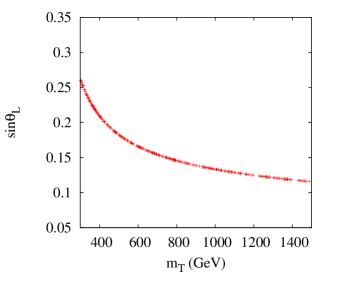
Figure 1: Upper limit at $95\%$ CL on the (left-handed) mixing angle as a function of the $T$ quark mass in the 2HDM-II with an up-like VLQ.

In general, when the new physics scale is much larger than the EW scale, virtual effects of the new particles in loops are expected to contribute to the EWPOs that have been precisely measured at LEP1, LEP2, SLC and Tevatron. These EWPOs are known as the oblique parameters $S,T$ and $U$ Peskin:1991sw and can be used to put constraints on new physics. In our case, the mixing between $t$-$T$ will generate couplings between the SM gauge bosons and the new VLQ, $T$, which will induce contributions to $S$ and $T$ Lavoura:1992np .

We have computed the extra contributions of the VLQ to $\Delta T=T-T_{\rm SM}$ and $\Delta S=S-S_{\rm SM}$ by implementing the model into the FeynArts Hahn:2000kx , FormCalc Hahn:1998yk ; FC-LT and LoopTools vanOldenborgh:1990yc ; LT packages, which are used to calculate the required gauge boson self-energies. In fact, in our case, the extra contribution to $\Delta\{T,S\}$ can be cast into pure 2HDM and VLQ parts, such that $\Delta\{T,S\}=\Delta\{T,S\}_{\rm 2HDM}+\Delta\{T,S\}_{\rm VLQ}$. In the present work, we focus on the decoupling limit where $m_{A}=m_{H}=m_{H^{\pm}}\gg m_{Z}$ and $\sin(\beta-\alpha)=1$, or slight departures from it, which leads to $\Delta T_{\rm 2HDM}=0$ and $\Delta S_{\rm 2HDM}=0$. We are then left only with the extra contribution of the VLQ. A straightforward calculation yields

$$\Delta T_{\rm VLQ} = \frac{3m^{2}_{t}s^{2}_{L}}{16m^{2}_{W}\pi(-1+r)s^{2}_{W}}\left((-1+r)(-2+(1+r)s^{2}_{L})-2rc^{2}_{L}\log r\right)\,\,\,{\rm with}\,\,\,r=\frac{m_{T}^{2}}{m_{t}^{2}},$$ (52)

$$\Delta S_{\rm VLQ} = \frac{1}{12m_{Z}^{2}\pi}\{-m_{t}^{2}s_{L}^{2}+m_{T}^{2}(s_{L}^{2}+32s_{W}^{2}c_{W}^{2})+s_{L}^{2}(m_{Z}^{2}(10-9s_{L}^{2})-6m_{t}^{2}c_{L}^{2}+6m_{T}^{2}c_{L}^{2})A_{0}[m_{t}^{2}]$$ (53)

$$+(s_{L}^{2}(6m_{t}^{2}c_{L}^{2}-6m_{T}^{2}c_{L}^{2}+m_{Z}^{2}(-10+9s_{L}^{2}))-32m_{Z}^{2}s_{W}^{2}c_{W}^{2})A_{0}(m_{T}^{2})$$

$$+3m_{t}^{2}s_{L}^{2}(10-3s_{L}^{2})B_{0}(0,m_{t}^{2},m_{t}^{2})-18m_{t}^{2}s_{L}^{2}c_{L}^{2}B_{0}(0,m_{t}^{2},m_{T}^{2})$$

$$-m_{T}^{2}(12s_{L}^{2}+9s_{L}^{4}-32s_{W}^{2}c_{W}^{2})B_{0}(0,m_{T}^{2},m_{T}^{2})$$

$$+2s_{L}^{2}(m_{Z}^{2}(2-3s_{L}^{2})+m_{t}^{2}(-14+3s_{L}^{2}))B_{0}[m_{Z}^{2},m_{t}^{2},m_{t}^{2}]$$

$$+6((m_{t}^{2}-m_{T}^{2})^{2}+(m_{t}^{2}+m_{T}^{2})m_{Z}^{2}-2m_{Z}^{4})s_{L}^{2}c_{L}^{2}B_{0}[m_{Z}^{2},m_{t}^{2},m_{T}^{2}]$$

$$+2s_{L}^{2}(m_{Z}^{2}(4-3s_{L}^{2})+m_{T}^{2}(8+3s_{L}^{2}))B_{0}[m_{Z}^{2},m_{T}^{2},m_{T}^{2}]\},$$

where the $A_{0}$ and $B_{0}$ functions are the standard Passarino-Veltman ones used in the convention of LoopTools LT . Note that our results agree numerically with Ref. Sally . Taking the above analytical expressions into account, our model will remain viable as long as $\Delta T_{\rm VLQ}$ and $\Delta S_{\rm VLQ}$ are compatible with the latest extracted values pdg which are given by

$$\Delta T=0.1\pm 0.07,\quad\quad\quad\Delta S=0.06\pm 0.09,$$ (54)

where a correlation coefficient $\rho=+0.91$ and $\Delta U=0$ have been used. We thus perform a random scan on the $s_{L}$ and $m_{T}$ parameters imposing compatibility with $\Delta T$ and $\Delta S$ at 95$\%$ CL, which yields a constraint on $s_{L}$ as a function of the VLQ mass, $m_{T}$, as shown in Fig. 1. One can see that the constraint on the mixing is, e.g., $|s_{L}|\leq 0.25$ for $m_{T}=350$ GeV and $|s_{L}|\leq 0.12$ for $m_{T}=1$ TeV. For a heavy VLQ, the constraint on the mixing is more severe and is mainly coming from $\Delta T$ which contains a large logarithm of $m_{T}^{2}/m_{t}^{2}$.

III.3 Constraints from $B\to X_{s}\gamma$

In addition to the EWPOs constraints studied above, the penguin induced $b\to s\gamma$ decay is also sensitive to new physics. The current experimental value is BR$(\bar{B}\to X_{s}\gamma)^{\rm exp}=(3.32\pm 0.15)\times 10^{-4}$, for $E_{\gamma}>1.6$ GeV Amhis:2016xyh , and the SM prediction with Next-to-Next-to-Leading Order (NNLO) QCD corrections is BR$(\bar{B}\to X_{s}\gamma)^{\rm SM}=(3.36\pm 0.23)\times 10^{-4}$ Czakon:2015exa ; Misiak:2015xwa . Since the SM result is close to the experimental data, $\bar{B}\to X_{s}\gamma$ will give a strict bound on new physics effects. The effective Hamiltonian arising from the $W^{\pm}$ and $H^{\pm}$ bosons for $b\to s\gamma$ at the $\mu_{b}=4.8$ GeV scale can be written as:

$${\cal H}_{b\to s\gamma}=-\frac{4G_{F}}{\sqrt{2}}\sum_{i=t,T}V^{*}_{is}V_{ib}\left(C^{i}_{7\gamma}(\mu_{b})O_{7\gamma}+C^{i}_{8\gamma}(\mu_{b})Q_{8G}\right)\,,$$ (55)

where the EM and gluonic dipole operators are given as:

$$O_{7\gamma}=\frac{e}{16\pi^{2}}m_{b}\bar{s}\sigma^{\mu\nu}P_{R}bF_{\mu\nu}\,,\ O_{8G}=\frac{g_{s}}{16\pi^{2}}m_{b}\bar{s}_{\alpha}\sigma^{\mu\nu}T^{a}_{\alpha\beta}P_{R}b_{\beta}G^{a}_{\mu\nu}\,.$$ (56)

Here, $C_{7\gamma}(\mu_{b})$ and $C_{8G}(\mu_{b})$ are the Wilson coefficients at the $\mu_{b}$ scale and their relations to the initial conditions at the high energy scale $\mu_{H}$ (needed to describe the evolution from such a high scale down to the lower energy $\mu_{b}$ via the matching scale $\mu_{0}$ Borzumati:1998tg ) are through Renormalization Group Equations (RGEs). The NLO Ciuchini:1997xe ; Borzumati:1998tg ; Borzumati:1998nx and NNLO Hermann:2012fc QCD corrections to $C_{7\gamma}(\mu_{b})$ and $C_{8G}(\mu_{b})$ in the 2HDM-II have been calculated. Based on the $C^{\rm SM}_{7\gamma}(\mu_{b})$ value extracted in Blanke:2011ry , we get $C^{\rm SM}_{7\gamma}(\mu_{b})\approx-0.310$ when BR$(\bar{B}\to X_{s}\gamma)^{\rm SM}=3.36\times 10^{-4}$ is applied. In order to study the influence of the $b\to s\gamma$ process on the 2HDM+VLQ model, we follow the approach in Misiak:2015xwa and split the BR$(\bar{B}\to X_{s}\gamma)$ as follows:

$${\rm BR}(\bar{B}\to X_{s}\gamma)\times 10^{4}\approx(3.36\pm 0.23)-8.22\,Re(C^{i}_{7\gamma})-1.99\,Re(C^{i}_{8G})\,,$$ (57)

where $C^{i}_{7\gamma,8G}$ are the Wilson coefficients at the $\mu_{H}=m_{H^{\pm}}$ scale (the matching scale is $\mu_{0}\sim m_{t}$ at which the heavy particles are decoupled Misiak:2015xwa ) , wherein the quadratic $C^{i}_{7\gamma,8G}$ terms are ignored due to the requirement of $C^{i}_{7\gamma,8G}<1$. Using the current experimental value, the bound on $C^{i}_{7\gamma,8G}$ is:

$$8.22Re(C^{i}_{7\gamma})+1.99Re(C^{i}_{8G})\approx 0.04\pm 0.28.$$ (58)

According to the charged Higgs interactions, the $H^{\pm}$ contributions coming together with $t$ and $T$ to $C^{i}_{7\gamma,8G}$ are expressed as Borzumati:1998tg :

$$C^{i}_{7\gamma} =f_{1\gamma}(x_{i})/\tan^{2}\beta+f_{2\gamma}(x_{i})\,,$$

$$C^{i}_{8G} =f_{1G}(x_{i})/\tan^{2}\beta+f_{2G}(x_{i}),$$ (59)

with $x_{i}=m^{2}_{i}/m^{2}_{H^{\pm}}$ and $i=t,T$. The form factors are given in Appendix B.

Fig. 2 shows the limits on $V_{Tb}$ (left) and $m_{H^{\pm}}$ (right) in the 2HDM+VLQ. We learn that BR$(b\to s\gamma)$ excludes $V_{Tb}\geq 0.03$ regardless of the value of $m_{T}$ used. It further appears from the right panel of Fig. 2 that large $\tan\beta$ is not excluded by current data and a lower bound $m_{H^{\pm}}\geq$ 600 GeV is obtained similar to the case of the standard 2HDM-II, (Recall that a lower bound $m_{H^{\pm}}\geq$ 580 GeV was obtained in Misiak:2017bgg for this case.)

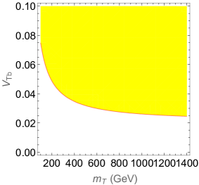
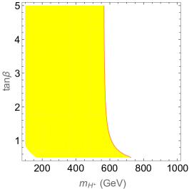
Figure 2: Excluded regions (yellow color) at $95\%$ CL from BR($\bar{B}\to X_{s}\gamma$) in the 2HDM+VLQ. Left panel: Limit on $V_{Tb}$ as a function of $m_{T}$ with $m_{H^{\pm}}=600$ GeV. Right panel: Limit on the charged Higgs mass with $m_{T}=400$ GeV and $V_{Tb}=0.025$.

III.4 Constraints from LHC data

The couplings of the SM-like Higgs are sensitive to the parameters $\cos(\beta-\alpha)$ and $\tan\beta$. Therefore, the LHC data on the 125 GeV Higgs boson can give strong constraints on these. In Fig. 3, we show the constraints on the ordinary 2HDM (left) and 2HDM+VLQ (right) using Higgs data from Run 1 (gray) and Run 2 (yellow) at 95$\%$ CL. The bounds on $\cos(\beta-\alpha)$ are much more stringent for the ordinary 2HDM-II, where the SM-like coupling region of the 125 GeV Higgs forces $|\cos(\beta-\alpha)|<0.14$, and increasingly more stringent for larger $\tan\beta$. However, in the so-called ‘wrong sign’ Yukawa coupling region of the 125 GeV Higgs state, we find $|\cos(\beta-\alpha)|<0.45$. By varying $|s_{L}|<0.20$ and 400 GeV$<m_{T}<$ 1000 GeV and setting $y_{T}=4\pi$, the situation in the 2HDM+VLQ (right panel) is quite different for low $\tan\beta$, where $|\cos(\beta-\alpha)|<0.4$.

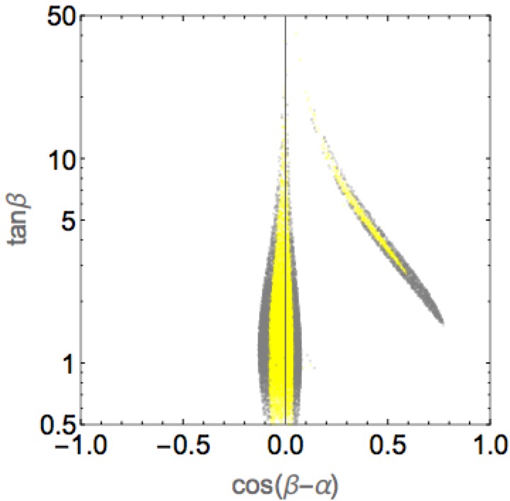
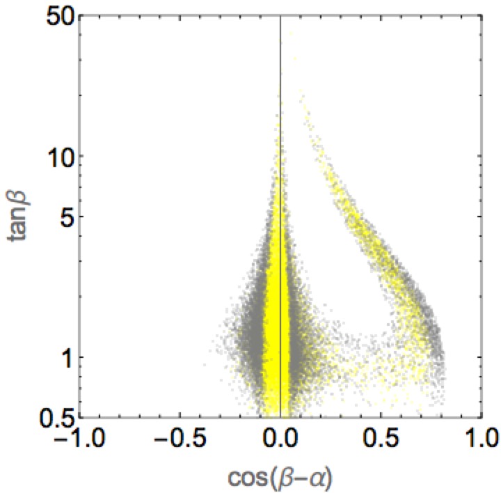
Figure 3: Constraints from the LHC Higgs data on the parameter space of the ordinary 2HDM (left) and 2HDM+VLQ (right). We show the 95$\%$ CL region in the $(\cos(\beta-\alpha),\tan\beta)$ plane. The gray (yellow) regions were obtained using Higgs Run 1(2) data. We have varied $|s_{L}|<0.20$ and 400 GeV$<m_{T}<$ 1000 GeV and set $y_{T}=4\pi$.

Another constraint, this time on the mixing, $s_{L}$, comes from the contribution of the VLQ to the di-photon event rate of the $\approx 125$ GeV SM-like Higgs boson. The modified top quark coupling to this Higgs boson and the presence of an additional heavy quark can impact loop induced Higgs decays, namely, $h\to gg$, $h\to\gamma\gamma$ and $h\to Z\gamma$. The relevant partial decay widths are given by

$$\Gamma(\phi\to\gamma\gamma) = \frac{G_{F}\alpha^{2}m^{3}_{\phi}}{128\sqrt{2}\pi^{3}}\left|\frac{4}{3}\sum_{f=t,T}\kappa^{\phi}_{ff}A^{\phi}_{1/2}(\tau_{f})+\kappa^{\phi}_{WW}A^{\phi}_{1}(\tau_{W})+g^{\phi}_{H^{\pm}H^{\mp}}\frac{m^{2}_{W}}{2c^{2}_{W}m^{2}_{H^{\pm}}}A^{\phi}_{0}(\tau_{H^{\pm}})\right|^{2},~{}~{}~{}$$ (60)

$$\Gamma(\phi\to Z\gamma) = \frac{G^{2}_{F}m^{2}_{W}\alpha m^{3}_{\phi}}{64\pi^{4}}\left(1-\frac{m^{2}_{Z}}{m^{2}_{\phi}}\right)^{3}\Bigg{|}\sum_{f=t,T}\kappa^{\phi}_{ff}\frac{2n_{f}Q_{f}(I^{3}_{f}-2s^{2}_{W}Q_{f})}{c_{W}}A^{\phi}_{1/2}(\tau_{f},\lambda_{f})$$

$$+ \sum_{f,f^{\prime}=t,T}\frac{m_{f(f^{\prime})}}{m_{W}}\sum_{m=L,R}\kappa^{\phi}_{ff^{\prime}}g^{m}_{ff^{\prime}}A^{\phi}_{1/2}(\tau_{f},\lambda_{f^{\prime}})+\kappa^{\phi}_{WW}A^{\phi}_{1}(\tau_{W})+g^{\phi}_{H^{\pm}H^{\mp}}\frac{m^{2}_{W}}{m^{2}_{H^{\pm}}}\frac{c_{2W}}{c_{W}}A^{\phi}_{0}(\tau_{H^{\pm}})\Bigg{|}^{2}$$

$$\Gamma(A\to\gamma\gamma) = \frac{G_{F}\alpha^{2}m^{3}_{A}}{128\sqrt{2}\pi^{3}}\left|\frac{4}{3}\sum_{f=t,T}\kappa^{A}_{ff}A^{A}_{1/2}(\tau_{f})\right|^{2},$$ (62)

$$\Gamma(A\to Z\gamma) = \frac{G^{2}_{F}m^{2}_{W}\alpha m^{3}_{A}}{16\pi^{4}}\left(1-\frac{m^{2}_{Z}}{m^{2}_{A}}\right)^{3}$$

$$\Bigg{|}\sum_{f=t,T}\kappa^{A}_{ff}\frac{2n_{f}Q_{f}(I^{3}_{f}-2s^{2}_{W}Q_{f})}{c_{W}}A^{A}_{1/2}(\tau_{f},\lambda_{f})+\sum_{f,f^{\prime}=t,T}\frac{m_{f(f^{\prime})}}{m_{W}}\sum_{m=L,R}\kappa^{A}_{ff^{\prime}}g^{m}_{ff^{\prime}}A^{A}_{1/2}(\tau_{f},\lambda_{f^{\prime}}))\Bigg{|}^{2},$$

where $\phi=h(\equiv h_{\rm SM}$) or $H$ are the CP-even Higgs bosons of the 2HDM, with $\kappa^{h(H)}_{WW}=\sin(\beta-\alpha)(\cos(\beta-\alpha))$. The relevant loop functions can be found in, e.g., Refs. Spira:1997dg ; Djouadi:2005gi . Clearly, the charged Higgs boson contributions are smaller compared to the fermionic ones. Even for large $g_{\phi H^{\pm}H^{\mp}}$, the charged Higgs effects are still negligible, henceforth, we neglect these.

The relevant modifications to the signal strength $\mu^{h}_{\gamma\gamma}$ (a function of the production cross-sections and decay BRs) are defined in our scenario as

$$\mu^{h}_{V\gamma}\equiv\frac{\sigma^{\rm VLQ}(pp\to\phi)}{\sigma(pp\to h_{\rm SM})}\times\frac{{\rm BR}^{\rm VLQ}(\phi\to V\gamma)}{{\rm BR}(h_{\rm SM}\to V\gamma)},\quad\quad V=Z,\gamma,\quad\phi=H,A~{}(\rm{summed~{}over}).$$ (63)

These come from the presence of an additional VLQ in the loops as well as from the modification of the $ht\bar{t}$ coupling for both Higgs production ($gg\to\phi$) and Higgs decay ($\phi\to V\gamma$). The theoretical value for $\mu^{h}_{\gamma\gamma}$ will depend on $m_{T}$, $s_{L}$ as well as the new Yukawa $y_{T}$. However, in the decoupling limit $\cos(\beta-\alpha)=0$, the dependence of $ht\bar{t}$ and $hT\bar{T}$ on $y_{T}$ cancels due to a factor $\cos(\beta-\alpha)=0$. What then remains is solely an $m_{T}$ and $s_{L}$ dependence, at least in the $V=\gamma$ case. The formula in Eq. (63) holds for the $Z\gamma$ case as well, wherein, however, the role of the $T$ loops can be altered significantly relative to that of the others by the additional degree of freedom carried by the $ZT\bar{T}$ vertex (unlike the case of the $\gamma T\bar{T}$ one, which is fixed by the Ward identity). Further, unlike the case of $\gamma\gamma$, $Z\gamma$ also benefits from non-diagonal loop transitions wherein the vertices $H,At\bar{T}$ and $Zt\bar{T}$ (and c.c.) are involved. These differences between the two decay channels will play a key role in the remainder of our analysis.

The effects of a new heavy quark, $T$, have direct consequences for the signal strengths of the SM-like Higgs boson. In Fig. 4, we illustrate a contour plot for $\mu^{h}_{\gamma\gamma}$ over the ($s_{L}$, $y_{T}$) plane. The dashed black, solid black and solid red contours capture $\mu^{h}_{Z\gamma}=1$, 1.5 and 2, respectively. The three contours fall within 1$\sigma$ of the ATLAS and CMS measured value of $\mu^{h}_{\gamma\gamma}=1.10\pm 0.23~{}({\rm stat})\pm 0.22~{}({\rm syst})$. One can therefore conclude that this LHC constraint is less stringent than the oblique parameters previously discussed. However, once the $\mu^{h}_{\gamma\gamma}$ measurement improves with Run 2 data from the LHC and reaches the level of 10% or less deviation from the SM value, then the $\approx 125$ GeV di-photon event constraints will be more stringent. The pattern of $\mu^{h}_{Z\gamma}$ is also given. It is remarkable that, for $\mu^{h}_{\gamma\gamma}$ compatible with LHC data at the $\pm 2\sigma$ level, $\mu^{h}_{Z\gamma}$ can see an enhancement up to a factor of nearly 2.

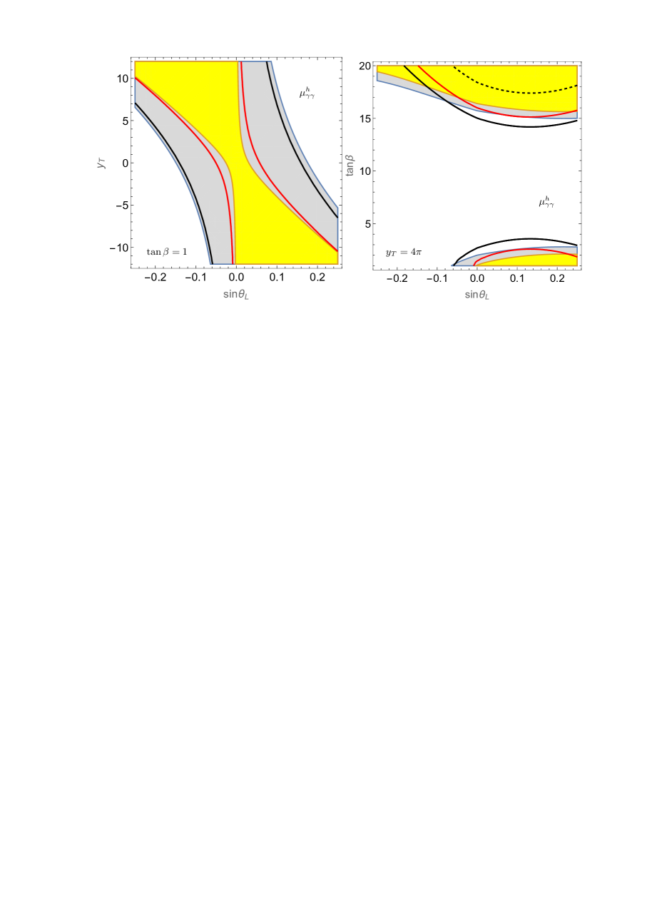
Figure 4: Allowed regions for $\mu^{h}_{\gamma\gamma}$ in the 2HDM+VLQ at 95$\%$CL of Higgs data Run 1 (gray) and Run 2 (yellow) over the ($s_{L},y_{T}$) plane (left) with $\tan\beta=1$ and over the ($s_{L},\tan\beta$) plane (right) with $y_{T}=4\pi$. The other parameters are fixed to $m_{T}=1$ TeV, $\cos(\beta-\alpha)=0.05$. The contour plots correspond to $\mu^{h}_{Z\gamma}=1$ (dashed black), 1.5 (solid red) and 2 (solid black).

IV Confronting the 2HDM+VLQ with LHC data

In order to explain the LHC data in the framework of our 2HDM+VLQ construct, we consider the $gg\to\phi$ and $\phi\to\gamma\gamma$ (with $\phi=H$ and $A$) processes where the contribution of all the quarks including $T$ is considered. In the SM, only the top-quark loop gives a significant fermionic contribution. Besides the top-quark, the new VLQ state $T$ can also contribute in the 2HDM+VLQ case, for both the SM-like and the other heavy Higgs production modes in addition to their decays into di-photons.

We start by assuming that we are in the alignment limit of the light Higgs boson $h$, $\cos(\beta-\alpha)=0$, wherein the heavier CP-even Higgs boson, $H$, decays to $W^{+}W^{-}$ and $ZZ$ vanish at the tree level, which is consistent with current Higgs boson searches. (Needless to say, the $A$ state cannot directly couple to pairs of SM massive gauge bosons in presence of CP conservation). We also assume that the heavy Higgs states are degenerate, $m_{H}=m_{A}$, which is favored by satisfying theoretical bounds such as vacuum stability, perturbativity and allowed by EWPOs Olive:2016xmw .

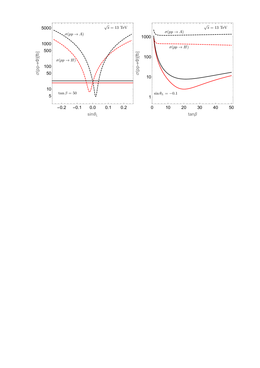
Figure 5: Heavy Higgs production $\sigma(pp\to A,H)$ in fb at the LHC with $\sqrt{s}=13$ TeV as a function of $\sin\theta_{L}$ (left) and $\tan\beta$ (right) for $m_{H}=m_{A}=700$ GeV in the alignment limit of the 2HDM+VLQ. We fix $y_{T}=2\pi$, $m_{T}=700$ GeV and $\cos(\beta-\alpha)=0$. The solid (black and red) lines correspond to 2HDM without VLQ.

The cross-section for this process is given by

$$\sigma^{\rm VLQ}(pp\to\phi)=\sigma(pp\to h_{\rm SM})\times\frac{\Gamma^{\rm VLQ}(\phi\to gg)}{\Gamma(h_{\rm SM}\to gg)},\quad\quad\phi=H,A,$$ (64)

where $\Gamma^{\rm VLQ}(\phi\to gg)$ is the $gg$ width of the SM augmented by the extra VLQ loop contribution. The SM Higgs cross-section is taken from the Higgs working group study of Ref. HWG . In our 2HDM+VLQ scenario, the cross-section can be enhanced from the additional VLQ loop, which introduces the $hT\bar{T}$ coupling which can be large. Its sign is such that it can enable constructive interference with the top quark loop. Furthermore, the BR${}^{\rm VLQ}(H,A\to\gamma\gamma)$ can overall be enhanced as well through a similar dynamics, though it should be recalled here that the dominant loop is due to $W^{\pm}$’s which typically have an opposite sign to the $t$ and $T$ loops, owing to the different spin statistics. In Fig. 5, fixing $m_{H}=m_{A}=700$ GeV, we present the dependence of $\sigma(pp\to H,A)$ upon $s_{L}$ for $\tan\beta=50$ while the right panel shows the same quantity as a function of $\tan\beta$ with fixed mixing angle $s_{L}=-0.1$. Both panels are for a large Yukawa of the new top, $y_{T}=2\pi$ with $m_{T}=700$ GeV. Here, $\tan\beta$ is required to be smaller than 20 for $m_{H}=m_{A}=700$ GeV. It is clear from Fig. 5 that, away from the $s_{L}\approx 0$ limit (left frame), the $pp\to H,A$ process can differ by two orders of magnitude compared to the ordinary 2HDM-II.

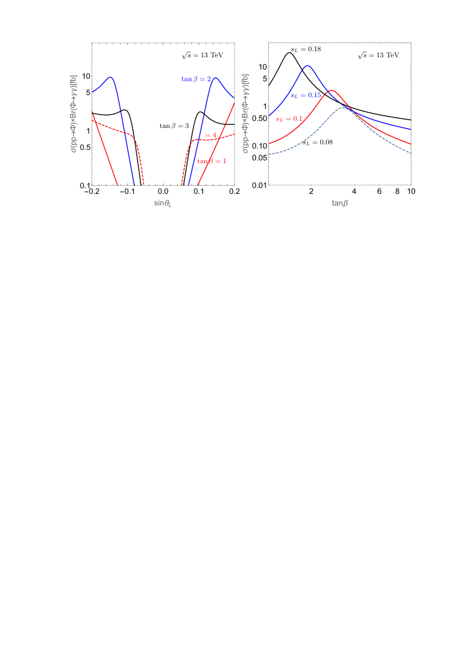
Figure 6: Cross sections of $(pp\to H,A\to\gamma\gamma)$ in fb in the 2HDM+VLQ as a function of $s_{L}$ for different values of $\tan\beta$ (left) and $\tan\beta$ for different values of $s_{L}$ (right). Here, $\cos(\beta-\alpha)=0$, $m_{H}=m_{A}=700$ GeV, $m_{T}=700$ GeV and $y_{T}=4\pi$.

In the left panel of Fig. 6 we present the dependence of $\sigma(pp\to\phi)\times{\rm BR}(\phi\to\gamma\gamma)$ upon the mixing angle $s_{L}$ for $\tan\beta=1,2,3,4$ while the right panel shows the same quantity as a function of $\tan\beta$ with fixed mixing angles $s_{L}$. Both panels are for a large Yukawa of the new top, $y_{T}=4\pi$. In this illustration, we limit ourselves to low $\tan\beta$ values which are favored by $\tau\tau$ LHC data and also because of perturbative unitarity coming from the 2HDM scalar potential. We emphasize that, in the decoupling limit which we consider, the $W^{\pm}$ loop in $H\to\gamma\gamma$ vanishes since it is proportional to $\cos(\beta-\alpha)\approx 0$ while $A\to\gamma\gamma$ has no $W^{\pm}$ loop at all because of the CP-odd nature of the $A$ state. Furthermore, for $H,A\to gg$, we are only left with top quarks and VLQ contributions. It is clear from Fig. 6 that, away from the $s_{L}\approx 0$ limit (left frame), the $pp\to H,A\to\gamma\gamma$ process can significantly contribute to the high mass di-photon event sample. Hence, the recent studies carried out by ATLAS and CMS have the potential to significantly constrain our model. For example, for $H,A$ masses around 500 GeV, $\tan\beta$ values of 2–3 are not possible, as no particular feature has emerged from the LHC data in the relevant $m_{\gamma\gamma}$ invariant mass range (hence they are compatible with the SM rates, driven by $q\bar{q},gg\to\gamma\gamma$ events). In fact, the strongest constraints would emerge (right frame) for any $m_{A}=m_{H}$ value whenever a loop threshold opens up, whether this is the $t\bar{t}$ one at 350 GeV or the $T\bar{T}$ one at higher energies (possibly excluding $\tan\beta\approx 4$ values), which may happen through both Higgs HHG and $Z$ Moretti:2014rka ; Jain:2016rhk boson mediation.

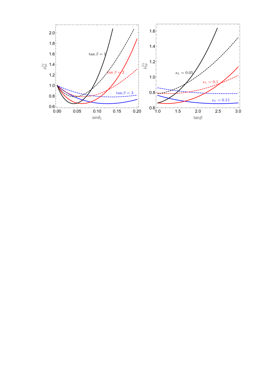
Figure 7: Ratios of $\sigma(gg\to H,A\to\gamma\gamma)$ (solid) and $\sigma(gg\to H,A\to Z\gamma)$ (dashed) in the 2HDM+VLQ over the 2HDM for $m_{\gamma\gamma}=m_{Z\gamma}=750$ GeV as a function of $s_{L}$ for different values of $\tan\beta$ (left) and Yukawa coupling $y_{T}$ (right). Here, $\cos(\beta-\alpha)=0$, $m_{H}=m_{A}=700$ GeV, $m_{T}=700$ GeV. Also, we fix, $y_{T}=-2\pi$.

A point we have previously made regarding our 2HDM+VLQ construct is the possibility of $\gamma\gamma$ rates at high invariant masses being compatible with Run 2 data with the $Z\gamma$ ones being potentially different from the standard 2HDM-II case. With this in mind, we present Fig. 7, where the inclusive rates of these two channels in the 2HDM+VLQ are shown, divided by the corresponding 2HDM rates (these correspond to the case of $s_{L}=0$ and $m_{T}\to\infty$), i.e.,

$$\mu^{V\gamma}_{pp}\equiv\frac{\sigma(gg\to H,A\to V\gamma)_{\rm 2HDM+VLQ}}{\sigma(gg\to H,A\to V\gamma)_{\rm 2HDM}},~{}~{}~{}~{}V=Z,\gamma,$$ (65)

for low $\tan\beta$ and negative $y_{T}$. It is clear that substantial differences (up to a factor of two) can exist between the two scenarios, so long that $s_{L}$ is sizably different from zero. (Local maxima in the plot correspond to relative sign changes between the VLQ loop contributions and the 2HDM ones). In fact, over most of the possible $s_{L}$ interval, both $\gamma\gamma$ and $Z\gamma$ in the 2HDM+VLQ depart simultaneously from the ordinary 2HDM-II case.

As pointed out in the introduction, ATLAS and CMS have reported a possible increase in the signal strength of the $t\bar{t}h$ associated production mode in the LHC data. The most recent preliminary results from Run 2 relayed by CMS still show an enhancement of $\mu^{pp}_{t\bar{t}h}$ = 1.5 $\pm$ 0.5 times the SM prediction with an observed significance of 3.3$\sigma$ compared to the expected one of 2.5$\sigma$ (obtained from combining results of Run 1). Many different final states contribute to this enhancement, but the most significant excesses are observed in multi-lepton final states which probe closely $t\bar{t}h$ production. One possibility to explain the excess is that it could be due to the modified Higgs coupling to the SM top quark, resulting in an enhanced $t\bar{t}h$ production. Mixing within the top sector, i.e., between the $t$ and $T$ states, also allows for a sufficiently large enhancement of the $pp\to t\bar{t}h$ rates. Hence, a possibility offered by our scenario could be the potential to explain a $t\bar{t}h$ enhancement. In this case, rates for the loop-induced processes of the $h$ should remain SM-like, despite the VLQ contributions in our scenario.

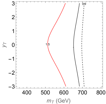
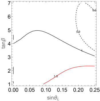
Figure 8: Contour plots for the Higgs signal strength $\mu^{pp}_{t\bar{t}h}$ over the ($\sin\theta_{L}$, $\tan\beta$) plane (right) and over the ($m_{T}$, $y_{T}$) plane (left) in the 2HDM+VLQ with $\cos(\beta-\alpha)=0$, $m_{h}=125.5$ GeV, $m_{H}=m_{A}=m_{H^{\pm}}=600$ GeV for ($\sin\theta_{L}$, $\tan\beta$)=(0.22, 1.5) in the left panel and ($m_{T}$, $y_{T}$)=(400 GeV, 2) in the right panel, at the LHC Run 2. In both plots the red line corresponds to $\mu^{pp}_{t\bar{t}h}=1.5$, the solid black one to $\mu^{pp}_{t\bar{t}h}=1$ and the dashed black one to $\mu^{pp}_{t\bar{t}h}=0.9$.

In Fig. 8 we show contour plots of $\mu^{pp}_{t\bar{t}h}$ in the ($\sin\theta_{L}$, $\tan\beta$) plane (right) and ($m_{T}$, $y_{T}$) plane (left) in the 2HDM+VLQ given SM-like Higgs couplings. As can be seen from the figure, there is a strong dependence upon both the parameters $\sin\theta_{L}$ and $\tan\beta$. Clearly, the 2HDM+VLQ can reproduce a higher value of the $t\bar{t}h$ signal strength than in the SM, typically $\mu^{pp}_{t\bar{t}h}\approx 1.5$, for small $\tan\beta$ and $\sin\theta_{L}=0.22$, i.e., a parameter space configuration ideally testable within the experimental range of LHC Run 2 through direct $T$ production.

In fact, in the light of a possible explanation of potentially anomalous $t\bar{t}h$ data afforded by a heavy top with $m_{T}\approx 600$ GeV, we end this section with a few comments on the possible production and decay patterns for such a VLQ state, as the ensuing signatures would be a distinctive feature between a standard 2HDM-II and its VLQ version. Unlike the case of the SM+VLQ framework where the BR of $T\to bW^{+}$, $T\to tZ$ and $T\to th$ are, respectively, 50%, 25% and 25% for heavy $m_{T}$, in models with more than one Higgs doublet, several decay patterns can appear from the interaction of the new heavy quark with the extended Higgs sector, e.g.,

$$T\quad\to\quad bW^{+},\quad tZ,\quad th,\quad tH,\quad tA,\quad bH^{+},$$ (66)

where the last three cases are unique to a 2HDM sector. (The partial widths for all these modes are given in Appendix C).

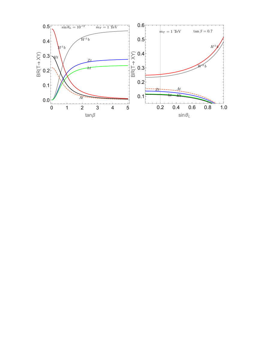
Figure 9: Branching ratios of $T$ in the 2HDM+VLQ as a function of $\tan\beta$ (left) and a a function of $\sin\theta_{L}$ (right) with $y_{T}=2$, $m_{h}=125.5$ GeV, $m_{A}=m_{H}=500$ GeV, $m_{H^{\pm}}=600$ GeV, $\cos(\beta-\alpha)=0$, $m_{T}=1$ TeV with $\tan\beta=0.7$ (right) and $\sin\theta_{L}=V_{Tb}=10^{-2}$ (left).

In Fig. 9 we illustrate the BRs of the $T$ quark as a function of $\sin\theta_{L}$ (right panel) and as a function of $\tan\beta$ (left panel). We assume a heavy scalar scenario where $m_{H}=m_{A}=500$ GeV, $H^{\pm}=600$ GeV and $m_{T}=1$ TeV. As seen from the right plot for $\tan\beta=0.7$, $T\to bW^{+}$ and $T\to bH^{+}$ are comparable and could reach 25$\%$ at small mixing $\sin\theta_{L}=0$ instead of 50$\%$ in the SM for $T\to bW^{+}$. However, $T\to th$ and $tZ$ are slightly smaller compared to SM+VLQ case (less than 12%). a function of $\tan\beta$ and with small mixing $\sin\theta_{L}=10^{-2}$. We see that in the limit $\sin\theta_{L}\to 0$, when the non-standard $T$ decay modes $T\to tH,tA$ are suppressed due to their coupling, which is proportional to $\sin\theta_{L}$, $T\to bH^{+}$ is comparable to $T\to bW^{+}$ for $\tan\beta\approx 0.5-0.7$ and may offer an alternative discovery mode. We stress here that $b\to s\gamma$ constraint is fulfilled for such small $\tan\beta\approx 0.5-0.7$ if $m_{H^{\pm}}=600$ GeV.

Finally, in Fig. 10 (left) we illustrate the branching fractions of the heavy top as a function of $m_{T}$. As it can be seen, when non-SM decays such as $T\to bH^{+},tH,tA$ are not open, the situation is similar to the SM+VLQ case, as expected. However, when $T\to bH^{+},tH,tA$ are open, one can see that $T\to bH^{+}$ compete with $T\to bW^{+}$ and even dominate for high $m_{T}$. Note that, at large $m_{T}$, $T\to tH,tA$ are slightly larger than the SM decays $T\to th,tZ$.

There exist several LHC analyses searching for (model-independent) pair produced new VLQ states, performed by both ATLAS and CMS. These place limits in the range 600–800 GeV depending on the actual BR of the $T$ quark in the channels searched for. These do not presently include the $T\to bH^{+}$ mode. However, with $m_{T}=1000$ GeV, the $T\bar{T}\to b\bar{b}H^{+}H^{-}$ mode (followed by $H^{+}H^{-}\to b\bar{b}b\bar{b}W^{+}W^{-}$ decays) can lead to ‘$W^{+}W^{-}$ plus $6b$-jets’ as a sizeable and (very distinctive) signature. Even with small $\sin\theta_{L}$, an interesting possibility would be $T\bar{T}\to b\bar{b}W^{+}H^{-}$ decays, with $H^{-}\to b\bar{b}W^{-}$, producing an equally distinctive ‘$W^{+}W^{-}$ plus $4b$-jets’ signal. While also the ‘$W^{+*}W^{-*}W^{+}W^{-}$ plus $4b$-jets’ case is a potentially interesting channel, stemming from $T\bar{T}\to t\bar{t}hh\to b\bar{b}W^{+}W^{-}hh$ with $hh\to b\bar{b}W^{+*}W^{-*}$ decays, given that $T\to th$ is probably very difficult to detect (as intimated already, see Harigaya:2012ir ), the alternative of accessing the new VLQ state via $T\to bH^{+}$ decays becomes a very intriguing one. In fact, this is the ideal channel to characterize our model, as even neutral $A,H$ decays are, so-to-say, ‘degenerate’ (i.e., they can have the same decay patterns) with those from the SM-like Higgs state, $h$. Needless to say, to establish this signature would represent circumstantial evidence of a 2HDM+VLQ structure. Typical $H^{\pm}$ decay patterns can be found in Fig. 10 (right), showing that $b\bar{b}W^{\pm}$ decays of a charged Higgs bosons (via $tb,W^{\pm}A$) are indeed the dominant ones for large $m_{H^{\pm}}$ values.

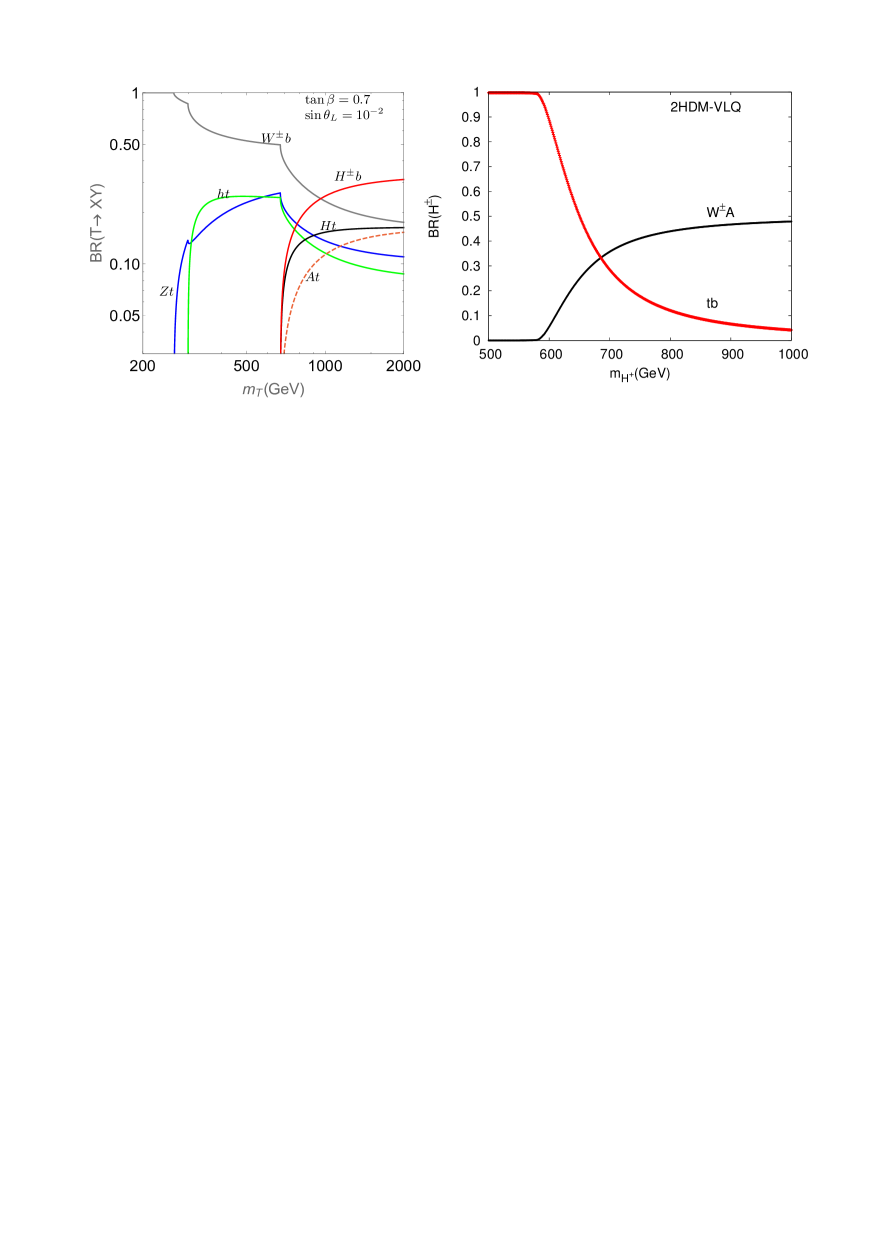
Figure 10: Left: BRs of the $T$ as a fucntion of $m_{T}$ with the same parameter as in Fig. 9. Right: BRs of the $H^{\pm}$ state in the 2HDM+VLQ as a function of its mass for $\sin\theta_{L}=0$, $y_{T}=6$, $m_{h}=125.5$ GeV, $m_{A}=m_{H}=500$ GeV, $\cos(\beta-\alpha)=0$, $\tan\beta=0.7$ and $m_{T}=1000$ GeV. (Here, we assume $m_{T}>m_{H^{\pm}}$, so that 2HDM-like decays only are included, i.e., the $H^{\pm}$ state cannot decay into final states with $T$s.)

V Conclusions

In this paper, we have extended the ordinary 2HDM-II by a singlet heavy VLQ with the same EM charge as the top quark. In the (near) decoupling limit of the 2HDM-II, one neutral CP-even Higgs state, $h$, can mimic the SM-like Higgs boson seen at the LHC Run 1 at $\approx 125$ GeV while the other two neutral Higgs states, $H$ and $A$, can be constrained as the model has to accommodate the data observed by ATLAS and CMS at the LHC Run 2 in both the low and high mass region, which are to date consistent with SM expectations. We have then proceeded to a phenomenological comparison between the 2HDM+VLQ scenario and the ordinary 2HDM case, limitedly to the LHC environment.

We have illustrated that a different decay pattern emerges in the 2HDM+VLQ with respect to the standard 2HDM when $\gamma\gamma$ and $Z\gamma$ samples are compared to each other. Then, we have shown that, at the same time, an enhancement of $\sigma(pp\to t\bar{t}h)$ by a factor up to 2 can occur, which would explain an increased value of such a cross-section at the LHC, i.e., in the direction of a possible enhancement seen in Run 2 data. All this can occur for VLQ masses of order 600–800 GeV, so that we have finally highlighted that non-SM-like decays of this VLQ state, particularly via $H^{\pm}$ channels, would be evidence of a 2HDM sector.

In fact, by combining these instances, a peculiar ‘smoking-gun’ situation may emerge in the 2HDM+VLQ scenario discussed here, where one has $\gamma\gamma$ rates at large invariant masses essentially compatible with the SM background, yet a depletion (with respect to the 2HDM yield) can be seen in the $Z\gamma$ sample, with or without an enhancement of the $t\bar{t}h$ cross-section. One could indeed disentangle this as being due to this particular BSM structure by finally revealing a variety of $T\to bH^{+}$ decays emerging from QCD induced $T\bar{T}$ production.

Remarkably, all such phenomenology can be obtained for parameter space configurations compliant with current theoretical and experimental constraints, as we have scrupulously assessed using up-to-date tools, yet ameanable to prompt phenomenological investigation in the upcoming years at the LHC, during Run 2 and 3.

Appendix A Yukawa couplings in the 2HDM+VLQ

These are as follows:

$$\kappa^{h}_{t\bar{t}} = c_{L}c_{R}(y^{h}_{t})-s_{R}c_{L}\left(c_{\beta\alpha}\frac{y_{T}}{y_{t}}+s_{\beta\alpha}\frac{\xi_{T}}{y_{t}}\right),$$ (67)

$$\kappa^{h}_{T\bar{T}} = s_{L}s_{R}(y^{h}_{t})+s_{L}c_{R}\left(c_{\beta\alpha}\frac{y_{T}}{y_{t}}+s_{\beta\alpha}\frac{\xi_{T}}{y_{t}}\right),$$ (68)

$$\kappa^{h}_{t\bar{T}} = c_{R}s_{L}(y^{h}_{t})-s_{R}s_{L}\left(c_{\beta\alpha}\frac{y_{T}}{y_{t}}+s_{\beta\alpha}\frac{\xi_{T}}{y_{t}}\right),$$ (69)

$$\kappa^{H}_{t\bar{t}} = c_{L}c_{R}(y^{H}_{t})+s_{R}c_{L}\left(s_{\beta\alpha}\frac{y_{T}}{y_{t}}-c_{\beta\alpha}\frac{\xi_{T}}{y_{t}}\right),$$ (70)

$$\kappa^{H}_{T\bar{T}} = s_{L}s_{R}(y^{H}_{t})-s_{L}c_{R}\left(s_{\beta\alpha}\frac{y_{T}}{y_{t}}-c_{\beta\alpha}\frac{\xi_{T}}{y_{t}}\right),$$ (71)

$$\kappa^{H}_{t\bar{T}} = c_{R}s_{L}(y^{H}_{t})+s_{R}s_{L}\left(s_{\beta\alpha}\frac{y_{T}}{y_{t}}-c_{\beta\alpha}\frac{\xi_{T}}{y_{t}}\right),$$ (72)

$$\kappa^{A}_{t\bar{t}} = i\left(c_{L}c_{R}(y^{A}_{t})+s_{R}c_{L}\frac{y_{T}}{y_{t}}\right),$$ (73)

$$\kappa^{A}_{T\bar{T}} = i\left(s_{L}s_{R}(y^{A}_{t})-s_{L}c_{R}\frac{y_{T}}{y_{t}}\right),$$ (74)

$$\kappa^{A}_{t\bar{T}} = i\left(s_{L}c_{R}(y^{A}_{t})+s_{R}s_{L}\frac{y_{T}}{y_{t}}\right).$$ (75)

The above reduced Higgs couplings $\kappa^{\phi}_{ij}$ are expressed in terms of the normalized $y^{\phi}_{t}$ ones given by

$$y^{h}_{t} = \sin(\beta-\alpha)+\cot\beta\cos(\beta-\alpha),$$

$$y^{H}_{t} = \cos(\beta-\alpha)-\cot\beta\sin(\beta-\alpha),$$

$$y^{A}_{t} = \cot\beta.$$ (76)

It is easy to check that, in the case of zero mixing $s_{L}=0$, the $\{h,H,A\}t\bar{t}$ couplings reduce to the 2HDM ones while $\{h,H,A\}t\bar{T}$ and $\{h,H,A\}T\bar{T}$ all vanish.

Appendix B Form factors for $b\to s\gamma$

These were used as follows:

$$f_{1\gamma}(x) =\frac{x}{72}\left[\frac{8x^{2}+5x-7}{(1-x)^{3}}-\frac{6x(2-3x)}{(1-x)^{4}}\ln(x)\right]\,,$$

$$f_{1G}(x) =\frac{x}{24}\left[\frac{x^{2}-5x-2}{(1-x)^{3}}-\frac{6x}{(1-x)^{4}}\ln(x)\right]\,,$$

$$f_{2\gamma}(x) =\frac{x}{12}\left[\frac{3-5x}{(1-x)^{2}}+\frac{2(2-3x)}{(1-x)^{3}}\ln(x)\right]\,,$$

$$f_{2G}(x) =\frac{x}{4}\left[\frac{3-x}{(1-x)^{2}}+\frac{2}{(1-x)^{3}}\ln(x)\right]\,.$$ (77)

Appendix C Partial widths of the VLQ

In this appendix we give the analytic expressions of the partial widths of the VLQ into vector and Higgs bosons, $T\to qV$ and $T\to q\phi$, as

$$\Gamma(T\to qV) = \frac{g^{2}}{32\pi}\frac{\beta}{m^{2}_{T}}\left((g^{2}_{L}+g^{2}_{R})\left(\frac{m^{2}_{T}+m^{2}_{q}}{2}+\frac{(m^{2}_{T}-m^{2}_{q})^{2}}{2m^{2}_{V}}-m^{2}_{V}\right)-6g_{L}g_{R}m_{T}m_{q}\right),$$ (78)

$$\Gamma(T\to q\phi) = \frac{\beta}{8\pi m^{2}_{T}}\left((g^{2}_{L}+g^{2}_{R})\frac{m^{2}_{T}+m^{2}_{q}-m^{2}_{\phi}}{2}+g_{L}g_{R}m_{T}m_{q}\right),$$ (79)

with

$$\beta=\frac{\left((m^{2}_{T}-(m_{q}+m_{X})^{2})(m^{2}_{T}-(m_{q}-m_{X})^{2})\right)^{p}}{2m_{T}}\quad\quad(X=V,\phi),$$ (80)

where $m_{V}$($m_{\phi}$) and $m_{q}$ are the masses of the gauge(Higgs) bosons and the SM quark, respectively. We denote as $g_{L}$ and $g_{R}$ the left- and right-handed components of the SM quark $q$. Finally, $p=1/2$ for $\phi=h,H$ and $p=3/2$ for $\phi=A$.

- (1) G. Aad et al. [ATLAS Collaboration], Phys. Lett. B 716 (2012) 1 [arXiv:1207.7214 [hep-ex]]; S. Chatrchyan et al. [CMS Collaboration], Phys. Lett. B 716 (2012) 30 [arXiv:1207.7235 [hep-ex]].
- (2) S. Chatrchyan et al. [CMS Collaboration], Phys. Lett. B 716, 30 (2012) [arXiv:1207.7235 [hep-ex]].
- (3) https://twiki.cern.ch/twiki/bin/view/AtlasPublic.
- (4) https://twiki.cern.ch/twiki/bin/view/AtlasPublic/Winter2016-13TeV.
- (5) https://twiki.cern.ch/twiki/bin/view/CMSPublic/PhysicsResultsHIG.
- (6) N. Arkani-Hamed, A. G. Cohen, E. Katz, A. E. Nelson, T. Gregoire and J. G. Wacker, JHEP 0208, 021 (2002) [hep-ph/0206020].
- (7) H. C. Cheng and I. Low, JHEP 0309, 051 (2003) [hep-ph/0308199].
- (8) H. C. Cheng and I. Low, JHEP 0408, 061 (2004) [hep-ph/0405243].
- (9) I. Low, JHEP 0410, 067 (2004) [hep-ph/0409025].
- (10) J. Hubisz and P. Meade, Phys. Rev. D 71, 035016 (2005) [hep-ph/0411264].
- (11) H. C. Cheng, I. Low and L. T. Wang, Phys. Rev. D 74, 055001 (2006) [hep-ph/0510225].
- (12) J. Hubisz, P. Meade, A. Noble and M. Perelstein, JHEP 0601, 135 (2006) [hep-ph/0506042].
- (13) I. Antoniadis, Phys. Lett. B 246, 377 (1990).
- (14) T. Appelquist, H. C. Cheng and B. A. Dobrescu, Phys. Rev. D 64, 035002 (2001) [hep-ph/0012100].
- (15) G. Servant and T. M. P. Tait, Nucl. Phys. B 650, 391 (2003) [hep-ph/0206071].
- (16) C. Csaki, C. Grojean, J. Hubisz, Y. Shirman and J. Terning, Phys. Rev. D 70, 015012 (2004) [hep-ph/0310355].
- (17) G. Cacciapaglia, A. Deandrea and J. Llodra-Perez, JHEP 1003, 083 (2010) [arXiv:0907.4993 [hep-ph]].
- (18) T. Aaltonen et al. [CDF Collaboration], Phys. Rev. Lett. 106, 191801 (2011) [arXiv:1103.2482 [hep-ex]].
- (19) T. Aaltonen et al. [CDF Collaboration], Phys. Rev. Lett. 107, 191803 (2011) [arXiv:1107.3574 [hep-ex]].
- (20) G. Aad et al. [ATLAS Collaboration], ATLAS-CONF-2011-036.
- (21) S. Chatrchyan et al. [CMS Collaboration], CMS-PAS-SUS-12-009.
- (22) D. Barducci and L. Panizzi, JHEP 1712, 057 (2017) doi:10.1007/JHEP12(2017)057 [arXiv:1710.02325 [hep-ph]].
- (23) G. C. Branco, P. M. Ferreira, L. Lavoura, M. N. Rebelo, M. Sher and J. P. Silva, Phys. Rept. 516, 1 (2012) [arXiv:1106.0034 [hep-ph]].
- (24) R. Benbrik, C. H. Chen and T. Nomura, Phys. Rev. D 93, no. 5, 055034 (2016) [arXiv:1512.06028 [hep-ph]].
- (25) J. A. Aguilar-Saavedra, R. Benbrik, S. Heinemeyer and M. Pérez-Victoria, Phys. Rev. D 88, no. 9, 094010 (2013) [arXiv:1306.0572 [hep-ph]].
- (26) M. Badziak, Phys. Lett. B 759, 464 (2016) [arXiv:1512.07497 [hep-ph]].
- (27) A. Angelescu, A. Djouadi and G. Moreau, Phys. Lett. B 756, 126 (2016) [arXiv:1512.04921 [hep-ph]].
- (28) M. Carena, I. Low, N. R. Shah and C. E. M. Wagner, JHEP 1404, 015 (2014) [arXiv:1310.2248 [hep-ph]].
- (29) J. F. Gunion, H. E. Haber, G. L. Kane and S. Dawson, Front. Phys. 80, 1 (2000).
- (30) S. A. R. Ellis, R. M. Godbole, S. Gopalakrishna and J. D. Wells, JHEP 1409, 130 (2014) [arXiv:1404.4398 [hep-ph]].
- (31) G. Aad et al. [ATLAS and CMS Collaborations], JHEP 1608 (2016) 045 doi:10.1007/JHEP08(2016)045 [arXiv:1606.02266 [hep-ex]].
- (32) ATLAS Collaboration, ATLAS CONF - 2016 - 081
- (33) ATLAS Collaboration, ATLAS CONF - 2016 - 063
- (34) ATLAS Collaboration, ATLAS CONF - 2016 - 003
- (35) CMS Collaboration, CMS-PAS-HIG-16-020.
- (36) CMS Collaboration, CMS-PAS-HIG-16-038.
- (37) CMS Collaboration, CMS-PAS-HIG-16-020.
- (38) P. Bechtle, O. Brein, S. Heinemeyer, O. Stål, T. Stefaniak, G. Weiglein and K. E. Williams, Eur. Phys. J. C 74 (2014) no.3, 2693 doi:10.1140/epjc/s10052-013-2693-2 [arXiv:1311.0055 [hep-ph]]. P. Bechtle, O. Brein, S. Heinemeyer, O. Stal, T. Stefaniak, G. Weiglein and K. Williams, PoS CHARGED 2012 (2012) 024 [arXiv:1301.2345 [hep-ph]].
- (39) D. Barducci, A. Belyaev, M. Buchkremer, J. Marrouche, S. Moretti and L. Panizzi, Comput. Phys. Commun. 197, 263 (2015) [arXiv:1409.3116 [hep-ph]].
- (40) D. Barducci et al., JHEP 1412, 080 (2014) [arXiv:1405.0737 [hep-ph]].
- (41) M. J. Dolan, J. L. Hewett, M. Krämer and T. G. Rizzo, JHEP 1607, 039 (2016) [arXiv:1601.07208 [hep-ph]].
- (42) G. Aad et al. [ATLAS Collaboration], ATLAS-CONF-2013-018.
- (43) G. Aad et al. [ATLAS Collaboration], Phys. Rev. D 86, 012007 (2012) [arXiv:1202.3389 [hep-ex]].
- (44) M. E. Peskin and T. Takeuchi, Phys. Rev. D 46, 381 (1992).
- (45) L. Lavoura and J. P. Silva, Phys. Rev. D 47, 2046 (1993).
- (46) T. Hahn, Comput. Phys. Commun. 140, 418 (2001) [hep-ph/0012260].
- (47) T. Hahn and M. Perez-Victoria, Comput. Phys. Commun. 118, 153 (1999) [hep-ph/9807565];
- (48) T. Hahn and M. Rauch, Nucl. Phys. Proc. Suppl. 157, 236 (2006) [hep-ph/0601248].
- (49) G. J. van Oldenborgh, Comput. Phys. Commun. 66, 1 (1991).
- (50) T. Hahn, PoS ACAT 2010, 078 (2010) [arXiv:1006.2231 [hep-ph]].
- (51) S. Dawson and E. Furlan. Phys. Rev. D 86, 015021 (2012) [arXiv:1205.4733 [hep-ph]].
- (52) J. Beringer et al. [Particle Data Group Collaboration], Phys. Rev. D 86, 010001 (2012).
- (53) Y. Amhis et al., [hep-ph/1612.07233]
- (54) M. Czakon, P. Fiedler, T. Huber, M. Misiak, T. Schutzmeier and M. Steinhauser, JHEP 1504, 168 (2015), [hep-ph/1503.01791]
- (55) M. Misiak et al., Phys. Rev. Lett. 114, no. 22, 221801 (2015), [hep-ph/1503.01789]
- (56) M. Ciuchini, G. Degrassi, P. Gambino and G. F. Giudice, Nucl. Phys. B 527, 21 (1998), [hep-ph/9710335]
- (57) F. Borzumati and C. Greub, Phys. Rev. D 58, 074004 (1998), [hep-ph/9802391]
- (58) F. Borzumati and C. Greub, Phys. Rev. D 59, 057501 (1999), [hep-ph/9809438]
- (59) T. Hermann, M. Misiak and M. Steinhauser, JHEP 1211, 036 (2012), [hep-ph/1208.2788]
- (60) M. Blanke, A. J. Buras, K. Gemmler and T. Heidsieck, JHEP 1203, 024 (2012), [hep-ph/1111.5014]
- (61) M. Misiak and M. Steinhauser, Eur. Phys. J. C 77, no. 3, 201 (2017), [hep-ph/1702.04571]
- (62) M. Spira, Fortsch. Phys. 46, 203 (1998) [hep-ph/9705337].
- (63) A. Djouadi, Phys. Rept. 457, 1 (2008) [hep-ph/0503172].
- (64) K. A. Olive, Chin. Phys. C 40, no. 10, 100001 (2016).
- (65) https://twiki.cern.ch/twiki/bin/view/LHCPhysics/CERNYellowRe portPageAt1314TeV
- (66) J.F. Gunion, H.E. Haber, G. Kane and S. Dawson, “The Higgs Hunter’s Guide”, Westview Press (1990).
- (67) S. Moretti, Phys. Rev. D 91, no. 1, 014012 (2015) [arXiv:1407.3511 [hep-ph]].
- (68) S. Jain, F. Margaroli, S. Moretti and L. Panizzi, Phys. Rev. D 95, no. 1, 014037 (2017) [arXiv:1605.08741 [hep-ph]].
- (69) G. Cacciapaglia, A. Deandrea, L. Panizzi, N. Gaur, D. Harada and Y. Okada, JHEP 1203 (2012) 070 doi:10.1007/JHEP03(2012)070 [arXiv:1108.6329 [hep-ph]].
- (70) K. Harigaya, S. Matsumoto, M. M. Nojiri and K. Tobioka, Phys. Rev. D 86, 015005 (2012) [arXiv:1204.2317 [hep-ph]].