A Two-Stage Active-Set Algorithm for Bound-Constrained Optimization

A. Cristofari^†, M. De Santis^‡, S. Lucidi^†, F. Rinaldi^∗

^†Dipartimento di Ingegneria Informatica, Automatica e Gestionale

Sapienza Università di Roma

Via Ariosto, 25, 00185 Rome, Italy

^‡ Institut für Mathematik

Alpen-Adria-Universität Klagenfurt

Universitätsstr. 65-67, 9020 Klagenfurt, Austria

^∗Dipartimento di Matematica

Università di Padova

Via Trieste, 63, 35121 Padua, Italy

e-mail (Cristofari): cristofari@dis.uniroma1.it

e-mail (De Santis): marianna.desantis@aau.at

e-mail (Lucidi): lucidi@dis.uniroma1.it

e-mail (Rinaldi): rinaldi@math.unipd.it

Abstract

In this paper, we describe a two-stage method for solving optimization problems with bound constraints. It combines the active-set estimate described in [15] with a modification of the non-monotone line search framework recently proposed in [14]. In the first stage, the algorithm exploits a property of the active-set estimate that ensures a significant reduction in the objective function when setting to the bounds all those variables estimated active. In the second stage, a truncated-Newton strategy is used in the subspace of the variables estimated non-active. In order to properly combine the two phases, a proximity check is included in the scheme. This new tool, together with the other theoretical features of the two stages, enables us to prove global convergence. Furthermore, under additional standard assumptions, we can show that the algorithm converges at a superlinear rate. Promising experimental results demonstrate the effectiveness of the proposed method.

Keywords. Bound-constrained optimization. Large-scale optimization. Active-set methods. Non-monotone stabilization techniques.

AMS subject classifications. 90C30. 90C06. 49M15.

1 Introduction

In this paper, we deal with nonlinear optimization problems with bound constraints. In the literature, different approaches have been proposed for solving such problems. Among them, we recall trust-region methods (see, e.g., [1, 2]), interior-point methods (see, e.g., [3, 4, 5]), active-set methods (see, e.g., [6, 7, 8, 9, 10, 11]) and second-order methods (see, e.g., [12, 13]).

Even though a large number of different methods is available, there is still a strong interest in developing efficient methods to solve box-constrained problems. This is mainly due to the fact that many real-world applications can be modeled as large-scale problems with bound constraints. Furthermore, those methods are used as building blocks in many algorithmic frameworks for nonlinearly constrained problems (e.g., in penalty-based approaches).

Recently, an active-set method, namely the NMBC algorithm, was proposed in [14]. NMBC algorithm has three main features: it makes use of the technique described in [15] to identify active constraints; it builds up search directions by combining a truncated-Newton strategy (used in the subspace of the non-active constraints) with a Barzilai–Borwein strategy [16] (used in the subspace of the active constraints); and it generates a new iterate by means of a non-monotone line search procedure with backtracking.

Even though numerical results reported in [14] were promising, the method has a drawback that might affect its performance in some cases. Indeed, due to the fact that the search direction is given by two different subvectors (the one generated by means of the truncated-Newton strategy and the one obtained by means of the Barzilai–Borwein strategy), we might end up with a badly scaled direction. When dealing with such a direction, finding a good starting stepsize can become pretty hard.

In this paper, we give a twofold contribution. On the one hand, we describe and analyze an important theoretical feature of the active-set estimate proposed by Facchinei and Lucidi in [15]. In particular, we prove that under suitable assumptions, a significant reduction in the objective function can be obtained when setting to the bounds all those variables estimated active. In this way, we extend to box-constrained nonlinear problems a similar result already proved in [17] for $\ell_{1}$-regularized least squares problems, and in [18] for quadratic problems with non-negativity constraints.

On the other hand, thanks to the descent property of the active-set estimate, we are able to define a new algorithmic scheme that overcomes the issues described above for the NMBC algorithm. More specifically, we define a two-stage algorithmic framework that suitably combines the active-set estimate proposed in [15] with the non-monotone line search procedure described in [14]. In the first stage of our framework, we set the estimated active variables to the corresponding bounds. Then, in the second stage, we generate a search direction in the subspace of the non-active variables (employing a suitably modified truncated-Newton step) to get a new iterate.

There are three main differences between the method we propose here and the one in [14]:

1. thanks to the two stages, we can get rid of the Barzilai–Borwein step for the active variables, thus avoiding the generation of badly scaled search directions;

2. the search direction is computed only in the subspace of the non-active variables, allowing savings in terms of CPU time, especially when dealing with large-scale problems;

3. a specific proximity check is included in order to guarantee global convergence of the method. This is crucial, from a theoretical point of view, since we embed the two stages described above within a non-monotone stabilization framework.

Regarding the theoretical properties of the algorithm, we prove that a non-monotone strategy is able to guarantee global convergence to stationary points even if at each iteration a gradient-related direction is generated only in the subspace of the non-active variables. Furthermore, we prove that, under standard additional assumptions, the algorithm converges at a superlinear rate.

The paper is organized as follows. In Section 2, we formalize the problem and introduce the notation that will be used throughout the paper. In Section 3, we present our active-set estimate, stating some theoretical results, proved in Appendix A. In Section 4, we describe our two-stage active-set algorithm (a formal description of the algorithm can be found in Appendix B) and report the theorems related to the convergence. The detailed convergence analysis of the algorithm is reported in Appendix C. Finally, our numerical experience is presented in Section 5, and some conclusions are drawn in Section 6.

2 Problem Definition and Notations

We address the solution of bound-constrained problems of the form:

$$\min\ \{f(x):l\leq x\leq u\},$$ (1)

where $f\in C^{2}(\rm{I\!R}^{n})$; $x,l,u\in\rm{I\!R}^{n}$, and $l<u$.

In the following, we denote by $g(x)$ and $H(x)$ the $n$ gradient vector and the $n\times n$ Hessian matrix of $f(x)$, respectively. We also indicate with $\|\cdot\|$ the Euclidean norm. Given a vector $v\in\rm{I\!R}^{n}$ and an index set $I\subseteq\{1,\ldots,n\}$, we denote by $v_{I}$ the subvector with components $v_{i}$, $i\in I$. Given a matrix $H\in\mathcal{\rm{I\!R}}^{n\times n}$, we denote by $H_{I\,I}$ the submatrix with components $h_{ij}$ with $i,j\in I$, and by $\lambda_{\text{max}}$ its largest eigenvalue. The open ball with center $x$ and radius $\rho>0$ is denoted by ${\cal B}(x,\rho)$. Finally, given $x\in\rm{I\!R}^{n}$, we indicate with $[x]^{\sharp}$ the projection of $x$ onto $[l,u]$, where $l,u\in\rm{I\!R}^{n}$ define the feasible region of problem (1).

Now, we give the formal definition of stationary points for problem (1).

Definition 1.

A point $x^{*}\in[l,u]$ is called stationary point of problem (1) iff it satisfies the following first-order necessary optimality conditions:

$$g_{i}(x^{*})\geq 0,\quad \text{ if }x^{*}_{i}=l_{i},$$ (2)

$$g_{i}(x^{*})\leq 0,\quad \text{ if }x^{*}_{i}=u_{i},$$ (3)

$$g_{i}(x^{*})=0,\quad \text{ if }l_{i}<x^{*}_{i}<u_{i}.$$ (4)

These conditions can be equivalently written as:

$$g(x^{*})-\lambda^{*}+\mu^{*}=0,$$ (5)

$$(l_{i}-x^{*}_{i})\,\lambda^{*}_{i}=0,\quad\qquad\,\,\,i=1,\ldots,n,$$ (6)

$$(x^{*}_{i}-u_{i})\,\mu^{*}_{i}=0,\quad\qquad\,i=1,\ldots,n,$$ (7)

$$\lambda_{i}^{*}\geq 0,\quad\mu_{i}^{*}\geq 0,\quad\qquad i=1,\ldots,n,$$ (8)

where $\lambda^{*},\mu^{*}\in\rm{I\!R}^{n}$ are the KKT multipliers.

3 Active-Set Estimate: Preliminary Results and Properties

As we will see later on, the use of a technique to estimate the active constraints plays a crucial role in the development of a theoretically sound and computationally efficient algorithmic framework. The active-set estimation we consider for box-constrained nonlinear problems takes inspiration from the approach first proposed in [19], and further studied in [15], based on the use of some approximations of KKT multipliers.

Let $x$ be any feasible point, and $\lambda(x)$, $\mu(x)$ be some appropriate approximations of the KKT multipliers $\lambda^{*}$ and $\mu^{*}$. We define the following index subsets:

$$A_{l}(x):=\left\{i\in\{1,\ldots,n\}\,\colon\,l_{i}\leq x_{i}\leq l_{i}+\epsilon\lambda_{i}(x),\,g_{i}(x)>0\right\},$$ (9)

$$A_{u}(x):=\left\{i\in\{1,\ldots,n\}\,\colon\,u_{i}-\epsilon\mu_{i}(x)\leq x_{i}\leq u_{i},\,g_{i}(x)<0\right\},$$ (10)

$$N(x):=\left\{i\in\{1,\dots,n\}\,\colon\,i\notin A_{l}(x)\cup A_{u}(x)\right\},$$ (11)

where $\epsilon>0$.

In particular, $A_{l}(x)$ and $A_{u}(x)$ contain the indices of the variables estimated active at the lower bound and the upper bound, respectively. The set $N(x)$ includes the indices of the variables estimated non-active.

In this paper, $\lambda(x)$ and $\mu(x)$ are defined as the multiplier functions introduced in [20]: starting from the solution of (5) at $x$, and then minimizing the error over (6)–(8), it is possible to compute the functions $\lambda\colon\rm{I\!R}^{n}\rightarrow\rm{I\!R}^{n}$ and $\mu\colon\rm{I\!R}^{n}\rightarrow\rm{I\!R}^{n}$ as:

$$\lambda_{i}(x):=\frac{(u_{i}-x_{i})^{2}}{(l_{i}-x_{i})^{2}+(u_{i}-x_{i})^{2}}g_{i}(x),\qquad i=1,\dots,n,$$ (12)

$$\mu_{i}(x):=-\frac{(l_{i}-x_{i})^{2}}{(l_{i}-x_{i})^{2}+(u_{i}-x_{i})^{2}}g_{i}(x),\,\quad i=1,\dots,n.$$ (13)

By adapting the results shown in [15], we can state the following proposition.

Proposition 1.

If $(x^{*},\lambda^{*},\mu^{*})$ satisfies KKT conditions for problem (1), then there exists a neighborhood ${\cal B}(x^{*},\rho)$ such that

• $\{i\,\colon\,x^{*}_{i}=l_{i},\,\lambda^{*}_{i}>0\}\subseteq A_{l}(x)\subseteq\{i\,\colon\,x^{*}_{i}=l_{i}\}$,

• $\{i\,\colon\,x^{*}_{i}=u_{i},\,\mu^{*}_{i}>0\}\subseteq A_{u}(x)\subseteq\{i\,\colon\,x^{*}_{i}=u_{i}\}$,

for each $x\in{\cal B}(x^{*},\rho)$.

Furthermore, if strict complementarity holds, then

• $\{i\,\colon\,x^{*}_{i}=l_{i},\,\lambda^{*}_{i}>0\}=A_{l}(x)=\{i\,\colon\,x^{*}_{i}=l_{i}\}$,

• $\{i\,\colon\,x^{*}_{i}=u_{i},\,\mu^{*}_{i}>0\}=A_{u}(x)=\{i\,\colon\,x^{*}_{i}=u_{i}\}$,

for each $x\in{\cal B}(x^{*},\rho)$.

We notice that stationary points can be characterized by using the active-set estimate, as shown in the next propositions.

Proposition 2.

A point $\bar{x}\in[l,u]$ is a stationary point of problem (1) iff the following conditions hold:

$$\max\ \{l_{i}-\bar{x}_{i},-g_{i}(\bar{x})\}=0,\quad i\in A_{l}(\bar{x}),$$ (14)

$$\max\ \{\bar{x}_{i}-u_{i},g_{i}(\bar{x})\}=0,\quad i\in A_{u}(\bar{x}),$$ (15)

$$g_{i}(\bar{x})=0,\quad i\in N(\bar{x}).$$ (16)

Proof.

See Appendix A. ∎

Proposition 3.

Given $\bar{x}\in[l,u]$, assume that

$$\{i\in A_{l}(\bar{x})\,\colon\,\bar{x}_{i}>l_{i}\}\cup\{i\in A_{u}(\bar{x})\,\colon\,\bar{x}_{i}<u_{i}\}=\emptyset.$$ (17)

Then, $\bar{x}$ is a stationary point of problem (1) iff

$$g_{i}(\bar{x})=0\text{ for all }i\in N(\bar{x}).$$

Proof.

See Appendix A. ∎

Proposition 4.

Given $\bar{x}\in[l,u]$, assume that

$$g_{i}(\bar{x})=0\text{ for all }i\in N(\bar{x}).$$ (18)

Then, $\bar{x}$ is a stationary point of problem (1) iff

$$\{i\in A_{l}(\bar{x})\,\colon\,\bar{x}_{i}>l_{i}\}\cup\{i\in A_{u}(\bar{x})\,\colon\,\bar{x}_{i}<u_{i}\}=\emptyset.$$

Proof.

See Appendix A. ∎

3.1 Descent Property of the Active-Set

In this subsection, we show that the active-set estimate can be used for computing a point that ensures a sufficient decrease in the objective function simply by fixing the estimated active variables at the bounds.

First, we give an assumption on the parameter $\epsilon$ appearing in the definition of the active-set estimates $A_{l}(x)$ and $A_{u}(x)$ that will be used to prove the main result in this subsection.

Assumption 1.

Assume that the parameter $\epsilon$ appearing in (9) and (10) satisfies the following conditions:

$$\left\{\begin{array}[]{ll}0<\epsilon\leq\dfrac{1}{\bar{\lambda}},&\quad\mbox{ if }\ \bar{\lambda}>0,\\ \epsilon>0,&\quad\mbox{ otherwise, }\end{array}\right.$$ (19)

where

$$\bar{\lambda}:=\max_{x\in[l,u]}\lambda_{\text{max}}(H(x)).$$

Now, we state the main result of the subsection.

Proposition 5.

Let Assumption 1 hold. Let $x\in[l,u]$ be such that

$$A_{l}(x)\cup A_{u}(x)\neq\emptyset,$$

and let $\tilde{x}$ be the point defined as

$$\tilde{x}_{i}:=l_{i},\quad i\in A_{l}(x),$$

$$\tilde{x}_{i}:=u_{i},\quad i\in A_{u}(x),$$

$$\tilde{x}_{i}:=x_{i},\quad i\in N(x),$$

where $A_{l}(x)$, $A_{u}(x)$ and $N(x)$ are the index subsets defined as in (9), (10) and (11), respectively.

Then,

$$f(\tilde{x})-f(x)\leq-\dfrac{1}{2\epsilon}\|x-\tilde{x}\|^{2}.$$

Proof.

See Appendix A. ∎

As we already highlighted in the Introduction, Proposition 5 is a non-trivial extension of similar results already proved in the literature.

In particular, here we deal with problems having a general non-convex objective function, while in [17, 18], where a similar analysis was carried out, the authors only considered convex quadratic optimization problems.

3.2 Descent Property of the Non-active Set

In this subsection, we show that, thanks to the theoretical properties of the active-set estimate, a sufficient decrease in the objective function can also be obtained by suitably choosing a direction in the subspace of the non-active variables only. Let us consider a search direction satisfying the following conditions:

$$d_{i}=0,\quad\forall i\in A_{l}(x)\cup A_{u}(x),$$ (20)

$$d_{N(x)}^{T}g_{N(x)}(x)\leq-\sigma_{1}\|g_{N(x)}(x)\|^{2},$$ (21)

$$\|d_{N(x)}\|\leq\sigma_{2}\|g_{N(x)}(x)\|,$$ (22)

where $\sigma_{1},\sigma_{2}>0$. Condition (20) ensures that the estimated active variables are not updated when moving along such a direction, while (21) and (22) imply that $d$ is gradient-related with respect to only the estimated non-active variables.

Given a direction $d$ satisfying (20)–(22), the following proposition shows that a sufficient decrease in the objective function can be guaranteed by projecting suitable points obtained along $d$.

Proposition 6.

Given $\bar{x}\in[l,u]$, let us assume that $N(\bar{x})\neq\emptyset$ and that $g_{N(\bar{x})}(\bar{x})\neq 0$. Let $\gamma\in]0,1[$. Then, there exists $\bar{\alpha}>0$ such that

$$f(\bar{x}(\alpha))-f(\bar{x})\leq\gamma\alpha g(\bar{x})^{T}d,\quad\forall\alpha\in]0,\bar{\alpha}],$$ (23)

where $\bar{x}(\alpha):=[\bar{x}+\alpha d]^{\sharp}$, and $d$ satisfies (20)–(22) in $\bar{x}$.

Proof.

See Appendix A. ∎

4 A New Active-Set Algorithm for Box-Constrained Problems

In this section, we describe a new algorithmic framework for box-constrained problems. Its distinguishing feature is the presence of two different stages that enable us to separately handle active and non-active variables.

In Appendix B, we report the formal scheme of our Active-Set Algorithm for Box-Constrained Problems (ASA-BCP). In the following, we only give a sketch of it, indicating with $f_{R}$ a reference value of the objective function that is updated throughout the procedure. Different criteria were proposed in the literature to choose this value (see, e.g., [21]). Here, we take $f_{R}$ as the maximum among the last $M$ function evaluations, where $M$ is a nonnegative parameter.

• At every iteration $k$, starting from the non-stationary point $x^{k}$, the algorithm fixes the estimated active variables at the corresponding bounds, thus producing the new point $\tilde{x}^{k}$. In particular, the sets

  $$A_{l}^{k}:=A_{l}(x^{k}),\quad A_{u}^{k}:=A_{u}(x^{k})\quad\mbox{ and }\quad N^{k}:=N(x^{k})$$ (24)

  are computed and the point $\tilde{x}^{k}$ is produced by setting

  $$\tilde{x}^{k}_{A_{l}^{k}}:=l_{A_{l}^{k}},\quad\tilde{x}^{k}_{A_{u}^{k}}:=u_{A_{u}^{k}}\quad\mbox{ and }\quad\tilde{x}^{k}_{N^{k}}:=x^{k}_{N^{k}}.$$

• Afterward, a check is executed to verify if the new point $\tilde{x}^{k}$ is sufficiently close to $x^{k}$. If this is the case, the point $\tilde{x}^{k}$ is accepted. Otherwise, an objective function check is executed and two further cases are possible: if the objective function is lower than the reference value $f_{R}$, then we accept the point $\tilde{x}^{k}$; otherwise the algorithm sets $\tilde{x}^{k}$ by backtracking to the last good point (i.e., the point $\tilde{x}$ that produced the last $f_{R}$).

• At this point, the active and non-active sets are updated considering the information related to $\tilde{x}^{k}$, i.e., we build

  $$\tilde{A}_{l}^{k}:=A_{l}(\tilde{x}^{k}),\quad\tilde{A}_{u}^{k}:=A_{u}(\tilde{x}^{k})\quad\mbox{ and }\quad\tilde{N}^{k}:=N(\tilde{x}^{k}).$$ (25)

  A search direction $d^{k}$ is then computed: we set $d_{\tilde{A}^{k}}^{k}:=0$, with $\tilde{A}^{k}:=\tilde{A}_{l}^{k}\cup\tilde{A}_{u}^{k}$, and calculate $d^{k}_{\tilde{N}^{k}}$ by means of a modified truncated-Newton step (see, e.g., [22] for further details on truncated-Newton approaches).

• Once $d^{k}$ is computed, a non-monotone stabilization strategy, inspired by the one proposed in [23], is used to generate the new iterate. In particular, the algorithm first checks if $\|d^{k}\|$ is sufficiently small. If this is the case, the unitary stepsize is accepted, and we set

  $$x^{k+1}:=[\tilde{x}^{k}+d^{k}]^{\sharp}$$

  without computing the related objective function value and start a new iteration.
  Otherwise, an objective function check is executed and two further cases are possible: if the objective function is greater than or equal to the reference value $f_{R}$, then we backtrack to the last good point and take the related search direction; otherwise we continue with the current point. Finally, a non-monotone line search is performed in order to get a stepsize $\alpha^{k}$ and generate

  $$x^{k+1}:=[\tilde{x}^{k}+\alpha^{k}d^{k}]^{\sharp}.$$

• After a prefixed number of iterations without calculating the objective function, a check is executed to verify if the objective function is lower than the reference value $f_{R}$. If this is not the case, a backtracking and a non-monotone line search are executed.

The non-monotone line search used in the algorithm is the same as the one described in, e.g., [14]. It sets $\alpha^{k}:=\delta^{\nu}$, where $\nu$ is the smallest nonnegative integer for which

$$f([\tilde{x}^{k}+\delta^{\nu}d^{k}]^{\sharp})\leq f_{R}+\gamma\delta^{\nu}g(\tilde{x}^{k})^{T}d^{k},$$ (26)

with $\delta\in]0,1[$ and $\gamma\in]0,\frac{1}{2}[$.

Remark 1.

From Proposition 3 and 4, it follows that ASA-BCP is well defined, in the sense that at the $k$-th iteration it produces a new point $x^{k+1}\neq x^{k}$ iif $x^{k}$ is non-stationary.

Hereinafter, we indicate the active-set estimates in $x^{k}$ and $\tilde{x}^{k}$ with the notation used in (24) and in (25), respectively.

Now, we state the main theoretical result ensuring the global convergence of ASA-BCP.

Theorem 1.

Let Assumption 1 hold. Then, ASA-BCP either produces a stationary point for problem (1) in a finite number of iterations, or produces an infinite sequence $\{x^{k}\}$ and every limit point $x^{*}$ of the sequence is a stationary point for problem (1).

Proof.

See Appendix C. ∎

Finally, under standard additional assumptions, superlinear convergence of the method can be proved.

Theorem 2.

Assume that $\{x^{k}\}$ is a sequence generated by ASA-BCP converging to a point $x^{*}$ satisfying the strict complementarity condition and such that $H_{N^{*}N^{*}}(x^{*})\succ 0$, where $N^{*}:=\{i\colon l_{i}<x^{*}_{i}<u_{i}\}$. Assume that the sequence $\{d^{k}\}$ of directions satisfies the following condition:

$$\lim_{k\to\infty}\frac{\|H_{\tilde{N}^{k}\tilde{N}^{k}}(\tilde{x}^{k})d^{k}_{\tilde{N}^{k}}+g_{\tilde{N}^{k}}(\tilde{x}^{k})\|}{\|g_{\tilde{N}^{k}}(\tilde{x}^{k})\|}=0.$$ (27)

Then, the sequence $\{x^{k}\}$ converges to $x^{*}$ superlinearly.

Proof.

See Appendix C. ∎

5 Numerical Experience

In this section, we describe the details of our computational experience.

In Subsection 5.1, we compare ASA-BCP with the following codes:

• NMBC [14] (in particular, we considered the version named NMBC₂ in [14]);

• ALGENCAN [13]: an active-set method using spectral projected gradient steps for leaving faces, downloaded from the TANGO web page (http://www.ime.usp.br/~egbirgin/tango);

• LANCELOT B [24]: a Newton method based on a trust-region strategy, downloaded from the GALAHAD web page (http://www.galahad.rl.ac.uk).

All computations have been run on an Intel Xeon(R), CPU E5-1650 v2 3.50 GHz. The test set consisted of $140$ bound-constrained problems from the CUTEst collection [25], with dimension up to $10^{5}$. The stopping condition for all codes was

$$\|x-[x-g(x)]^{\sharp}\|_{\infty}<10^{-5},$$

where $\|\cdot\|_{\infty}$ denotes the sup-norm of a vector.

In order to compare the performances of the algorithms, we make use of the performance profiles proposed in [26].

Following the analysis suggested in [27], we preliminarily checked whether the codes find different stationary points: the comparison is thus restricted to problems for which all codes find the same stationary point (with a tolerance of $10^{-3}$). Furthermore, we do not consider in the analysis those problems for which all methods find a stationary point in less than $1$ second.

In ASA-BCP, we set the algorithm parameters to the following values: $Z:=20$ and $M:=99$ (so that the last $100$ objective function values are included in the computation of the reference value).

In running the other methods considered in the comparisons, default values were used for all parameters (but those related to the stopping condition).

C++ and Fortran 90 implementations (with CUTEst interface) of ASA-BCP, together with details related to the experiments and the implementation, can be found at the following web page: https://sites.google.com/a/dis.uniroma1.it/asa-bcp.

5.1 Comparison on CUTEst Problems

In this subsection, we first compare ASA-BCP with the NMBC algorithm presented in [14]. Then, we report the comparison of ASA-BCP with other two solvers for bound-constrained problems, namely ALGENCAN [13] and LANCELOT B [24]. All the codes are implemented in Fortran 90.

Recalling how we selected the relevant test problems, the analysis was restricted to $43$ problems for the comparison between ASA-BCP and NMBC, and to $62$ problems for the comparison between ASA-BCP, ALGENCAN and LANCELOT B.

In particular, in the comparison between ASA-BCP and NMBC, $96$ problems were discarded because they were solved in less than $1$ second by both algorithms. A further problem (namely SCOND1LS with $5002$ variables) was removed because ASA-BCP and NMBC found two different stationary points (NMBC found the worst one).

In the comparison between ASA-BCP, ALGENCAN and LANCELOT B, $75$ problems were discarded because they were solved in less than $1$ second by all the considered algorithms. Other $3$ problems were removed as the methods stopped at different stationary points. Namely, NCVXBQP3 with $10^{5}$ variables, POWELLBC with $10^{3}$ variables and SCOND1LS with $5002$ variables were discarded in our comparison. The worst stationary points were found by ASA-BCP, LANCELOT B and ASA-BCP, respectively.

In Figure 1, we report the performance profiles of ASA-BCP and NMBC. These profiles show that ASA-BCP outperforms NMBC in terms of CPU time, number of objective function evaluations and number of conjugate gradient iterations. This confirms the effectiveness of our two-stage approach when compared to the NMBC algorithm.

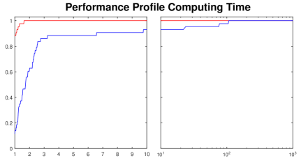
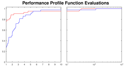
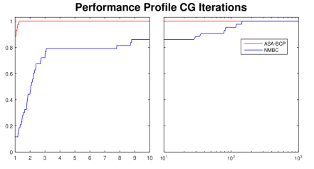
Figure 1: Comparison between ASA-BCP and NMBC: performance profiles on CPU time, number of objective function evaluations and number of conjugate gradient iterations. The $x$ axis is in linear scale in the left panel and in logarithmic scale in the right panel.

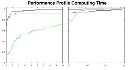
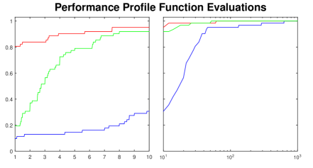
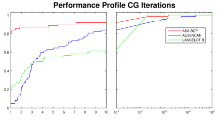
Figure 2: Comparison among ASA-BCP, ALGENCAN and LANCELOT B: performance profiles on CPU time, number of objective function evaluations and number of conjugate gradient iterations. The $x$ axis is in linear scale in the left panel and in logarithmic scale in the right panel.

These results seem to confirm that on the one hand, computing the search direction only in the subspace of the non-active variables guarantees some savings in terms of CPU time, and, on the other hand, getting rid of the Barzilai–Borwein step (used in NMBC) avoids the generation of badly scaled search directions.

In Figure 2, we show the performance profiles of ASA-BCP, ALGENCAN and LANCELOT B. By taking a look at the performance profiles related to CPU time, we can easily see that ASA-BCP and ALGENCAN are comparable in terms of efficiency and are both better than LANCELOT B. As regards robustness, we can see that ASA-BCP outperforms both ALGENCAN and LANCELOT B. More specifically, when $\tau$ is equal to $2$, ASA-BCP solves about $95\%$ of the problems, while ALGENCAN and LANCELOT B respectively, solve about $90\%$ and $30\%$ of the problems. Furthermore, ASA-BCP is able to solve all the problems when $\tau$ is about $70$, while ALGENCAN and LANCELOT B get to solve all the problems for significantly larger values of $\tau$.

For what concerns the number of objective function evaluations, ASA-BCP is the best in terms of efficiency and is competitive with LANCELOT B in terms of robustness. In particular, when $\tau$ is equal to $2$, ASA-BCP solves about $85\%$ of the problems, while ALGENCAN and LANCELOT B respectively, solve about $15\%$ and $30\%$ of the problems. Moreover, ASA-BCP and LANCELOT B solve all the problem when $\tau$ is about $60$ and $50$, respectively, while ALGENCAN gets to solve all the problems when $\tau$ is about $600$.

Finally, as regards the number of conjugate gradient iterations, ASA-BCP outperforms the other two codes in terms of efficiency, while LANCELOT B is the best in terms of robustness. More in detail, when $\tau$ is equal to $2$, ASA-BCP solves about $85\%$ of the problems, while ALGENCAN and LANCELOT B respectively, solve about $20\%$ and $35\%$ of the problems. LANCELOT B is able to solve all the problems when $\tau$ is about 200, while ASA-BCP and ALGENCAN need larger values of $\tau$.

6 Conclusions

In this paper, a two-stage active-set algorithm for box-constrained nonlinear programming problems is devised. In the first stage, we get a significant reduction in the objective function simply by setting to the bounds the estimated active variables. In the second stage, we employ a truncated-Newton direction computed in the subspace of the estimated non-active variables. These two stages are inserted in a non-monotone framework and the convergence of the resulting algorithm ASA-BCP is proved. Experimental results show that our implementation of ASA-BCP is competitive with other widely used codes for bound-constrained minimization problems.

Appendices

Appendix A

Proof of Proposition 2.

Assume that $\bar{x}$ satisfies (14)–(16). First, we show that

$$\bar{x}_{i}=l_{i},\quad\text{if }i\in A_{l}(\bar{x}),$$ (28)

$$\bar{x}_{i}=u_{i},\quad\text{if }i\in A_{u}(\bar{x}).$$ (29)

In order to prove (28), assume by contradiction that there exists an index $i\in A_{l}(\bar{x})$ such that $l_{i}<\bar{x}\leq l_{i}+\epsilon\lambda_{i}(\bar{x})$. It follows that $\lambda_{i}(\bar{x})>0$, and, from (12), that $g_{i}(\bar{x})>0$, contradicting (14). Then, (28) holds. The same reasoning applies to prove (29).
Recalling (9), we have that $g_{i}(\bar{x})>0$ for all $i\in A_{l}(\bar{x})$. Combined with (28), it means that $\bar{x}_{i}$ satisfies (2) for all $i\in A_{l}(\bar{x})$. Similarly, since $g_{i}(\bar{x})<0$ for all $i\in A_{u}(\bar{x})$ and (29) holds, then $\bar{x}_{i}$ satisfies (3) for all $i\in A_{u}(\bar{x})$.
From (16), we also have that $\bar{x}_{i}$ satisfies optimality conditions for all $i\in N(\bar{x})$. Then, $\bar{x}$ is a stationary point.
Now, assume that $\bar{x}$ is a stationary point. First, we consider a generic index $i$ such that $\bar{x}_{i}=l_{i}$. For such an index, from (2) we get $g_{i}(\bar{x})\geq 0$. If $g_{i}(\bar{x})>0$, then, from (9), it follows that $i\in A_{l}(\bar{x})$ and (14) is satisfied. Vice versa, if $g_{i}(\bar{x})=0$, then we have that $i$ belongs to $N(\bar{x})$, satisfying (16). The same reasoning applies for a generic index $i$ such that $\bar{x}_{i}=u_{i}$.
Finally, for every index $i$ such that $l_{i}<\bar{x}_{i}<u_{i}$, from (4) we have that $g_{i}(\bar{x})=0$. Then, $\bar{x}$ satisfies (14)–(16). ∎

Proof of Proposition 3.

Assume that (17) is verified. Namely,

$$\bar{x}_{i}=l_{i},\quad\text{if }i\in A_{l}(\bar{x}),$$

$$\bar{x}_{i}=u_{i},\quad\text{if }i\in A_{u}(\bar{x}).$$

Recalling the definition of $A_{l}(\bar{x})$ and $A_{u}(\bar{x})$, the previous relations imply that (14) and (15) are verified. Then, from Proposition 2, $\bar{x}$ is a stationary point if and only if $g_{i}(\bar{x})=0$ for all $i\in N(\bar{x})$. ∎

Proof of Proposition 4.

Assume that condition (18) is verified. If we have

$$\{i\in A_{l}(\bar{x})~{}\,~{}\colon\,\bar{x}_{i}>l_{i}\}~{}\cup~{}\{i\in A_{u}(\bar{x})~{}\,\colon\,\bar{x}_{i}<u_{i}\}=\emptyset,$$

from the definition of $A_{l}(\bar{x})$ and $A_{u}(\bar{x})$ it follows that

$$\bar{x}_{i}=l_{i}\,\text{ and }\,g_{i}(\bar{x})>0,\quad i\in A_{l}(\bar{x}),$$

$$\bar{x}_{i}=u_{i}\,\text{ and }\,g_{i}(\bar{x})<0,\quad i\in A_{u}(\bar{x}).$$

Then, conditions (2)–(4) are verified, and $\bar{x}$ is a stationary point.
Conversely, if $\bar{x}$ is a stationary point, we proceed by contradiction and assume that there exists $\bar{x}_{i}\in(l_{i},u_{i})$ such that $i\in A_{l}(\bar{x})\cup A_{u}(\bar{x})$. From the definition of $A_{l}(\bar{x})$ and $A_{u}(\bar{x})$, it follows that $g_{i}(\bar{x})\neq 0$, violating (4) and thus contradicting the fact that $\bar{x}$ is a stationary point.∎

Proof of Proposition 5.

By the second-order mean value theorem, we have

$$f(\tilde{x})=f(x)+g(x)^{T}(\tilde{x}-x)+\frac{1}{2}(\tilde{x}-x)^{T}H(z)(\tilde{x}-x),$$

where $z=x+\xi(\tilde{x}-x)$ for a $\xi\in]0,1[$. Therefore,

$$f(\tilde{x})-f(x)\leq g(x)^{T}(\tilde{x}-x)+\frac{1}{2}\bar{\lambda}\|x-\tilde{x}\|^{2}.\\$$ (30)

Recalling the definition of $\tilde{x}$, we can also write

$$g(x)^{T}(\tilde{x}-x)=\sum_{i\in A_{l}(x)}g_{i}(x)(l_{i}-x_{i})+\sum_{i\in A_{u}(x)}g_{i}(x)(u_{i}-x_{i}).$$ (31)

From the definitions of $A_{l}(x)$ and $A_{u}(x)$, and recalling (12) and (13), we have

$$g_{i}(x)\geq\frac{(x_{i}-l_{i})}{\epsilon}\left[\frac{(l_{i}-x_{i})^{2}+(u_{i}-x_{i})^{2}}{(u_{i}-x_{i})^{2}}\right],\quad i\in A_{l}(x),$$

$$g_{i}(x)\leq\frac{(x_{i}-u_{i})}{\epsilon}\left[\frac{(l_{i}-x_{i})^{2}+(u_{i}-x_{i})^{2}}{(l_{i}-x_{i})^{2}}\right],\quad i\in A_{u}(x),$$

and we can write

$$g_{i}(x)(l_{i}-x_{i})\leq-\frac{1}{\epsilon}(x_{i}-l_{i})^{2}\left[\frac{(l_{i}-x_{i})^{2}+(u_{i}-x_{i})^{2}}{(u_{i}-x_{i})^{2}}\right]\leq-\frac{1}{\epsilon}(l_{i}-x_{i})^{2},\quad i\in A_{l}(x),$$

$$g_{i}(x)(u_{i}-x_{i})\leq-\frac{1}{\epsilon}(u_{i}-x_{i})^{2}\left[\frac{(l_{i}-x_{i})^{2}+(u_{i}-x_{i})^{2}}{(u_{i}-x_{i})^{2}}\right]\leq-\frac{1}{\epsilon}(u_{i}-x_{i})^{2},\quad i\in A_{u}(x).$$

Hence, from (31), it follows that

$$g(x)^{T}(\tilde{x}-x)\leq-\frac{1}{\epsilon}\left[\sum_{i\in A_{l}(x)}(l_{i}-x_{i})^{2}+\sum_{i\in A_{u}(x)}(u_{i}-x_{i})^{2}\right]=-\frac{1}{\epsilon}\|x-\tilde{x}\|^{2}.$$ (32)

Finally, from (30) and (32), we have

$$f(\tilde{x})-f(x)\leq\frac{1}{2}\left(\bar{\lambda}-\frac{1}{\epsilon}\right)\|x-\tilde{x}\|^{2}-\frac{1}{2\epsilon}\|x-\tilde{x}\|^{2}\leq-\frac{1}{2\epsilon}\|x-\tilde{x}\|^{2},$$

where the last inequality follows from equation (19) in Assumption 1. ∎

Proof of Proposition 6.

Since the gradient is Lipschitz continuous over $[l,u]$, there exists $L<\infty$ such that for all $s\in[0,1]$ and for all $\alpha\geq 0$:

$$\|g(\bar{x})-g(\bar{x}-s[\bar{x}-\bar{x}(\alpha)])\|\leq sL\|\bar{x}-\bar{x}(\alpha)\|,\quad\forall\bar{x}\in[l,u].$$

By the mean value theorem, we have:

$$f(\bar{x}(\alpha))-f(\bar{x}) =g(\bar{x})^{T}(\bar{x}(\alpha)-x)+\int_{0}^{1}\big{(}g(\bar{x}-s[\bar{x}-\bar{x}(\alpha)])-g(\bar{x})\big{)}^{T}\big{(}\bar{x}(\alpha)-\bar{x}\big{)}\ ds$$

$$\leq g(\bar{x})^{T}(\bar{x}(\alpha)-\bar{x})+\|\bar{x}(\alpha)-\bar{x}\|\int_{0}^{1}sL\|\bar{x}(\alpha)-\bar{x}\|\ ds$$

$$=g(\bar{x})^{T}(\bar{x}(\alpha)-\bar{x})+\frac{L}{2}\|\bar{x}(\alpha)-\bar{x}\|^{2},\quad\forall\alpha\geq 0.$$ (33)

Moreover, as the gradient is continuous and the feasible set is compact, there exists $M>0$ such that

$$\|g(\bar{x})\|\leq M,\quad\forall\bar{x}\in[l,u].$$ (34)

From (20), (22) and (34), we can write

$$d_{i}\leq\|d\|\leq\sigma_{2}\|g(\bar{x})\|\leq\sigma_{2}M,\quad\forall\bar{x}\in[l,u],\quad\forall i=1,\dots,n.$$

Now, let us define $\theta_{1},\dots,\theta_{n}$ as:

$$\theta_{i}:=\begin{cases}\min\ \{\bar{x}_{i}-l_{i},u_{i}-\bar{x}_{i}\}\quad\text{ if }l_{i}<\bar{x}_{i}<u_{i},\\ u_{i}-l_{i}\qquad\qquad\qquad\quad\,\,\text{ otherwise},\end{cases}\qquad i=1,\dots,n.$$

We set

$$\tilde{\theta}:=\min_{i=1,\dots,n}\frac{\theta_{i}}{2},$$

and define $\hat{\alpha}$ as follows:

$$\hat{\alpha}:=\frac{\tilde{\theta}}{\sigma_{2}M}.$$

In the following, we want to majorize the right-hand-side term of (A). First, we consider the term $g(\bar{x})^{T}(\bar{x}(\alpha)-x)$. We distinguish three cases:

(i)

$i\in N(\bar{x})$ such that $l_{i}<\bar{x}_{i}<u_{i}$. We distinguish two subcases:

• if $d_{i}\geq 0$:

  $$l_{i}<\bar{x}_{i}+\alpha d_{i}\leq\bar{x}_{i}+\frac{\tilde{\theta}}{\sigma_{2}M}d_{i}\leq x_{i}+\tilde{\theta}<u_{i},\qquad\forall\alpha\in]0,\hat{\alpha}],$$

• else, if $d_{i}<0$:

  $$u_{i}>\bar{x}_{i}+\alpha d_{i}\geq\bar{x}_{i}+\frac{\tilde{\theta}}{\sigma_{2}M}d_{i}\geq\bar{x}_{i}-\tilde{\theta}>l_{i},\qquad\forall\alpha\in]0,\hat{\alpha}].$$

So, we have

$$\bar{x}_{i}(\alpha)=\bar{x}_{i}+\alpha d_{i},\quad\forall\alpha\in]0,\hat{\alpha}],$$

which implies

$$g_{i}(\bar{x})(\bar{x}_{i}(\alpha)-\bar{x}_{i})=\alpha g_{i}(\bar{x})d_{i},\quad\forall\alpha\in]0,\hat{\alpha}].$$ (35)

(ii)

$i\in N(\bar{x})$ such that $\bar{x}_{i}=l_{i}$. Recalling the definition of $N(x)$, it follows that $g_{i}(\bar{x})\leq 0$. We distinguish two subcases:

• if $d_{i}\geq 0$:

  $$l_{i}\leq\bar{x}_{i}+\alpha d_{i}\leq\bar{x}_{i}+\frac{\tilde{\theta}}{\sigma_{2}M}d_{i}\leq\bar{x}_{i}+\tilde{\theta}<u_{i},\qquad\forall\alpha\in]0,\hat{\alpha}],$$

  and then

  $$\bar{x}_{i}(\alpha)=\bar{x}_{i}+\alpha d_{i},\quad\forall\alpha\in]0,\hat{\alpha}],$$

  which implies

  $$g_{i}(\bar{x})(\bar{x}_{i}(\alpha)-\bar{x}_{i})=\alpha g_{i}(\bar{x})d_{i},\quad\forall\alpha\in]0,\hat{\alpha}].$$ (36)

• else, if $d_{i}<0$, we have

  $$\bar{x}_{i}(\alpha)=\bar{x}_{i},\quad\forall\alpha>0,$$

  and then

  $$0=g_{i}(\bar{x})(\bar{x}_{i}(\alpha)-\bar{x}_{i})\leq\alpha g_{i}(\bar{x})d_{i},\quad\forall\alpha>0.$$ (37)

(iii)

$i\in N(\bar{x})$ such that $\bar{x}_{i}=u_{i}$. Following the same reasonings done in the previous step, we have that

• if $d_{i}\leq 0$:

  $$g_{i}(\bar{x})(\bar{x}_{i}(\alpha)-\bar{x}_{i})=\alpha g_{i}(\bar{x})d_{i},\quad\forall\alpha\in]0,\hat{\alpha}];$$ (38)

• else, if $d_{i}>0$, we have

  $$0=g_{i}(\bar{x})(\bar{x}_{i}(\alpha)-\bar{x}_{i})\leq\alpha g_{i}(\bar{x})d_{i},\quad\forall\alpha>0.$$ (39)

From (20), (35), (36), (37), (38) and (39), we obtain

$$\begin{split}g(\bar{x})^{T}(\bar{x}(\alpha)-\bar{x})&=\sum_{i\in N(\bar{x})}g_{i}(\bar{x})(\bar{x}_{i}(\alpha)-\bar{x})\\ &\leq\alpha\sum_{i\in N(\bar{x})}g_{i}(\bar{x})d_{i}=\alpha g_{N(\bar{x})}(\bar{x})^{T}d_{N(\bar{x})},\quad\forall\alpha\in]0,\hat{\alpha}].\end{split}$$ (40)

Now, we consider the term $\displaystyle\frac{L}{2}\|\bar{x}(\alpha)-\bar{x}\|^{2}$. For every $i\in N(\bar{x})$ such that $d_{i}\leq 0$, we have that $0\leq\bar{x}_{i}-\bar{x}_{i}(\alpha)\leq-\alpha d_{i}$ holds for all $\alpha>0$. Therefore,

$$(\bar{x}_{i}-\bar{x}_{i}(\alpha))^{2}\leq\alpha^{2}d_{i}^{2},\quad\forall\alpha>0.$$ (41)

Else, for every $i\in N(\bar{x})$ such that $d_{i}>0$, we have that $0\leq\bar{x}_{i}(\alpha)-\bar{x}_{i}\leq\alpha d_{i}$ holds for all $\alpha>0$. Therefore,

$$0\leq(\bar{x}_{i}(\alpha)-\bar{x}_{i})^{2}\leq\alpha^{2}d_{i}^{2},\quad\forall\alpha>0.$$ (42)

Recalling (20), from (41) and (42) we obtain

$$\|\bar{x}(\alpha)-\bar{x}\|^{2}\leq\alpha^{2}\|d_{N(\bar{x})}\|^{2},\quad\forall\alpha>0.$$

Using (21) and (22), we get

$$\begin{split}\|\bar{x}(\alpha)-\bar{x}\|^{2}&\leq\alpha^{2}\|d_{N(\bar{x})}\|^{2}\leq\alpha^{2}\sigma_{2}^{2}\|g_{N(\bar{x})}(\bar{x})\|^{2}\\ &\leq-\alpha^{2}\frac{\sigma_{2}^{2}}{\sigma_{1}}g_{N(\bar{x})}(\bar{x})^{T}d_{N(\bar{x})},\quad\forall\alpha>0.\end{split}$$ (43)

From (20), (A), (40) and (43), we can write

$$\begin{split}f(\bar{x}(\alpha))-f(\bar{x})&\leq\alpha\left(1-\alpha\frac{L\sigma^{2}_{2}}{2\sigma_{1}}\right)g_{N(\bar{x})}(\bar{x})^{T}d_{N(\bar{x})}\\ &=\alpha\left(1-\alpha\frac{L\sigma^{2}_{2}}{2\sigma_{1}}\right)g(\bar{x})^{T}d,\quad\forall\alpha\in]0,\hat{\alpha}].\end{split}$$

It follows that (23) is satisfied by choosing $\bar{\alpha}$ such that

$$1-\bar{\alpha}\frac{L\sigma^{2}_{2}}{2\sigma_{1}}\geq\gamma,$$

$$\bar{\alpha}\in]0,\hat{\alpha}].$$

Thus, the proof is completed defining

$$\bar{\alpha}:=\min\left\{\hat{\alpha},\frac{2\sigma_{1}(1-\gamma)}{L\sigma^{2}_{2}}\right\}.$$

∎

Appendix B

The scheme of the algorithm is reported in Algorithm 1. At Step $10$, $17$ and $25$ there is the update of the reference value of the non-monotone line search $f^{j}_{R}$: we set $j:=j+1$, $l^{j}:=k$ and the reference value is updated according to the formula

$$f^{j}_{R}:=\max_{0\leq i\leq\min\{j,M\}}\bigl{\{}f^{j-i}\bigr{\}}.$$

Algorithm 1 ASA-BCP

$\,\,\,0$    Choose $x^{0}\in[l,u]$, fix $Z\geq 1$, $M\geq 0$, $\Delta_{0}\geq 0$, $\beta\in]0,1[$, $\delta\in]0,1[$, $\gamma\in]0,\frac{1}{2}[$, $k:=0$, $j:=-1$, $l^{-1}:=-1$, $f_{R}^{-1}:=f(x^{0})$, $f^{-1}:=f(x^{0})$, $\Delta=\tilde{\Delta}:=\Delta_{0}$, $checkpoint:=true$

$\,\,\,1$    While $x^{k}$ is a non-stationary point for problem (1)

$\,\,\,2$         Compute $A_{l}^{k}:=A_{l}(x^{k})$, $A_{u}^{k}:=A_{u}(x^{k})$ and $N^{k}:=N(x^{k})$

$\,\,\,3$         Set $\tilde{x}^{k}_{A_{l}^{k}}:=l_{A_{l}^{k}}$, $\tilde{x}^{k}_{A_{u}^{k}}:=u_{A_{u}^{k}}$ and $\tilde{x}^{k}_{N^{k}}:=x^{k}_{N^{k}}$

$\,\,\,4$         If $\|\tilde{x}^{k}-x^{k}\|\leq\tilde{\Delta}$, then set $\tilde{\Delta}=\beta\tilde{\Delta}$

$\,\,\,5$         Else compute $f(x^{k})$

$\,\,\,6$              If $f(x^{k})\geq f^{j}_{R}$, then backtrack to $\tilde{x}^{l^{j}}$, set $k:=l^{j}$ and go to Step $28$

$\,\,\,7$         End if

$\,\,\,8$         Compute $\tilde{A}_{l}^{k}:=A_{l}(\tilde{x}^{k})$, $\tilde{A}_{u}^{k}:=A_{u}(\tilde{x}^{k})$ and $\tilde{N}^{k}:=N(\tilde{x}^{k})$

$\,\,\,9$         If $\tilde{N}^{k}\neq\emptyset$ and $g_{\tilde{N}^{k}}(\tilde{x}^{k})\neq 0$

$10$              If $checkpoint=true$, then compute $f(\tilde{x}^{k})$ and update $f_{R}^{j}$

$11$                  Set $checkpoint:=false$

$12$              End if

$13$              Set $d^{k}_{\tilde{A}_{l}^{k}}:=0$, $d^{k}_{\tilde{A}_{u}^{k}}:=0$ and compute a gradient-related direction $d^{k}_{\tilde{N}^{k}}$ in $\tilde{x}^{k}$

$14$              If $k\geq l^{j}+Z$, then compute $f(\tilde{x}^{k})$

$15$                  If $f(\tilde{x}^{k})\geq f^{j}_{R}$

$16$                       Backtrack to $\tilde{x}^{l^{j}}$, set $d^{k}:=d^{l^{j}}$, $k:=l^{j}$ and go to Step $28$

$17$                  Else update $f_{R}^{j}$

$18$                  End if

$19$              End if

$20$              If $\|{d^{k}_{\tilde{N}^{k}}}\|\leq\Delta$

$21$                  Set $\alpha^{k}:=1$, $x^{k+1}:=[\tilde{x}^{k}+\alpha^{k}d^{k}]^{\sharp}$, $\Delta:=\beta\Delta$, $k:=k+1$

$22$              Else if $k\neq l^{j}$, then compute $f(\tilde{x}^{k})$

$23$                  If $f(\tilde{x}^{k})\geq f^{j}_{R}$

$24$                       Backtrack to $\tilde{x}^{l^{j}}$, set $d^{k}:=d^{l^{j}}$, $k:=l^{j}$ and go to Step $28$

$25$                  Else update $f_{R}^{j}$

$26$                  End if

$27$              End if

$28$              Set $\alpha^{k}:=\delta^{\nu}$, where $\nu$ is the smallest nonnegative integer for which

$$f([\tilde{x}^{k}+\delta^{\nu}d^{k}]^{\sharp})\leq f^{j}_{R}+\gamma\delta^{\nu}g(\tilde{x}^{k})^{T}d^{k}$$

$29$              Set $x^{k+1}:=[\tilde{x}^{k}+\alpha^{k}d^{k}]^{\sharp}$, $k:=k+1$, $checkpoint:=true$

$30$         Else

$31$              Set $\alpha^{k}:=0$, $d^{k}:=0$, $x^{k+1}:=[\tilde{x}^{k}+\alpha^{k}d^{k}]^{\sharp}$, $k:=k+1$

$32$         End if

$33$    End while

Appendix C

In this section, we prove Theorem 1. Preliminarily, we need to state some results.

Lemma 1.

Let Assumption 1 hold. Suppose that ASA-BCP produces an infinite sequence $\{x^{k}\}$, then

1. $\{f^{j}_{R}\}$ is non-increasing and converges to a value $\bar{f}_{R}$;

2. for any fixed $j\geq 0$ we have:

   $$f^{h}_{R}<f^{j}_{R},\quad\forall h>j+M.$$

Proof.

The proof follows from Lemma 1 in [23]. ∎

Lemma 2.

Let Assumption 1 hold. Suppose that ASA-BCP produces an infinite sequence $\{x^{k}\}$ and an infinite sequence $\{\tilde{x}^{k}\}$. For any given value of $k$, let $q(k)$ be the index such that

$$q(k):=\max\{j\colon l^{j}\leq k\}.$$

Then, there exists a sequence $\{\tilde{x}^{s(j)}\}$ and an integer $L$ satisfying the following conditions:

1. $f^{j}_{R}=f(\tilde{x}^{s(j)})$

2. for any integer $k$, there exist an index $h^{k}$ and an index $j^{k}$ such that:

   $$0<h^{k}-k\leq L,\qquad h^{k}=s(j^{k}),$$

   $$f^{j^{k}}_{R}=f(\tilde{x}^{h^{k}})<f^{q(k)}_{R}.$$

Proof.

The proof follows from Lemma $2$ in [23] taking into account that for any iteration index $k$, there exists an integer $\tilde{L}$ such that the condition of Step $9$ is satisfied within the $(k+\tilde{L})$-th iteration. In fact, assume by contradiction that it is not true. If Step $9$ is not satisfied at a generic iteration $k$, then $x^{k+1}=\tilde{x}^{k}$. Since the sequences $\{x^{k}\}$ and $\{\tilde{x}^{k}\}$ are infinite, Proposition 4 implies that $\tilde{x}^{k+1}\neq x^{k+1}$ and that the objective function strictly decreases. Repeating this procedure for an infinite number of steps, an infinite sequence of distinct points $\{x^{k+1},x^{k+2},\dots\}$ is produced, where these points differ from each other only for the values of the variables at the bounds. Since the number of variables is finite, this produces a contradiction. ∎

Lemma 3.

Let Assumption 1 hold. Suppose that ASA-BCP produces an infinite sequence $\{x^{k}\}$ and an infinite sequence $\{\tilde{x}^{k}\}$. Then,

$$\lim_{k\to\infty}f(x^{k})=\lim_{k\to\infty}f(\tilde{x}^{k})=\lim_{j\rightarrow\infty}f^{j}_{R}=\bar{f}_{R},$$ (44)

$$\lim_{k\to\infty}\|x^{k+1}-\tilde{x}^{k}\|=\lim_{k\to\infty}\alpha^{k}\|d^{k}\|=0,$$ (45)

$$\lim_{k\to\infty}\|\tilde{x}^{k}-x^{k}\|=0.$$ (46)

Proof.

We build two different partitions of the iterations indices to analyze the computation of $x^{k+1}$ from $\tilde{x}^{k}$ and that of $\tilde{x}^{k}$ from $x^{k}$, respectively. From the instructions of the algorithm, it follows that $x^{k+1}$ can be computed at Step $21$, Step $29$ or Step $31$. Let us consider the following subset of iteration indices:

$$\mathcal{K}_{1}:=\{k\colon x^{k+1}\text{ is computed at Step $21$}\},$$

$$\mathcal{K}_{2}:=\{k\colon x^{k+1}\text{ is computed at Step $29$}\},$$

$$\mathcal{K}_{3}:=\{k\colon x^{k+1}\text{ is computed at Step $31$}\}.$$

Then, we have

$$\mathcal{K}_{1}\cup\mathcal{K}_{2}\cup\mathcal{K}_{3}=\{0,1,\dots\}.$$

As regards the computation of $\tilde{x}^{k}$, we distinguish two further subsets of iterations indices:

$$\mathcal{K}_{4}:=\{k\colon\tilde{x}^{k}\text{ satisfies the test at Step $4$}\},$$

$$\mathcal{K}_{5}:=\{k\colon\tilde{x}^{k}\text{ does not satisfy the test at Step $4$}\}.$$

Then, we have

$$\mathcal{K}_{4}\cup\mathcal{K}_{5}=\{0,1,\dots\}.$$

Preliminarily, we point out some properties of the above subsequences. The subsequence $\{\tilde{x}^{k}\}_{\mathcal{K}_{1}}$ satisfies

$$\|x^{k+1}-\tilde{x}^{k}\|=\alpha^{k}\|d^{k}\|=\|d^{k}\|\leq\beta^{t}\Delta_{0},\quad k\in\mathcal{K}_{1},$$

where the integer $t$ increases with $k\in\mathcal{K}_{1}$. Since $\beta\in]0,1)$, if $\mathcal{K}_{1}$ is infinite, we have

$$\lim_{k\to\infty,\,k\in\mathcal{K}_{1}}\|x^{k+1}-\tilde{x}^{k}\|=\lim_{k\to\infty,\,k\in\mathcal{K}_{1}}\alpha^{k}\|d^{k}\|=0.$$ (47)

Moreover, since $\alpha^{k}=0$ and $d^{k}=0$ for all $k\in\mathcal{K}_{3}$, if $\mathcal{K}_{3}$ is infinite, we have

$$\lim_{k\to\infty,\,k\in\mathcal{K}_{3}}\|x^{k+1}-\tilde{x}^{k}\|=\lim_{k\to\infty,\,k\in\mathcal{K}_{3}}\alpha^{k}\|d^{k}\|=0.$$ (48)

The subsequence $\{\tilde{x}^{k}\}_{\mathcal{K}_{4}}$ satisfies

$$\|\tilde{x}^{k}-x^{k}\|\leq\beta^{t}\tilde{\Delta}_{0},\quad k\in\mathcal{K}_{4},$$

where the integer $t$ increases with $k\in\mathcal{K}_{4}$. Since $\beta\in]0,1[$, if $\mathcal{K}_{4}$ is infinite, we have

$$\lim_{k\to\infty,\,k\in\mathcal{K}_{4}}\|\tilde{x}^{k}-x^{k}\|=0.$$ (49)

Now we prove (44). Let $s(j)$, $h^{k}$ and $q(k)$ be the indices defined in Lemma 2. We show that for any fixed integer $i\geq 1$, the following relations hold:

$$\lim_{j\to\infty}\|\tilde{x}^{s(j)-i+1}-x^{s(j)-i+1}\|=0,$$ (50)

$$\lim_{j\to\infty}\|x^{s(j)-i+1}-\tilde{x}^{s(j)-i}\|=\lim_{j\to\infty}\alpha^{s(j)-i}\|d^{s(j)-i}\|=0,$$ (51)

$$\lim_{j\to\infty}f(x^{s(j)-i+1})=\bar{f}_{R},$$ (52)

$$\lim_{j\to\infty}f(\tilde{x}^{s(j)-i})=\bar{f}_{R}.$$ (53)

Without loss of generality, we assume that $j$ is large enough to avoid the occurrence of negative apices. We proceed by induction and first show that (50)–(53) hold for $i=1$. If $s(j)\in\mathcal{K}_{4}$, relations (50) and (52) follow from (49) and the continuity of the objective function. If $s(j)\in\mathcal{K}_{5}$, from the instructions of the algorithm and taking into account Proposition 5, we get

$$f^{j}_{R}=f(\tilde{x}^{s(j)})\leq f(x^{s(j)})-\dfrac{1}{2\epsilon}\|x^{s(j)}-\tilde{x}^{s(j)}\|^{2}<f^{j-1}_{R},$$

from which we get

$$f^{j}_{R}=f(\tilde{x}^{s(j)})\leq f(x^{s(j)})<f^{j-1}_{R},$$

and then, from point (i) of Lemma 1, it follows that

$$\lim_{j\to\infty}f(\tilde{x}^{s(j)})=\lim_{j\to\infty}f(x^{s(j)})=\bar{f}_{R},$$ (54)

which proves (52) for $i=1$. From the above relation, and by exploiting Proposition 5 again, we have that

$$\lim_{j\to\infty}\bigl{(}f(\tilde{x}^{s(j)})-f(x^{s(j)})\bigr{)}\leq\lim_{j\to\infty}-\dfrac{1}{2\epsilon}\|x^{s(j)}-\tilde{x}^{s(j)}\|^{2}.$$

and then (50) holds for $i=1$.
If $s(j)-1\in\mathcal{K}_{1}\cup\mathcal{K}_{3}$, from (47) and (48) it is straightforward to verify that (51) holds for $i=1$. By exploiting the continuity of the objective function, since (51) and (52) hold for $i=1$, then also (53) is verified for $i=1$. If $s(j)-1\in\mathcal{K}_{2}$, from the instruction of the algorithm, we obtain

$$f(x^{s(j)})=f(\tilde{x}^{s(j)-1}+\alpha^{s(j)-1}d^{s(j)-1})\leq f^{q(s(j)-1)}_{R}+\gamma\alpha^{s(j)-1}g(\tilde{x}^{s(j)-1})^{T}d^{s(j)-1},$$

and then

$$f(x^{s(j)})-f^{q(s(j)-1)}_{R}\leq\gamma\alpha^{s(j)-1}g(\tilde{x}^{s(j)-1})^{T}d^{s(j)-1}.$$

From (54), point (i) of Lemma 1, and recalling (20)–(22), we have that

$$\lim_{j\to\infty}\alpha^{s(j)-1}\|d^{s(j)-1}\|=\lim_{j\to\infty}\|x^{s(j)}-\tilde{x}^{s(j)-1}\|=0$$

for every subsequence such that $s(j)-1\in\mathcal{K}_{2}$. Therefore, (51) holds for $i=1$. Recalling that $f(x^{s(j)})=f(\tilde{x}^{s(j)-1}+\alpha^{s(j)-1}d^{s(j)-1})$, and since (50) and (51) hold for $i=1$, from the continuity of the objective function it follows that also (53) holds for $i=1$.
Now we assume that (50)–(53) hold for a given fixed $i\geq 1$ and show that these relations must hold for $i+1$ as well. If $s(j)-i\in\mathcal{K}_{4}$, by using (49), it is straightforward to verify that (50) is verified replacing $i$ with $i+1$. Taking into account (53), this implies that

$$\lim_{j\to\infty}f(x^{s(j)-(i+1)+1})=\lim_{j\to\infty}f(x^{s(j)-i})=\lim_{j\to\infty}f(\tilde{x}^{s(j)-i})=\bar{f}_{R},$$

and then (52) holds for $i+1$. If $s(j)-i\in\mathcal{K}_{5}$, from the instructions of the algorithm, and taking into account Proposition 5, we get

$$f(\tilde{x}^{s(j)-i})\leq f(x^{s(j)-i})-\dfrac{1}{2\epsilon}\|x^{s(j)-i}-\tilde{x}^{s(j)-i}\|^{2}<f^{q(s(j)-i)-1}_{R}.$$

Exploiting (53) and point (i) of Lemma 1, we have that

$$\lim_{j\to\infty}f(\tilde{x}^{s(j)-i})=\lim_{j\to\infty}f(x^{s(j)-i})=\bar{f}_{R},$$ (55)

which proves (52) for $i+1$. From the above relation, and by exploiting Proposition 5 again, we can also write

$$\lim_{j\to\infty}\bigl{(}f(\tilde{x}^{s(j)-i})-f(x^{s(j)}-i)\bigr{)}\leq\lim_{j\to\infty}-\dfrac{1}{2\epsilon}\|x^{s(j)-i}-\tilde{x}^{s(j)-i}\|^{2}.$$

and then (50) holds for $i+1$.
If $s(j)-i-1\in\mathcal{K}_{1}\cup\mathcal{K}_{3}$, from (47) and (48), we obtain that (51) holds for $i=i+1$. Since $x^{s(j)-i}=\tilde{x}^{s(j)-i-1}+\alpha^{s(j)-i-1}d^{s(j)-i-1}$, exploiting (47), (48), (55) and the continuity of the objective function, we obtain that (53) holds replacing $i$ with $i+1$.
If $s(j)-i-1\in\mathcal{K}_{2}$, from the instruction of the algorithm, we obtain

$$\begin{split}f(x^{s(j)-i})&=f(\tilde{x}^{s(j)-i-1}+\alpha^{s(j)-i-1}d^{s(j)-i-1})\\ &\leq f^{q(s(j)-i-1)}_{R}+\gamma\alpha^{s(j)-i-1}g(\tilde{x}^{s(j)-i-1})^{T}d^{s(j)-i-1},\end{split}$$

and then

$$f(x^{s(j)-i})-f^{q(s(j)-i-1)}_{R}\leq\gamma\alpha^{s(j)-i-1}g(\tilde{x}^{s(j)-i-1})^{T}d^{s(j)-i-1}.$$

From (55), point (i) of Lemma 1, and recalling (20)–(22), we have that

$$\lim_{j\to\infty}\alpha^{s(j)-i-1}\|d^{s(j)-i-1}\|=\lim_{j\to\infty}\|x^{s(j)-i}-\tilde{x}^{s(j)-i-1}\|=0$$

for every subsequence such that $s(j)-1\in\mathcal{K}_{2}$. Therefore, (51) holds for $i+1$.
Recalling that $f(x^{s(j)-i})=f(\tilde{x}^{s(j)-i-1}+\alpha^{s(j)-i-1}d^{s(j)-i-1})$, and since (50) and (51) hold replacing $i$ with $i+1$, exploiting the continuity of the objective function, we have

$$\lim_{j\to\infty}f(\tilde{x}^{s(j)-i-1}+\alpha^{s(j)-i-1}d^{s(j)-i-1})=\lim_{j\to\infty}f(x^{s(j)-i})=\lim_{j\to\infty}f(\tilde{x}^{s(j)-i}).$$

Therefore, if (53) holds at a generic $i\geq 1$, it must hold for $i+1$ as well. This completes the induction.
Now, for any iteration index $k>0$, we can write

$$\begin{split}&\tilde{x}^{h^{k}}=x^{k}+\sum_{i=0}^{h^{k}-k}\bigl{(}\tilde{x}^{h^{k}-i}-x^{h^{k}-i}\bigr{)}+\sum_{i=1}^{h^{k}-k}\alpha^{h^{k}-i}d^{h^{k}-i},\\ &\tilde{x}^{h^{k}}=\tilde{x}^{k}+\sum_{i=0}^{h^{k}-k-1}\bigl{(}\tilde{x}^{h^{k}-i}-x^{h^{k}-i}\bigr{)}+\sum_{i=1}^{h^{k}-k}\alpha^{h^{k}-i}d^{h^{k}-i}.\end{split}$$

From (50) and (51), we obtain

$$\lim_{k\to\infty}\|x^{k}-\tilde{x}^{h^{k}}\|=\lim_{k\to\infty}\|\tilde{x}^{k}-\tilde{x}^{h^{k}}\|=0.$$

By exploiting the continuity of the objective function, and taking into account point (i) of Lemma 1, the above relation implies that

$$\lim_{k\to\infty}f(x^{k})=\lim_{k\to\infty}f(\tilde{x}^{k})=\lim_{k\to\infty}f(\tilde{x}^{h^{k}})=\lim_{k\to\infty}f^{j}_{R}=\bar{f}_{R},$$

which proves (44).
To prove (45), if $k\in\mathcal{K}_{1}\cup\mathcal{K}_{3}$, then from (47) and (48) we obtain

$$\lim_{k\to\infty,\,k\in\mathcal{K}_{1}\cup\mathcal{K}_{3}}\|x^{k+1}-\tilde{x}^{k}\|=\lim_{k\to\infty,\,k\in\mathcal{K}_{1}\cup\mathcal{K}_{3}}\alpha^{k}\|d^{k}\|=0.$$ (56)

If $k\in\mathcal{K}_{2}$, from the instruction of the algorithm, we get

$$f(x^{k+1})\leq f(\tilde{x}^{q(k)})+\gamma\alpha^{k}g(\tilde{x}^{k})^{T}d^{k},$$

and then, recalling conditions (20)–(22) and (44), we can write

$$\lim_{k\to\infty,\,k\in\mathcal{K}_{2}}\|x^{k+1}-\tilde{x}^{k}\|=\lim_{k\to\infty,\,k\in\mathcal{K}_{2}}\alpha^{k}\|d^{k}\|=0.$$ (57)

From (56) and (57), it follows that (45) holds.
To prove (46), if $k\in\mathcal{K}_{4}$, then from (49) we obtain

$$\lim_{k\to\infty,\,k\in\mathcal{K}_{4}}\|\tilde{x}^{k}-x^{k}\|=0.$$ (58)

If $k\in\mathcal{K}_{5}$, from the instruction of the algorithm and recalling Proposition 5, we get

$$f(\tilde{x}^{k})\leq f(x^{k})-\dfrac{1}{2\epsilon}\|x^{k}-\tilde{x}^{k}\|^{2}<f^{q(k)-1}_{R}.$$

From (44) and point (i) of Lemma 1, we have that

$$\lim_{k\to\infty,\,k\in\mathcal{K}_{5}}f(\tilde{x}^{k})=\lim_{k\to\infty,\,k\in\mathcal{K}_{5}}f(x^{k})=\bar{f}_{R}.$$

By exploiting Proposition 5 again, we can write

$$\lim_{k\to\infty,\,k\in\mathcal{K}_{5}}\bigl{(}f(\tilde{x}^{k})-f(x^{k})\bigr{)}\leq\lim_{k\to\infty,\,k\in\mathcal{K}_{5}}-\dfrac{1}{2\epsilon}\|x^{k}-\tilde{x}^{k}\|^{2}=0,$$

and then

$$\lim_{k\to\infty,\,k\in\mathcal{K}_{5}}\|\tilde{x}^{k}-x^{k}\|=0.$$ (59)

From (58) and (59), it follows that (46) holds.∎

The following theorem extends a known result from unconstrained optimization, guaranteeing that the sequence of the directional derivatives along the search direction converges to zero.

Theorem 3.

Let Assumption 1 hold. Assume that ASA-BCP does not terminate in a finite number of iterations, and let $\{x^{k}\}$, $\{\tilde{x}^{k}\}$ and $\{d^{k}\}$ be the sequences produced by the algorithm. Then,

$$\lim_{k\to\infty}g(\tilde{x}^{k})^{T}d^{k}=0.$$ (60)

Proof.

We can identify two iteration index subsets $H,K\subseteq\{1,2,\dots\}$, such that:

• $N(\tilde{x}^{k})\neq\emptyset$ and $g_{N}(\tilde{x}^{k})\neq 0$, for all $k\in K$,

• $H:=\{1,2,\dots\}\setminus K$.

By assumption, the algorithm does not terminate in a finite number of iterations, and then, at least one of the above sets is infinite. Since we are interested in the asymptotic behavior of the sequence produced by ASA-BCP, we assume without loss of generality that both $H$ and $K$ are infinite sets.
Taking into account Step $31$ in Algorithm 1, it is straightforward to verify that

$$\lim_{k\to\infty,\,k\in H}g(\tilde{x}^{k})^{T}d^{k}=0.$$

Therefore, we limit our analysis to consider the subsequence $\{x^{k}\}_{K}$. Let $\bar{x}$ be any limit point of $\{x^{k}\}_{K}$. By contradiction, we assume that (60) does not hold. Using (46) of Lemma 3, since $\{x^{k}\}$, $\{\tilde{x}^{k}\}$ and $\{d^{k}\}$ are limited, and taking into account that $A_{l}(x^{k})$, $A_{u}(x^{k})$ and $N(x^{k})$ are subsets of a finite set of indices, without loss of generality we redefine $\{x^{k}\}_{K}$ the subsequence such that

$$\lim_{k\to\infty,\,k\in K}x^{k}=\lim_{k\to\infty,\,k\in K}\tilde{x}^{k}=\bar{x},$$

and

$$N^{k}:=\hat{N},\quad A_{l}^{k}:=\hat{A}_{l},\quad A_{u}^{k}:=\hat{A}_{u},\quad\forall k\in K,$$

$$\lim_{k\to\infty,\,k\in K}d^{k}=\hat{d}.$$

Since we have assumed that (60) does not hold, the above relations, combined with (21) and the continuity of the gradient, imply that

$$\lim_{k\to\infty,\,k\in K}g(\tilde{x}^{k})^{T}d^{k}=g(\bar{x})^{T}\hat{d}=-\eta<0.$$ (61)

It follows that

$$\lim_{k\to\infty,\,k\in K}\hat{d}\neq 0,$$

and then, recalling (45) of Lemma 3, we get

$$\lim_{k\to\infty,\,k\in K}\alpha^{k}=0.$$ (62)

Consequently, from the instructions of the algorithm, there must exist a subsequence (renamed $K$ again) such that the line search procedure at Step $28$ is performed and $\alpha^{k}<1$ for sufficiently large $k$. Namely,

$$\begin{split}f\bigl{(}\bigl{[}\tilde{x}^{k}+\frac{\alpha^{k}}{\delta}d^{k}\bigr{]}^{\sharp}\bigr{)}&>f^{q(k)}_{R}+\gamma\frac{\alpha^{k}}{\delta}g(\tilde{x}^{k})^{T}d^{k}\\ &\geq f(\tilde{x}^{k})+\gamma\frac{\alpha^{k}}{\delta}g(\tilde{x}^{k})^{T}d^{k},\quad\forall k\geq\bar{k},\,k\in K,\end{split}$$ (63)

where $q(k):=\max\{j\colon l^{j}\leq k\}$. We can write the point $[\tilde{x}^{k}+\frac{\alpha^{k}}{\delta}d^{k}]^{\sharp}$ as follows:

$$\bigl{[}\tilde{x}^{k}+\frac{\alpha^{k}}{\delta}d^{k}\bigl{]}^{\sharp}=\tilde{x}^{k}+\frac{\alpha^{k}}{\delta}d^{k}-y^{k},$$ (64)

where

$$y^{k}_{i}:=\max\bigl{\{}0,\bigl{(}\tilde{x}^{k}+\frac{\alpha^{k}}{\delta}d^{k}\bigr{)}_{i}-u_{i}\bigr{\}}-\max\bigl{\{}0,l_{i}-\bigl{(}\tilde{x}^{k}+\frac{\alpha^{k}}{\delta}d^{k}\bigr{)}_{i}\bigr{\}},\quad i=1,\dots,n.$$

As $\{\tilde{x}^{k}\}$ is a sequence of feasible points, $\{\alpha^{k}\}$ converges to zero and $\{d^{k}\}$ is limited, we get

$$\lim_{k\to\infty,\,k\in K}y^{k}=0.$$ (65)

From (63) and (64), we can write

$$f\bigl{(}\tilde{x}^{k}+\frac{\alpha^{k}}{\delta}d^{k}-y^{k}\bigr{)}-f(\tilde{x}^{k})>\gamma\frac{\alpha^{k}}{\delta}g(\tilde{x}^{k})^{T}d^{k},\quad\forall k\geq\bar{k},\,k\in K.$$ (66)

By the mean value theorem, we have

$$f\bigl{(}\tilde{x}^{k}+\frac{\alpha^{k}}{\delta}d^{k}-y^{k}\bigr{)}=f(\tilde{x}^{k})+\frac{\alpha^{k}}{\delta}g(z^{k})^{T}d^{k}-g(z^{k})^{T}y^{k},$$ (67)

where

$$z^{k}=\tilde{x}^{k}+\theta^{k}\bigl{(}\frac{\alpha^{k}}{\delta}d^{k}-y^{k}\bigr{)},\quad\theta^{k}\in]0,1[.$$ (68)

From (62) and (65), and since $\{d^{k}\}$ is limited, we obtain

$$\lim_{k\to\infty,\,k\in K}z^{k}=\bar{x}.$$ (69)

Substituting (67) into (66), and multiplying each term by $\dfrac{\delta}{\alpha^{k}}$, we get

$$g(z^{k})^{T}d^{k}-\frac{\delta}{\alpha^{k}}g(z^{k})^{T}y^{k}>\gamma g(\tilde{x}^{k})^{T}d^{k},\quad\forall k\geq\bar{k},\,k\in K.$$ (70)

From the definition of $y^{k}$, it follows that

$$y^{k}_{i}=\begin{cases}0,\qquad&\text{ if }l_{i}\leq\tilde{x}^{k}_{i}+\frac{\alpha^{k}}{\delta}d^{k}_{i}\leq u_{i},\\ \tilde{x}^{k}_{i}+\frac{\alpha^{k}}{\delta}d^{k}_{i}-u_{i}>0,\qquad&\text{ if }\tilde{x}^{k}_{i}+\frac{\alpha^{k}}{\delta}d^{k}_{i}>u_{i},\\ \tilde{x}^{k}_{i}+\frac{\alpha^{k}}{\delta}d^{k}_{i}-l_{i}<0,\qquad&\text{ if }l_{i}>\tilde{x}^{k}_{i}+\frac{\alpha^{k}}{\delta}d^{k}_{i}.\end{cases}$$ (71)

In particular, we have

$$y^{k}_{i}\begin{cases}=0,\quad&\text{ if }d^{k}_{i}=0,\\ \in[0,\frac{\alpha^{k}}{\delta}d^{k}_{i}],\quad&\text{ if }d^{k}_{i}>0,\\ \in[-\frac{\alpha^{k}}{\delta}d^{k}_{i},0],\quad&\text{ if }d^{k}_{i}<0.\end{cases}$$ (72)

From the above relation, it is straightforward to verify that

$$|y^{k}_{i}|\leq\frac{\alpha^{k}}{\delta}|d^{k}_{i}|,\quad i=1,\dots,n.$$ (73)

In the following, we want to majorize the left-hand side of (70) by showing that $\{\frac{\alpha^{k}}{\delta}g(z^{k})^{T}y^{k}\}$ converges to a nonnegative value. To this aim, we analyze three different cases, depending on whether $\bar{x}_{i}$ is at the bounds or is strictly feasible:

(i)

$i\in\hat{N}$ such that $l_{i}<\bar{x}_{i}<u_{i}$. As $\{\tilde{x}^{k}\}$ converges to $\bar{x}$, there exists $\tau>0$ such that

$$l_{i}+\tau\leq\tilde{x}^{k}\leq u_{i}-\tau,\qquad k\in K,\,k\text{ sufficiently large}.$$

Since $\{\alpha^{k}\}$ converges to zero and $\{d^{k}\}$ is limited, it follows that $\frac{\alpha^{k}}{\delta}|d^{k}_{i}|<\tau$, for $k\in K$, $k$ sufficiently large. Then,

$$l_{i}<\tilde{x}^{k}_{i}+\frac{\alpha^{k}}{\delta}d^{k}_{i}<u_{i},\qquad k\in K,\,k\text{ sufficiently large},$$

which implies, from (71), that

$$y^{k}_{i}=0,\qquad k\in K,\,k\text{ sufficiently large}.$$ (74)

(ii)

$i\in\hat{N}$ such that $\bar{x}_{i}=l_{i}$. First, we show that

$$g_{i}(\bar{x})\leq 0,$$ (75)

$$y^{k}_{i}\leq 0,\qquad k\in K,\,k\text{ sufficiently large}.$$ (76)

To show (75), we assume by contradiction that $g_{i}(\bar{x})>0$. From (12) and recalling that $\|\tilde{x}^{k}-x^{k}\|$ converges to zero from (46) of Lemma 3, it follows that

$$\lim_{k\to\infty,\,k\in K}\lambda_{i}(\tilde{x}^{k})=\lim_{k\to\infty,\,k\in K}g_{i}(\tilde{x}^{k})=g_{i}(\bar{x})>0.$$

Then, there exist an iteration index $\hat{k}$ and a scalar $\xi>0$ such that $\lambda_{i}(\tilde{x}^{k})\geq\xi>0$, for all $k\geq\hat{k},\,k\in K$. As $\{\tilde{x}^{k}_{i}\}$ converges to $l_{i}$, there also exists $\tilde{k}\geq\hat{k}$ such that

$$l_{i}\leq\tilde{x}^{k}_{i}\leq l_{i}+\epsilon\xi\leq l_{i}+\epsilon\lambda_{i}(\tilde{x}^{k}), \qquad k\in K,\,k\geq\tilde{k},$$

$$g_{i}(\tilde{x}^{k})>0, \qquad k\in K,\,k\geq\tilde{k},$$

which contradicts the fact that $i\in N(\tilde{x}^{k})$ for $k$ sufficiently large. To show (76), we observe that since $\{\tilde{x}^{k}_{i}\}$ converges to $l_{i}$, there exists $\tau\in]0,u_{i}-l_{i}]$ such that

$$l_{i}\leq\tilde{x}^{k}_{i}\leq u_{i}-\tau,\qquad k\in K,\,k\text{ sufficiently large}.$$

Moreover, since $\{\alpha^{k}\}$ converges to zero and $\{d^{k}\}$ is limited, it follows that $\frac{\alpha^{k}}{\delta}d^{k}_{i}\leq\tau$, for $k\in K$, $k$ sufficiently large. Then,

$$\tilde{x}^{k}+\frac{\alpha^{k}}{\delta}d^{k}_{i}\leq u_{i},\qquad k\in K,\,k\text{ sufficiently large}.$$

The above relation, combined with (71), proves (76). Now, we distinguish two subcases, depending on the sign of $d^{k}_{i}$:

• for every subsequence $\bar{K}\subseteq K$ such that $d^{k}_{i}\geq 0$, from (72) it follows that $y^{k}_{i}\geq 0$. Consequently, from (76) we can write

  $$y^{k}_{i}=0,\qquad k\in\bar{K},\,k\text{ sufficiently large}.$$ (77)

• for every subsequence $\bar{K}\subseteq K$ such that $d^{k}_{i}<0$, we have two further possible situations, according to (75):

  • $g_{i}(\bar{x})<0$. As $\{z^{k}\}$ converges to $\bar{x}$, then $g_{i}(z^{k})\leq 0$ for $k\in\bar{K}$, $k$ sufficiently large. From (76), we obtain

    $$\frac{\delta}{\alpha^{k}}g_{i}(z^{k})y^{k}_{i}\geq 0,\qquad k\in\bar{K},\,k\text{ sufficiently large}.$$ (78)

  • $g_{i}(\bar{x})=0$. From (73), we get

    $$\frac{\delta}{\alpha^{k}}|g_{i}(z^{k})y^{k}_{i}|\leq\frac{\delta}{\alpha^{k}}|g_{i}(z^{k})||y^{k}_{i}|\leq|g_{i}(z^{k})||d^{k}_{i}|.$$

    Since $\{d^{k}\}$ is limited, $\{z^{k}\}$ converges to $\bar{x}$, and $g_{i}(\bar{x})=0$, from the continuity of the gradient we get

    $$\lim_{k\to\infty,\,k\in\bar{K}}\frac{\delta}{\alpha^{k}}g_{i}(z^{k})d^{k}_{i}=0.$$ (79)

(iii)

$i\in\hat{N}$ such that $\bar{x}_{i}=u_{i}$. Reasoning as in the previous case, we obtain

$$\lim_{k\to\infty,\,k\in K}\frac{\delta}{\alpha^{k}}g_{i}(z^{k})y^{k}_{i}\geq 0.$$ (80)

Finally, from (74), (77), (78), (79) and (80), we have

$$\lim_{k\to\infty,\,k\in K}\frac{\delta}{\alpha^{k}}g(z^{k})^{T}y^{k}\geq 0,$$ (81)

and, from (61), (69), (70), (80) and (81), we obtain

$$\begin{split}-\eta&=\lim_{\begin{subarray}{c}k\to\infty\\ k\in K\end{subarray}}g(\tilde{x}^{k})^{T}d^{k}=\lim_{\begin{subarray}{c}k\to\infty\\ k\in K\end{subarray}}g(z^{k})^{T}d^{k}\geq\lim_{\begin{subarray}{c}k\to\infty\\ k\in K\end{subarray}}g(z^{k})^{T}d^{k}-\lim_{\begin{subarray}{c}k\to\infty\\ k\in K\end{subarray}}\frac{\delta}{\alpha^{k}}g(z^{k})^{T}y^{k}\\ &\geq\lim_{\begin{subarray}{c}k\to\infty\\ k\in K\end{subarray}}\gamma g(\tilde{x}^{k})^{T}d^{k}=-\gamma\eta.\end{split}$$

This contradicts the fact that we set $\gamma<1$ in ASA-BCP. ∎

Now, we can prove Theorem 1.

Proof of Theorem 1.

Let $x^{*}$ be any limit point of the sequence $\{x^{k}\}$, and let $\{x^{k}\}_{K}$ be the subsequence converging to $x^{*}$. From (46) of Lemma 3 we can write

$$\lim_{k\to\infty,\,k\in K}\tilde{x}^{k}=x^{*},$$ (82)

and, thanks to the fact that $A_{l}(x^{k})$, $A_{u}(x^{k})$ and $N(x^{k})$ are subsets of a finite set of indices, we can define a further subsequence $\hat{K}\subseteq K$ such that

$$N^{k}:=\hat{N},\quad A_{l}^{k}:=\hat{A}_{l},\quad A_{u}^{k}:=\hat{A}_{u},$$

for all $k\in\hat{K}$. Recalling Proposition 2, we define the following function that measures the violation of the optimality conditions for feasible points:

$$\phi(x_{i})=\min\left\{\max\{l_{i}-x_{i},-g_{i}(x)\}^{2},\max\{x_{i}-u_{i},g_{i}(x)\}^{2}\right\}.$$

By contradiction, we assume that $x^{*}$ is a non-stationary point for problem (1). Then, there exists an index $i$ such that $\phi(x^{*}_{i})>0$. From (82) and the continuity of $\phi$, there exists an index $\tilde{k}$ such that

$$\phi(\tilde{x}^{k}_{i})\geq\Delta>0,\quad\forall k\geq\tilde{k}.$$ (83)

Now, we consider three cases:

(i)

$i\in\hat{A}_{l}$. Then, $\tilde{x}^{k}_{i}=l_{i}$. From (12) and (9), we get $g_{i}(x^{k})>0,\,\forall k\in\hat{K}$. By continuity of the gradient, and since both $\{\tilde{x}^{k}\}_{\hat{K}}$ and $\{x^{k}\}_{\hat{K}}$ converge to $x^{*}$, we obtain

$$g_{i}(\tilde{x}^{k})\geq-\frac{\Delta}{2},$$

for $k\in\hat{K}$, $k$ sufficiently large. Then, we have $\phi(\tilde{x}^{k}_{i})\leq\frac{\Delta^{2}}{4}<\Delta$ for $k\in\hat{K}$, $k$ sufficiently large. This contradicts (83).

(ii)

$i\in\hat{A}_{u}$. Then, $\tilde{x}^{k}_{i}=u_{i}$. The proof of this case is a verbatim repetition of the previous case.

(iii)

$i\in\hat{N}$. As $\phi(x_{i}^{*})>0$, then $g_{i}(x^{*})\neq 0$. From Theorem 3, we have

$$\lim_{k\to\infty,\,k\in\hat{K}}g(\tilde{x}^{k})^{T}d^{k}=0.$$

From (21), it follows that

$$\lim_{k\to\infty,\,k\in\hat{K}}\|g_{\hat{N}}(\tilde{x}^{k})\|=\|g_{\hat{N}}(x^{*})\|=0,$$

leading to a contradiction.

∎

In order to prove Theorem 2, we need a further lemma.

Lemma 4.

Let Assumption 1 hold and assume that $\{x^{k}\}$ is an infinite sequence generated by ASA-BCP. Then, there exists an iteration index $\bar{k}$ such that $N(x^{k})\neq\emptyset$ for all $k\geq\bar{k}$.

Proof.

By contradiction, we assume that there exists an infinite index subset $\bar{K}\subseteq\{1,2,\dots\}$ such that $N(x^{k})=\emptyset$ for all $k\in\bar{K}$. Let $x^{*}$ be a limit point of $\{x\}_{\bar{K}}$, that is,

$$\lim_{k\to\infty,\,k\in K}x^{k}=x^{*},$$

where $K\subseteq\bar{K}$. Theorem 1 ensures that $x^{*}$ is a stationary point. From (46) of Lemma 3, we can write

$$\lim_{k\to\infty,\,k\in K}x^{k}=\lim_{k\to\infty,\,k\in K}\tilde{x}^{k}=x^{*}.$$

Moreover, from Proposition 1, there exists an index $\hat{k}$ such that

$$\{i\colon x^{*}_{i}=l_{i},\lambda^{*}_{i}>0\}\subseteq A_{l}(x^{k})\subseteq\{i\colon x^{*}_{i}=l_{i}\},\quad\forall\ k\geq\hat{k},\quad k\in K,$$ (84)

$$\{i\colon x^{*}_{i}=u_{i},\mu^{*}_{i}>0\}\subseteq A_{u}(x^{k})\subseteq\{i\colon x^{*}_{i}=u_{i}\},\quad\forall\ k\geq\hat{k},\quad k\in K.$$ (85)

Let $\tilde{k}$ be the smallest integer such that $\tilde{k}\geq\hat{k}$ and $\tilde{k}\in K$. From (84) and (85), we can write

$$\tilde{x}^{\tilde{k}}_{i}=l_{i}=x^{*}_{i},\quad \text{ if }i\in A_{l}(x^{\tilde{k}}),$$

$$\tilde{x}^{\tilde{k}}_{i}=u_{i}=x^{*}_{i},\quad \text{ if }i\in A_{u}(x^{\tilde{k}}).$$

Since $N(x^{k})$ is empty for all $k\in K$, we also have

$$A_{l}(x^{k})\cup A_{u}(x^{k})=\{1,\dots,n\},\quad\forall\ k\in K.$$

Consequently, $\tilde{x}^{\tilde{k}}=x^{*}$, contradicting the hypothesis that the sequence $\{x^{k}\}$ is infinite. ∎

Now, we can finally prove Theorem 2.

Proof of Theorem 2.

From Proposition 1, exploiting the fact the sequence $\{x^{k}\}$ converges to $x^{*}$ and that strict complementarity holds, we have that for sufficiently large $k$,

$$N(x^{k})=N(\tilde{x}^{k})=N^{*},$$

$$A_{l}(x^{k})=A_{l}(\tilde{x}^{k})=\{i\colon x^{*}_{i}=l_{i}\},$$

$$A_{u}(x^{k})=A_{u}(\tilde{x}^{k})=\{i\colon x^{*}_{i}=u_{i}\}.$$

From the instructions of the algorithm, it follows that $\tilde{x}^{k}=x^{k}$ for sufficiently large $k$, and then, the minimization is restricted on $N(\tilde{x}^{k})$. From Lemma 4, we have that $N(\tilde{x}^{k})=N(x^{k})=N^{*}\neq\emptyset$ for sufficiently large $k$. Furthermore, from (27), we have that $d_{N(\tilde{x}^{k})}^{k}$ is a Newton-truncated direction, and then, the assertion follows from standard results on unconstrained minimization. ∎

References

- [1] Conn, A.R., Gould, N.I., Toint, P.L.: Global convergence of a class of trust region algorithms for optimization with simple bounds. SIAM J. Numer. Anal. 25(2), 433–460 (1988)
- [2] Lin, C.J., Moré, J.J.: Newton’s method for large bound-constrained optimization problems. SIAM J. Optim. 9(4), 1100–1127 (1999)
- [3] Dennis, J., Heinkenschloss, M., Vicente, L.N.: Trust-region interior-point SQP algorithms for a class of nonlinear programming problems. SIAM J. Control Optim. 36(5), 1750–1794 (1998)
- [4] Heinkenschloss, M., Ulbrich, M., Ulbrich, S.: Superlinear and quadratic convergence of affine-scaling interior-point Newton methods for problems with simple bounds without strict complementarity assumption. Math. Program. 86(3), 615–635 (1999)
- [5] Kanzow, C., Klug, A.: On affine-scaling interior-point Newton methods for nonlinear minimization with bound constraints. Comput. Optim. Appl. 35(2), 177–197 (2006)
- [6] Bertsekas, D.P.: Projected Newton methods for optimization problems with simple constraints. SIAM J. Control Optim. 20(2), 221–246 (1982)
- [7] Facchinei, F., Lucidi, S., Palagi, L.: A truncated Newton algorithm for large scale box constrained optimization. SIAM J. Optim. 12(4), 1100–1125 (2002)
- [8] Hager, W.W., Zhang, H.: A new active set algorithm for box constrained optimization. SIAM J. Optim. 17(2), 526–557 (2006)
- [9] Schwartz, A., Polak, E.: Family of projected descent methods for optimization problems with simple bounds. J. Optim. Theory Appl. 92(1), 1–31 (1997)
- [10] Facchinei, F., Júdice, J., Soares, J.: An active set Newton algorithm for large-scale nonlinear programs with box constraints. SIAM J. Optim. 8(1), 158–186 (1998)
- [11] Cheng, W., Li, D.: An active set modified Polak–Ribiere–Polyak method for large-scale nonlinear bound constrained optimization. J. Optim. Theory Appl. 155(3), 1084–1094 (2012)
- [12] Andreani, R., Birgin, E.G., Martínez, J.M., Schuverdt, M.L.: Second-order negative-curvature methods for box-constrained and general constrained optimization. Comput. Optim. Appl. 45(2), 209–236 (2010)
- [13] Birgin, E.G., Martínez, J.M.: Large-scale active-set box-constrained optimization method with spectral projected gradients. Comput. Optim. Appl. 23(1), 101–125 (2002)
- [14] De Santis, M., Di Pillo, G., Lucidi, S.: An active set feasible method for large-scale minimization problems with bound constraints. Comput. Optim. Appl. 53(2), 395–423 (2012)
- [15] Facchinei, F., Lucidi, S.: Quadratically and superlinearly convergent algorithms for the solution of inequality constrained minimization problems. J. Optim. Theory Appl. 85(2), 265–289 (1995)
- [16] Barzilai, J., Borwein, J.M.: Two-point step size gradient methods. IMA J. Numer. Anal. 8(1), 141–148 (1988)
- [17] De Santis, M., Lucidi, S., Rinaldi, F.: A Fast Active Set Block Coordinate Descent Algorithm for -regularized least squares. SIAM J. Optim. 26(1), 781–809 (2016)
- [18] Buchheim, C., De Santis, M., Lucidi, S., Rinaldi, F., Trieu, L.: A feasible active set method with reoptimization for convex quadratic mixed-integer programming. SIAM J. Optim., 26(3), 1695–1714 (2016)
- [19] Di Pillo, G., Grippo, L.: A class of continuously differentiable exact penalty function algorithms for nonlinear programming problems. In: System Modelling and Optimization, pp. 246–256. Springer, Berlin (1984)
- [20] Grippo, L., Lucidi, S.: A differentiable exact penalty function for bound constrained quadratic programming problems. Optimization 22(4), 557–578 (1991)
- [21] Zhang, H., Hager, W.W.: A nonmonotone line search technique and its application to unconstrained optimization. SIAM J. Optim. 14(4), 1043–1056 (2004)
- [22] Dembo, R.S., Steihaug, T.: Truncated-Newton algorithms for large-scale unconstrained optimization. Math. Program. 26(2), 190–212 (1983)
- [23] Grippo, L., Lampariello, F., Lucidi, S.: A class of nonmonotone stabilization methods in unconstrained optimization. Numer. Math. 59(1), 779–805 (1991)
- [24] Gould, N.I., Orban, D., Toint, P.L.: GALAHAD, a library of thread-safe Fortran 90 packages for large-scale nonlinear optimization. ACM Trans. Math. Softw. (TOMS) 29(4), 353–372 (2003)
- [25] Gould, N.I., Orban, D., Toint, P.L.: CUTEst: a constrained and unconstrained testing environment with safe threads for mathematical optimization. Comput. Optim. Appl. 60(3), 545–557 (2015)
- [26] Dolan, E.D., Moré, J.J.: Benchmarking optimization software with performance profiles. Math. Program. 91(2), 201–213 (2002)
- [27] Birgin, E.G., Gentil, J.M.: Evaluating bound-constrained minimization software. Comput. Optim. Appl. 53(2), 347–373 (2012)