A Second-order Divergence-constrained Multidimensional Numerical Scheme for Relativistic Two-Fluid Electrodynamics

Abstract

A new multidimensional simulation code for relativistic two-fluid electrodynamics (RTFED) is described. The basic equations consist of the full set of Maxwell’s equations coupled with relativistic hydrodynamic equations for separate two charged fluids, representing the dynamics of either an electron-positron or an electron-proton plasma. It can be recognized as an extension of conventional relativistic magnetohydrodynamics (RMHD). Finite resistivity may be introduced as a friction between the two species, which reduces to resistive RMHD in the long wavelength limit without suffering from a singularity at infinite conductivity. A numerical scheme based on HLL (Harten-Lax-Van Leer) Riemann solver is proposed that exactly preserves the two divergence constraints for Maxwell’s equations simultaneously. Several benchmark problems demonstrate that it is capable of describing RMHD shocks/discontinuities at long wavelength limit, as well as dispersive characteristics due to the two-fluid effect appearing at small scales. This shows that the RTFED model is a promising tool for high energy astrophysics application.

1. Introduction

There is growing evidence that the magnetic field plays a crucial role in many astrophysical phenomena. In particular, it is now widely accepted that relativistic outflows from compact objects involve magnetic fields. Examples include pulsar winds, and jets from active galactic nuclei and gamma-ray bursts. The magnetic field strength contained in the relativistic outflows may be so strong that the dominant fraction of its energy flux is carried away in the form of Poynting flux. Relativistic magnetohydrodynamics (RMHD) provides the basic framework for understanding the dynamics of such highly magnetized relativistic plasmas.

More importantly, such a Poynting-dominated outflow seems to be converted into a matter-dominated state during its outward propagation. This indicates that there must be an extremely efficient dissipation mechanism, converting the magnetic field energy to particle kinetic energy. The best known example is probably the $\sigma$-problem of the pulsar wind in the Crab nebula (e.g., Rees & Gunn, 1974; Kennel & Coroniti, 1984). Because the relativistic wind itself is driven by the rapid rotation of a strongly magnetized neutron star, it is likely to be in a Poynting-dominated regime at least initially launched from the star. Observation of synchrotron emission from the nebular region downstream of the termination shock, however, indicates clearly that the energy density is dominated by relativistic electron-positron pairs. Similar situations may occur in relativistic jets from black holes (e.g., Thompson, 1994; Drenkhahn & Spruit, 2002). Although it is plausible that the magnetic field plays the dominant role in accelerating the relativistic jet (e.g., Koide et al., 1999; Mizuno et al., 2004; Nishikawa et al., 2005; McKinney, 2006; Komissarov et al., 2007b, 2009; Tchekhovskoy et al., 2009), particle energization must be associated with electromagnetic energy dissipation to explain the observed high energy emission from relativistic particles.

It is thus natural to invoke magnetic reconnection as a possible mechanism to explain the inferred dissipation in high energy astrophysical objects (Coroniti, 1990; Michel, 1994; Lyubarsky & Kirk, 2001; Kirk & Skjæraasen, 2003). Introducing finite resistivity is necessary to take into account the effect of magnetic reconnection, which motivates the development of resistive RMHD simulation codes and application to relativistic magnetic reconnection (e.g., Watanabe & Yokoyama, 2006; Komissarov et al., 2007a; Zenitani et al., 2010; Takahashi et al., 2011; Takamoto, 2013). On the other hand, Ohm’s law in the relativistic regime is not understood very well. Most of current resistive RMHD simulations have adopted the simplest kind of Ohm’s law without temporal evolution terms. From numerical point of view, this form of Ohm’s law has difficulty at the infinite conductivity limit. Namely, there is an inherent singularity at infinite conductivity (or zero resistivity), because the numerical procedure involves division by resistivity. Intuitively, this sounds odd, and a different form of resistivity may be preferred both physically and numerically.

Another possible issue in an ideal RMHD is the assumption of a dense plasma, such that any electric fields in the plasma rest frame are immediately screened out. In a strongly magnetized regime, however, the number of charges may not be enough to cancel the electric field. In other words, when the magnetic field gradient requires, via Ampere’s law, the current beyond the limit that can be provided by the plasma, it must be compensated by the displacement current, and there appears a finite (oscillatory) electric field in the rest frame of the fluid. In terms of linear dispersion relation, these waves correspond to high-frequency eigenmodes of a two-fluid plasma. The electron plasma and/or cyclotron frequency is a typical threshold frequency, above which the displacement current plays the dominant role. Such high-frequency waves with phase speeds greater than the speed of light are called superluminal waves, whereas all the RMHD waves have subluminal phase speeds. Equivalently, RMHD is valid only when $B>E$ is satisfied, i.e., the magnetic field is greater than the local electric field. In high-energy astrophysics application, this condition may not necessarily be satisfied. There has been a renewed interest in the possible importance of the electric-field-dominated regime in the dynamics of a strongly magnetized plasma (Amano & Kirk, 2013; Toma & Takahara, 2014), which is unfortunately completely beyond the limit of RMHD.

These issues have motivated search for a better numerical framework other than RMHD. Fully kinetic Particle-In-Cell (PIC) simulation is obviously the most fundamental model, but it will not be an alternative to RMHD for realistic modeling of macroscopic astrophysical phenomena, at least in the foreseeable future. We believe that a relativistic two-fluid model coupled with the full set of Maxwell’s equations (e.g., Zenitani et al., 2009a) may possibly be employed for this purpose. In this model, the relativistic hydrodynamic (RHD) equations with the Lorentz force as an external force are solved separately for electron and proton (or positron) fluids, respectively. The dynamics is coupled through the electromagnetic field, which evolves according to Maxwell’s equations with the conduction current given by the moments of the two fluids. It is essentially a fluid counterpart of PIC simulation, which thus greatly reduces the computational requirement. As a compromise, it ignores the kinetic effect such as collisionless wave-particle resonances and finite Larmor radius effect, whereas dispersive characteristics arising from the finite inertia of each species are correctly retained. Because the model does not assume any relationships between the electric and magnetic fields, it is possible to investigate the electric-field-dominated regime as well. Although it is sometimes referred as relativistic two-fluid MHD, we prefer to call the model as the relativistic two-fluid electrodynamics (RTFED) to correctly represent its capability of describing the non-MHD regime $E>B$. It can thus bridge the gap between the RMHD and electric-field-dominated regimes.

Although application of the RTFED model to astrophysical problems so far has been very limited at present (Zenitani et al., 2009a, b; Amano & Kirk, 2013; Barkov et al., 2014; Barkov & Komissarov, 2016), we believe that it has the potential for more widespread use in the astrophysical community. Part of the reason is that numerical methods that can be used for the present system of equations have not adequately been explored. Although many aspects of the equations are in common with, RHD, RMHD, as well as the non-relativistic counterpart of two-fluid model (e.g., Srinivasan & Shumlak, 2011), it is important to investigate the applicability of existing numerical technologies to this particular set of equations. We here present the application of the single state HLL (Harten-Lax-Van Leer) approximate Riemann solver to the RTFED equations. Because the electric field is also an independent variable that evolves in time according to Ampere’s law in this model, one has to be careful about the divergence constraints of both the electric and magnetic fields in multidimensional simulations. We have implemented a variant of the HLL-UCT (Upwind Constrained Transport) scheme (Londrillo & Del Zanna, 2004), which was originally proposed for MHD. It ingeniously combines the CT scheme (Evans & Hawley, 1988) and a two-dimensional (2D) version of the HLL Riemann solver. We demonstrate that, with a careful choice of collocation of physical quantities on a computational mesh, the HLL-UCT works quite well for the RTFED equations. We believe that this will be a better approach than the popular generalized Lagrangian multiplier method (Zenitani et al., 2009b; Barkov et al., 2014), in particular for the present set of equations. This is because a finite error in Gauss’s law for the electric field may couple with high-frequency Langmuir wave fluctuations, and become a potential source of numerical instability. Our numerical scheme is free this problem.

We also present a specific form of friction term between the species that, in the long wavelength limit, reduces to the resistive Ohm’s law that has commonly been used in current resistive RMHD simulations. Our newly developed three-dimensional (3D) simulation code does not assume any symmetry between the two fluids, and can be used both for electron-positron or electron-proton plasmas with an arbitrary mass ratio. Simulation results for several benchmark problems are presented to demonstrate the robustness of our numerical algorithm.

This paper is organized as follows. The basic equations are given in section 2 with brief summary of the model characteristics. The numerical algorithm is described in section 3, and numerical results for the test problems are shown in section 4. Finally, section 5 gives conclusions of this paper.

2. Simulation Model

2.1. Basic equations

Throughout in this paper, we use the Lorentz-Heaviside units so that the factor $\sqrt{4\pi}$ does not appear in the basic equations. In other words, the factor $1/\sqrt{4\pi}$ is absorbed in the definition of the electric and magnetic fields, whereas another factor $\sqrt{4\pi}$ is absorbed in the definition of the charge. The speed of light $c$ will appear explicitly for the sake of completeness.

The RHD equations for a charged fluid under the influence of the electric and magnetic fields ($\mathbf{E}$, $\mathbf{B}$) are given as follows:

$$\frac{\partial}{\partial t}\left(\rho_{s}\gamma_{s}\right)+\nabla\cdot\left(\rho_{s}\mathbf{u}_{s}\right)=0,$$ (1)

$$\frac{\partial}{\partial t}\left(\frac{w_{s}}{c^{2}}\gamma_{s}\mathbf{u_{s}}\right)+\nabla\cdot\left(\frac{w_{s}}{c^{2}}\mathbf{u}_{s}\mathbf{u}_{s}+p_{s}\mathbf{I}\right)=$$

$$\quad\mu_{s}\gamma_{s}\rho_{s}\left(\mathbf{E}+\frac{\mathbf{u}_{s}}{\gamma_{s}c}\times\mathbf{B}\right)+\mathbf{R}_{s},$$ (2)

$$\frac{\partial}{\partial t}\left(w_{s}\gamma_{s}^{2}-p_{s}\right)+\nabla\cdot\left(w_{s}\gamma_{s}\mathbf{u}_{s}\right)=\mu_{s}\rho_{s}\mathbf{u}_{s}\cdot\mathbf{E}+R^{0}_{s}.$$ (3)

Here, the subscript $s$ denotes the particle species ($s=e$ for electrons and $s=p$ for positrons or protons). The charge-to-mass ratio is denoted by $\mu_{s}=e_{s}/m_{s}$, where $e_{s}$ and $m_{s}$ represent the charge and mass, respectively. Because we assume that the plasma consists of either electron-positron or electron-proton, the charge $e_{s}$ is either $+e$ or $-e$ where $e$ is the elementary charge. The fluid quantities are $\rho_{s}=n_{s}m_{s}$, the proper mass density (with $n_{s}$ being the proper number density), $(\gamma_{s}c,\mathbf{u}_{s})$, the four velocity, and $p_{s}$, the proper gas pressure. Throughout in this paper, we assume a polytropic equation of state (EoS) with the ratio of specific heats denoted by $\Gamma$ (independent of the particle species). Hence, the enthalpy density is given by $w_{s}=\rho_{s}c^{2}+\Gamma/(\Gamma-1)p_{s}$. We have also introduced a four vector $R^{\nu}_{s}=(R^{0}_{s}/c,\mathbf{R}_{s})$ which represents a frictional force operating between the two fluids. We only assume anti-symmetry relationship $R^{\nu}\equiv R^{\nu}_{p}=-R^{\nu}_{e}$ for the conservation of the total energy and momentum, and the specific form of the friction term will be given later.

For later convenience, we introduce the definition for the specific enthalpy

$$h_{s}=\frac{w_{s}}{\rho_{s}c^{2}}=1+\frac{\Gamma}{\Gamma-1}\frac{T_{s}}{m_{s}c^{2}},$$ (4)

which represents the increase of the fluid inertia relative to the rest-mass density for a relativistically hot fluid $T_{s}/m_{s}c^{2}\gtrsim 1$.

The two-fluid equations are coupled with each other through the electromagnetic field that evolves according to Maxwell’s equations:

$$\frac{1}{c}\frac{\partial}{\partial t}\mathbf{E}=\nabla\times\mathbf{B}-\frac{\mathbf{J}}{c},$$ (5)

$$\frac{1}{c}\frac{\partial}{\partial t}\mathbf{B}=-\nabla\times\mathbf{E},$$ (6)

$$\nabla\cdot\mathbf{E}=\varrho,$$ (7)

$$\nabla\cdot\mathbf{B}=0.$$ (8)

The charge density $\varrho$ and the current density $\mathbf{J}$ are respectively defined as follows

$$\varrho=\sum\mu_{s}\gamma_{s}\rho_{s},$$ (9)

$$\mathbf{J}=\sum\mu_{s}\rho_{s}\mathbf{u}_{s}.$$ (10)

The full set of Maxwell’s equations involve the two divergence constraint equations: Eqs.(7) and (8). Furthermore, the charge and current densities must satisfy the charge continuity equation

$$\frac{\partial}{\partial t}\varrho+\nabla\cdot\mathbf{J}=0$$ (11)

for consistency.

These equations provide a closed set of equations, which defines the governing equations for RTFED. However, it is often convenient to rewrite the equations into a form suitable for numerical treatment. As suggested by Amano & Kirk (2013) (see also, Melatos & Melrose, 1996) for a pair plasma, the sum of the two-fluid equations provides five conservation laws that are very similar to RMHD, whereas the difference may be identified as the charge conservation law and the generalized Ohm’s law. For the latter set of equations, we instead take the weighted sum with respect to the factor $\mu_{s}$ for generalization to an electron-proton plasma, or in fact, any two charged fluids. We then obtain the following set of equations:

$$\frac{\partial}{\partial t}\left(\sum\rho_{s}\gamma_{s}\right)+\nabla\cdot\left(\sum\rho_{s}\mathbf{u}_{s}\right)=0.$$ (12)

$$\frac{\partial}{\partial t}\left(\sum\frac{w_{s}}{c^{2}}\gamma_{s}\mathbf{u}_{s}\right)+\nabla\cdot\left(\sum\left[\frac{w_{s}}{c^{2}}\mathbf{u}_{s}\mathbf{u}_{s}+p_{s}\mathbf{I}\right]\right)=$$

$$\quad\varrho\mathbf{E}+\frac{\mathbf{J}}{c}\times\mathbf{B}.$$ (13)

$$\frac{\partial}{\partial t}\left(\sum\left[w_{s}\gamma_{s}^{2}-p_{s}\right]\right)+\nabla\cdot\left(\sum w_{s}\gamma_{s}\mathbf{u}_{s}\right)=\mathbf{J}\cdot\mathbf{E},$$ (14)

$$\frac{\partial}{\partial t}\left(\sum\bar{\rho}_{s}\gamma_{s}\right)+\nabla\cdot\left(\sum\bar{\rho}_{s}\mathbf{u}_{s}\right)=0.$$ (15)

$$\frac{\partial}{\partial t}\left(\sum\frac{\bar{w}_{s}}{c^{2}}\gamma_{s}\mathbf{u}_{s}\right)+\nabla\cdot\left(\sum\left[\frac{\bar{w}_{s}}{c^{2}}\mathbf{u}_{s}\mathbf{u}_{s}+\bar{p}_{s}\mathbf{I}\right]\right)=$$

$$\quad\omega_{p}^{2}\left(\gamma\mathbf{E}+\frac{\mathbf{u}}{c}\times\mathbf{B}\right)+\sum\mu_{s}\mathbf{R}_{s}$$ (16)

$$\frac{\partial}{\partial t}\left(\sum\left[\bar{w}_{s}\gamma_{s}^{2}-\bar{p}_{s}\right]\right)+\nabla\cdot\left(\sum\bar{w}_{s}\gamma_{s}\mathbf{u}_{s}\right)=$$

$$\quad\omega_{p}^{2}\mathbf{u}\cdot\mathbf{E}+\sum\mu_{s}R^{0}_{s}.$$ (17)

Henceforth, the sum must be taken over the two-fluid species unless explicitly specified. Here we have introduced the notation: $\bar{\rho_{s}}=\mu_{s}\rho_{s}$, $\bar{w}_{s}=\mu_{s}w_{s}$, $\bar{p}_{s}=\mu_{s}p_{s}$, $\omega_{p}^{2}=\sum\omega_{p,s}^{2}=\sum\mu_{s}^{2}\rho_{s}$. Notice that $\omega_{p,s}$ gives the plasma frequency for each species as defined with the proper density, and $\omega_{p}$ corresponds to the total plasma frequency. We define the average four velocity $u^{\mu}=(\gamma c,\mathbf{u})$ (i.e., without subscript for species) as follows

$$\gamma=\frac{\sum\mu_{s}^{2}\rho_{s}\gamma_{s}}{\omega_{p}^{2}},$$ (18)

$$\mathbf{u}=\frac{\sum\mu_{s}^{2}\rho_{s}\mathbf{u}_{s}}{\omega_{p}^{2}},$$ (19)

which may be understood as the weighted average with respect to the proper plasma frequency for each species. The Eqs. (12)-(14) resulting from the (unweighted) sum give the conservation laws for the total mass, momentum, and energy, respectively. On the other hand, it is easy to understand that Eq. (15) gives the charge conservation law. The remaining Eqs. (16) and (17) give the generalized Ohm’s law and will be discussed later.

The Lorentz force in the right-hand sides of the momentum and energy conservation laws can be further rewritten using Maxwell’s equations to obtain the fully conservative form:

$$\frac{\partial}{\partial t}\left(\sum\frac{w_{s}}{c^{2}}\gamma_{s}\mathbf{u}_{s}+\frac{\mathbf{S}}{c^{2}}\right)+$$

$$\quad\nabla\cdot\left(\sum\left[\frac{w_{s}}{c^{2}}\mathbf{u}_{s}\mathbf{u}_{s}+p_{s}\mathbf{I}\right]-\mathbf{T}\right)=0,$$ (20)

$$\frac{\partial}{\partial t}\left(\sum\left[w_{s}\gamma_{s}^{2}-p_{s}\right]+\mathcal{E}\right)+$$

$$\quad\nabla\cdot\left(\sum w_{s}\gamma_{s}\mathbf{u}_{s}+\mathbf{S}\right)=0.$$ (21)

The electromagnetic energy $\mathcal{E}$, the Maxwell stress tensor $\mathbf{T}$, and the Poynting flux $\mathbf{S}$ are defined as follows

$$\mathcal{E}=\frac{1}{2}\left(\mathbf{E}^{2}+\mathbf{B}^{2}\right),$$ (22)

$$\mathbf{T}=\mathbf{E}\mathbf{E}+\mathbf{B}\mathbf{B}-\mathcal{E}\mathbf{I},$$ (23)

$$\mathbf{S}=c\mathbf{E}\times\mathbf{B}.$$ (24)

Adopting this form of equations in numerical calculations with a conservative scheme automatically guarantees the conservation of total energy and momentum. We take this approach in this paper. Alternatively, one may also use a semi-conservative form with source terms of Eqs. (13) and (14). This approach may be useful to simulate extremely low $\beta$ plasmas (where $\beta$ is the thermal to magnetic pressure ratio), such as the pulsar magnetosphere where the force-free approximation may be reasonable. In this case, the energy density of the electromagnetic field is so large compared to the matter energy density, that numerical stability issue may arise in the fully conservative formulation.

Now we discuss for the generalized Ohm’s law given by Eqs. (16) and (17). The left-hand sides of these equations describe the two-fluid effect arising from the difference between the two species. They thus disappear in the low frequency limit, in which case we obtain

$$\omega_{p}^{2}\left(\gamma\mathbf{E}+\frac{\mathbf{u}}{c}\times\mathbf{B}\right)+\sum\mu_{s}\mathbf{R}_{s}=\mathbf{0},$$

$$\omega_{p}^{2}\mathbf{u}\cdot\mathbf{E}+\sum\mu_{s}R^{0}_{s}=0.$$ (25)

In the ideal MHD limit, Ohm’s law may be written as $\mathbf{E}+\mathbf{V}/c\times\mathbf{B}=0$ (where $\mathbf{V}$ is the three velocity of an MHD flow). We thus find that the corresponding velocity is given by $\mathbf{V}=\mathbf{u}/\gamma$. Recall that it is not the center-of-mass velocity, but rather, a weighted average velocity with respect to the proper plasma frequency $\omega_{p,s}$.

Although Ohm’s law for the relativistic regime with a finite resistivity still remains a controversial issue, the following form of Ohm’s law with a finite scalar resistivity $\eta$ is commonly adopted in current resistive RMHD studies

$$\gamma\mathbf{E}+\frac{\mathbf{u}}{c}\times\mathbf{B} =\eta\left(\mathbf{J}-\varrho_{0}\mathbf{u}\right),$$ (26)

$$\mathbf{u}\cdot\mathbf{E} =\eta\left(\varrho-\varrho_{0}\gamma\right)c^{2},$$ (27)

where $\varrho_{0}=\gamma\varrho-\mathbf{J}\cdot\mathbf{u}/c^{2}$ gives the charge density as measured in the frame where $\mathbf{u}=0$. We intend to define the frictional four vector $R^{\mu}$ such that the generalized Ohm’s law reduces to Eqs. (26) and (27) in the vanishing two-fluid effect limit. This yields

$$\mathbf{R} =-\eta\frac{\omega_{p}^{2}}{\mu_{p}-\mu_{e}}\left(\mathbf{J}-\varrho_{0}\mathbf{u}\right),$$ (28)

$$R^{0} =-\eta\frac{\omega_{p}^{2}}{\mu_{p}-\mu_{e}}\left(\varrho-\varrho_{0}\gamma\right)c^{2}.$$ (29)

From this definition it is clear that $R^{\mu}$ is actually a four vector because it is defined by the linear combination of the two four vectors: $u^{\mu}$, $J^{\mu}$.

In this paper, we adopt this form of Ohm’s law mainly because it makes comparison with published MHD results easier. Note that this is valid even for an electron-proton plasma regardless of the mass ratio. In the resistive RMHD model, the current density determined from the Ohm’s law Eq. (26) is used for the time integration of Ampere’s law. This strategy has the fundamental difficulty in handling infinite conductivity $\eta\rightarrow 0$ in the framework of resistive RMHD because calculation of the current density involves division by $\eta$. In contrast, in the present model, the current density is computed from the two-fluid moment quantities directly rather than being determined from Ohm’s law. Therefore, infinite conductivity $\eta\rightarrow 0$ does not pose any numeral problems.

The friction term $R^{\mu}$ used in this paper differs from that used in the earlier studies adopting the same set of equations (e.g., Zenitani et al., 2009b, a; Barkov et al., 2014). However, it is readily seen that our model reduces to the earlier work for a perfectly symmetric case, i.e., a pair plasma with $\rho_{p}=\rho_{e}$, and $\varrho_{0}=0$. This does not hold obviously in the presence of charge-density fluctuations ($\rho_{p}\neq\rho_{e}$) even for a pair plasma. Although it is natural to assume $\varrho_{0}=0$ on average for a pair plasma, this will not be valid for a non-symmetric case. For consistency with the RMHD Ohm’s law, one has to define the fluid “rest frame” in which the charge density $\varrho_{0}$ should be measured. However, the “rest frame” is not a well-defined concept in the two-fluid regime. This is probably the reason why application of the relativistic two-fluid model has been so far limited to a pair plasma.

In contrast, the four velocity $u^{\mu}$ appearing in the Ohm’s law defines a natural reference frame where (under the low frequency limit) the magnetic field line is at rest. This thus generalizes the convection velocity of the magnetic field line to the two-fluid regime. By measuring $\varrho_{0}$ in this particular frame, the consistency with the RMHD Ohm’s law is assured. The present form of Ohm’s law can be understood as a straightforward extension of non-relativistic version of the generalized Ohm’s law (Hewett & Nielson, 1978; Amano, 2015), where the magnetic field convection velocity is given in a similar form. As in the case of non-relativistic situations, in a quasi-neutral electron-proton plasma, the single fluid RMHD (or center-of-mass) flow velocity is dominated by the proton, whereas the magnetic field convection is primarily governed by the electrons. This, however, may not necessarily hold in a non-neutral region in a relativistic plasma. Although we limit ourselves to discussion for a two-fluid plasma, it should be easy to extend the analysis to a multifluid plasma model.

In summary, we use the following set of equations for the hydrodynamic part in numerical simulations:

$$\frac{\partial}{\partial t}\mathbf{U}+\frac{\partial}{\partial x}\mathbf{F}+\frac{\partial}{\partial y}\mathbf{G}+\frac{\partial}{\partial z}\mathbf{H}=\mathbf{Q},$$ (30)

where $\mathbf{U}$ denotes the conservative variables defined as

$$\mathbf{U}(\mathbf{W},\mathbf{E},\mathbf{B})=\begin{pmatrix}\displaystyle\sum\rho_{s}\gamma_{s}\\ \displaystyle\sum\frac{w_{s}}{c^{2}}\gamma_{s}u_{s,x}+\frac{S_{x}}{c^{2}}\\ \displaystyle\sum\frac{w_{s}}{c^{2}}\gamma_{s}u_{s,y}+\frac{S_{y}}{c^{2}}\\ \displaystyle\sum\frac{w_{s}}{c^{2}}\gamma_{s}u_{s,z}+\frac{S_{z}}{c^{2}}\\ \displaystyle\sum\left[w_{s}\gamma_{s}-p_{s}\right]+\mathcal{E}\\ \displaystyle\sum\bar{\rho}_{s}\gamma_{s}\\ \displaystyle\sum\frac{\bar{w}_{s}}{c^{2}}\gamma_{s}u_{s,x}\\ \displaystyle\sum\frac{\bar{w}_{s}}{c^{2}}\gamma_{s}u_{s,y}\\ \displaystyle\sum\frac{\bar{w}_{s}}{c^{2}}\gamma_{s}u_{s,z}\\ \displaystyle\sum\left[\bar{w}_{s}\gamma_{s}-p_{s}\right]\end{pmatrix},$$ (31)

while $\mathbf{W}=\left\{\rho_{p},u_{p,x},u_{p,y},u_{p,z},p_{p},\rho_{e},u_{e,x},u_{e,y},u_{e,z},p_{e}\right\}$ represents the two-fluid primitive variables.

The flux in the $x$ direction $\mathbf{F}$ and the source term $\mathbf{Q}$ are given by

$$\mathbf{F}(\mathbf{W},\mathbf{E},\mathbf{B})=\begin{pmatrix}\displaystyle\sum\rho_{s}u_{s,x}\\ \displaystyle\sum\left[\frac{w_{s}}{c^{2}}u_{s,x}^{2}+p_{s}\right]-T_{x}\\ \displaystyle\sum\frac{w_{s}}{c^{2}}u_{s,x}u_{s,y}-T_{y}\\ \displaystyle\sum\frac{w_{s}}{c^{2}}u_{s,x}u_{s,z}-T_{z}\\ \displaystyle\sum w_{s}\gamma_{s}u_{s,x}+S_{x}\\ \displaystyle\sum\bar{\rho}_{s}u_{s,x}\\ \displaystyle\sum\left[\frac{\bar{w}_{s}}{c^{2}}u_{s,x}^{2}+\bar{p}_{s}\right]\\ \displaystyle\sum\frac{\bar{w}_{s}}{c^{2}}u_{s,x}u_{s,y}\\ \displaystyle\sum\frac{\bar{w}_{s}}{c^{2}}u_{s,x}u_{s,z}\\ \displaystyle\sum\bar{w}_{s}\gamma_{s}u_{s,x}\end{pmatrix},$$ (32)

$$\mathbf{Q}(\mathbf{W},\mathbf{E},\mathbf{B})=$$

$$\quad\omega_{p}^{2}\begin{pmatrix}\displaystyle 0\\ \displaystyle 0\\ \displaystyle 0\\ \displaystyle 0\\ \displaystyle 0\\ \displaystyle 0\\ \displaystyle\gamma E_{x}+\left(u_{y}B_{z}-u_{z}B_{y}\right)/c-\eta\left(J_{x}-\varrho_{0}u_{x}\right)\\ \displaystyle\gamma E_{y}+\left(u_{z}B_{x}-u_{x}B_{z}\right)/c-\eta\left(J_{y}-\varrho_{0}u_{y}\right)\\ \displaystyle\gamma E_{z}+\left(u_{x}B_{y}-u_{y}B_{x}\right)/c-\eta\left(J_{z}-\varrho_{0}u_{z}\right)\\ \displaystyle u_{x}E_{x}+u_{y}E_{y}+u_{z}E_{z}-\eta\left(\varrho-\varrho_{0}\gamma\right)c\end{pmatrix}.$$ (33)

The fluxes in the $y$ and $z$ directions $\mathbf{G}$, and $\mathbf{H}$ are similarly obtained by cyclic permutation of indices. Time evolution of the electromagnetic field $\mathbf{E}$, $\mathbf{B}$ is computed using the full set of Maxwell’s equations Eqs. (5) and (6) under the constraints from Eqs. (7) and (8).

2.2. Model Characteristics

The RTFED equations involve sixteen 16 with two divergence constraints. This indicates that 14 wave modes exist in the system. Two of them are entropy modes for each fluid, which are however tightly coupled to give a degenerated (standard hydrodynamics) entropy mode in most circumstances. For categorizing the rest of wave modes, it is convenient to consider strictly parallel propagation with respect to the ambient magnetic field. The longitudinal waves involving density perturbations are called Langmuir and ion-acoustic waves, respectively. The former is characterized by charge-density fluctuations, whereas the latter is essentially a quasi-neutral mode. The transverse modes may be divided into subluminal ($\omega/k<c$) and superluminal ($\omega/k>c$) waves in terms of their phase speeds with respect to the speed of light. Alfvénic waves are those with subluminal phase speeds, whereas electromagnetic waves are superluminal. Each of transverse waves have two polarizations (i.e., right- or left-handed polarization). Therefore, the transverse waves give four different wave modes. Each of these six non-zero frequency modes can propagate both in positive and negative directions. Taking into account the two entropy modes, the number of modes adds up to 14 in total.

The typical time scale for each fluid is represented by the inverse proper plasma frequency $1/\omega_{p,s}$. The fluid response changes significantly in between fast and slow time scale phenomena with respect to $1/\omega_{p,s}$. For frequencies much lower than than the plasma frequency of both species (or $\omega\ll\omega_{p}$), the two fluids essentially move together and one-fluid approximation becomes appropriate. Actually, Eq. (25) was obtained in the limit $\omega/\omega_{p}\rightarrow 0$, which indicates that the plasma is frozen-in to the magnetic field line motion.

The corresponding spatial scale given by $c/\omega_{p,s}$ provides the skin depth, representing the typical scale length at which the dispersive effect appears in the RMHD normal mode. High-frequency (Langmuir and electromagnetic) waves that do not exist in RMHD also change their character at the same spatial scale. For sufficiently small wavenumber $kc/\omega_{p}\rightarrow 0$, the high-frequency waves are cut off around the plasma frequency (actual cut-off frequency depends on polarization and magnetic field strength) but continue to exist. Therefore, even in the long wavelength limit, the eigenmodes consist of the standard RMHD modes and high-frequency plasma waves. The presence of the high-frequency waves actually imposes a severe restriction on the time step of explicit time integration schemes.

Another typical time scale for a magnetized plasma is given by the inverse cyclotron frequency $1/\Omega_{c,s}=1/(\mu_{s}B/c)$ with the magnetic field strength $B$ measured in the rest frame of the fluid. Here we introduce the magnetization parameter as the ratio between the cyclotron and plasma frequency squared: $\sigma_{s}\equiv\Omega_{c,s}^{2}/\omega_{p,s}^{2}=B^{2}/\rho_{s}c^{2}$, which can also be understood as the ratio between the magnetic field and rest-mass energy densities. One may think that a charged fluid with $\sigma_{s}\gtrsim 1$ is strongly magnetized. In this case, the skin depth is longer than the Larmor radius, which gives the typical scale length for the kinetic effect. Therefore, we can naively guess that the RTFED model is better suited for this case because the kinetic effect is expected to be less important. Conversely, the model loses its strict validity at scale length comparable to the skin depth for a weakly magnetized plasma because of the lack of the kinetic effect.

Similarly, the Debye length defined with the thermal velocity $u_{th,s}/c=\sqrt{p_{s}/n_{s}m_{s}c^{2}}$ and the plasma frequency gives the length scale, at which the Landau resonance against Langmuir and ion-acoustic waves becomes important. Again, the model under the fluid approximation is no longer valid at this scale.

In the presence of finite resistivity, one can also define a frictional relaxation time scale normalized to $1/\omega_{p}$ by $\tau_{f}=1/\omega_{p}\eta$. Alternatively, in the long wavelength limit, the magnetic field evolution can be described by the diffusion equation with a diffusion coefficient of $\eta c^{2}$.

3. Numerical Algorithm

3.1. Primitive recovery

It is well known that, in contrast to non-relativistic counterparts, both RHD and RMHD codes involve numerical solution of nonlinear equations to recover the primitive variables $\mathbf{W}$ from conservative variables $\mathbf{U}$. Because Eq. (30) is mathematically derived from the original two-fluid equations written separately, the primitive recovery problem for the present model is identical to that of RHD: Because the electromagnetic field is directly obtained from Maxwell’s equations, its contribution may be subtracted from the conservative variables. Then, a simple arithmetic calculation can separate conservative variables for each fluid.

The problem now is how to obtain $\rho,\mathbf{u},p$ from the conservative variables for the RHD equations: $D=\gamma\rho,M=\gamma w|\mathbf{u}|/c^{2},K=(\gamma^{2}w-p)/c^{2}$. Here, we have omitted the subscript for fluid species. We adopt a method specialized to the polytropic EoS proposed by Zenitani et al. (2009a), which gives $|\mathbf{u}|$ as a root of the following single quartic equation:

$$f(X)=X^{4}+aX^{3}+bX^{2}+cX+d=0,$$ (34)

where

$$\Theta =\Gamma/(\Gamma-1),\quad Y=M/K,\quad Z=D/K,$$ (35)

$$a =-2YZ/(\Theta(1+Y)(1-Y)),$$ (36)

$$b =(\Theta^{2}-2\Theta(\Theta-1)Y^{2}-Z^{2})/(\Theta^{2}(1+Y)(1-Y)),$$ (37)

$$c =-(2(\Theta-1)YZ)/(\Theta^{2}(1+Y)(1-Y)),$$ (38)

$$d =-(\Theta-1)^{2}Y^{2}/(\Theta^{2}(1+Y)(1-Y)).$$ (39)

Other quantities are easily computed once the root for $f(|\mathbf{u}|)=0$ is obtained. Following Zenitani et al. (2009a), we use the Brown method and solve the quartic equation analytically. We prefer this method because it ensures that the physical root is always obtained by a fixed number of operation (i.e., without iteration) as long as the input is physically valid.

3.2. Discretization in space

The spatial discretization used in this paper is similar to typical CT-based MHD codes. Namely, the magnetic field is collocated at the face center in the normal direction (e.g., $B_{x}$ is defined at the center of the $x$-face) whereas the fluid quantities are collocated at the cell center. This choice of collocation is known to work quite well for MHD when a Riemann solver for the cell-centered variables is combined with a suitable multidimensional flux for the induction equation (e.g., Londrillo & Del Zanna, 2000, 2004; Gardiner & Stone, 2005; Del Zanna et al., 2007; Balsara, 2010). We have recently demonstrated that essentially the same technique can be applied to a non-relativistic quasi-neutral two-fluid model (Amano, 2015), indicating the robustness of this approach.

Figure 1.— Collocation of physical quantities on a mesh. The two-fluid quantities are defined at the point of the filled circle. The primary electromagnetic field is defined on the face center (filled squares) in the normal direction for each component. The numerical flux for Maxwell’s equations (denoted by the hat) are defined at the edge center (fllled triangles).

In the RTFED equations, the electric field also evolves in time as a primary variable according to Ampere’s law. For consistency, it must satisfy Gauss’s law Eq. (7), yet another divergence constraint. Therefore, we have to carefully design the collocation strategy. In the present study, we adopt the collocation shown in Fig. 1. Similarly to the magnetic field, we define both the electric field and current density at the face center. As we show below, this choice is well suited for the two divergence constraints being preserved simultaneously within machine precision.

Notice that this definition differs from the conventional Yee mesh, which is often employed in Particle-In-Cell (PIC) simulations. It defines the electric and magnetic fields in a fully staggered manner. In other words, if the electric field is collocated on the face, the magnetic field should be collocated on the edge. At the second-order level, the magnetic field can be updated directly from the primary electric field by simply recognizing it as the flux. In the absence of the conduction current, the anti-symmetry between the electric and magnetic field suggests that the electric field can also be updated in the same way.

In the presence of finite charge and current densities, these variables must be defined to be consistent with the collocation of the electric field. In typical PIC simulations, an appropriate charge-conservative particle deposition scheme (Esirkepov, 2001) is employed to satisfy the charge continuity equation. By defining the current density on the same collocation as the electric field of the Yee mesh, the electromagnetic field can be evolved in a manner that is fully consistent with both of the divergence constraints.

On the other hand, the Yee mesh is not a convenient choice when it applies to the RTFED equations, because we intend to update the fluid part by using a Riemann solver. This requires the collocation such that the fluid quantities are defined at the cell center, whereas the magnetic field is defined at the face center. Thus, it is natural to define the charge and current densities at the cell center and face center, respectively. (Recall the charge continuity equation comes from the mass conservation law of the two fluids.) Therefore, in order to satisfy Gauss’s law Eq. (7), it is also better to define the primary electric field also at the face center.

With this consideration, we believe that our symmetric collocation of the electromagnetic field would be the best choice to preserve the two divergence constraints at the same time. The numerical experiments shown in section 4 actually support this conjecture.

3.3. Interpolation

The primary electromagnetic field is defined at the center of the normal face, whereas the Riemann solver at the face also requires the transverse components. For simplicity, we here use a 1D interpolation as described below. At second-order accuracy, the simple arithmetic mean of the two face-centered values is sufficient to obtain the cell-centered electric field:

$$E_{x;i,j,k}=\frac{1}{2}\left(E_{x;i+1/2,j,k}+E_{x;i-1/2,j,k}\right)$$ (40)

$$E_{y;i,j,k}=\frac{1}{2}\left(E_{y;i,j+1/2,k}+E_{y;i,j-1/2,k}\right),$$ (41)

$$E_{z;i,j,k}=\frac{1}{2}\left(E_{z;i,j,k+1/2}+E_{y;i,j,k-1/2}\right),$$ (42)

and the cell-centered magnetic field may also be computed in the same way.

When higher-order accuracy is desired, the interpolation should also be replaced with higher order ones accordingly. Not only that, it would be better to use a multidimensional interpolation scheme that is consistent with the divergence constraints. A multidimensional divergence-free reconstruction scheme for the magnetic field in the entire control volume was presented by Balsara (2001, 2004, 2009). The method has recently been extended to the reconstruction of the electric field, in which the presence of a finite charge-density profile is taken into account (Balsara et al., 2016).

3.4. Update for cell-centered variables

The conservation law for the fluid quantities defined at the cell center may be discretized into the following semidiscrete form

$$\frac{d}{dt}\mathbf{U}_{i,j,k}= -\frac{1}{\Delta x}\left(\hat{\mathbf{F}}_{i+1/2,j,k}-\hat{\mathbf{F}}_{i-1/2,j,k}\right)$$

$$-\frac{1}{\Delta y}\left(\hat{\mathbf{G}}_{i,j+1/2,k}-\hat{\mathbf{G}}_{i,j-1/2,k}\right)$$

$$-\frac{1}{\Delta z}\left(\hat{\mathbf{H}}_{i,j,k+1/2}-\hat{\mathbf{H}}_{i,j,k-1/2}\right)+\mathbf{Q}_{i,j,k},$$ (43)

where $\Delta x$, $\Delta y$, $\Delta z$ are the grid sizes in each direction, and $\hat{\mathbf{F}}_{i+1/2,j,k}$, $\hat{\mathbf{G}}_{i,j+1/2,k}$, $\hat{\mathbf{H}}_{i,j,k+1/2}$ are the numerical fluxes. Below we describe the algorithm to evaluate the flux in the $x$ direction based on the HLL Riemann solver. Because we consider only a second-order scheme in this paper, the one-dimensional (1D) flux evaluation procedure may be applied in a dimension-by-dimension fashion to obtain the multidimensional fluxes. Note that this approach is not valid for finite volume schemes of accuracy better than second order, in which a fully multidimensional reconstruction including cross terms is needed (see, Balsara et al., 2016).

We introduce the following symbolic expression for the reconstruction procedure:

$$f_{i+1/2,j,k}^{\rm R_{x}}\equiv{\mathcal{R}}^{\rm R_{x}}(f_{i,j,k}),\quad f_{i+1/2,j,k}^{\rm L_{x}}\equiv{\mathcal{R}}^{\rm L_{x}}(f_{i,j,k}).$$ (44)

This represents a 1D reconstruction in the $x$ direction to obtain, respectively, the right ($f_{i+1/2,j,k}^{\rm R_{x}}$) and left ($f_{i+1/2,j,k}^{\rm L_{x}}$) states at the $x$ face from the cell-centered variables. Similarly, 1D reconstruction in the $y$ and $z$ directions are represented by the superscript $\rm R_{y}$, $\rm L_{y}$, $\rm R_{z}$, $\rm L_{z}$.

We apply a piecewise linear reconstruction for the cell-centered fluid primitive variables $\rho_{p}$, $\mathbf{u}_{p}$, $p_{p}$, $\rho_{e}$, $\mathbf{u}_{e}$, $p_{e}$, as well as the transverse components of the electromagnetic field $E_{y},E_{z},B_{y},B_{z}$. The Monotonized Central (MC) slope limiter is used for the reconstruction in this study. Recall that we do not need any interpolation/reconstruction for the normal component of the electromagnetic field $E_{x}$, $B_{x}$ because they are already defined at the face center as primary variables. This removes the ambiguity in the definition of the normal component, which is indeed consistent with the fact that the normal component is constant in the 1D Riemann problem. To simplify the notation, we may write $E^{\rm R_{x}}_{x;i+1/2,j,k}=E^{\rm L_{x}}_{x;i+1/2,j,k}=E_{x;i+1/2,j,k}$ and $B^{\rm R_{x}}_{x;i+1/2,j,k}=B^{\rm L_{x}}_{x;i+1/2,j,k}=B_{x;i+1/2,j,k}$.

Using the above procedure gives both right ($\mathbf{W}^{\rm R_{x}}_{i+1/2,j,k}$, $\mathbf{E}^{\rm R_{x}}_{i+1/2,j,k}$, $\mathbf{B}^{\rm R_{x}}_{i+1/2,j,k}$) and left ($\mathbf{W}^{\rm L_{x}}_{i+1/2,j,k}$, $\mathbf{E}^{\rm L_{x}}_{i+1/2,j,k}$, $\mathbf{B}^{\rm L_{x}}_{i+1/2,j,k}$) states defined appropriately at each face. Accordingly, we are ready to solve the Riemann problem. We employ the single state HLL Riemann solver. This is certainly the simplest choice, but it is also the only option at present. The eigenstructure of the RTFED equations (eigenvalue problem for a $14\times 14$ matrix) has not been analyzed so far. Furthermore, the Riemann problem is no longer self-similar due to the dispersive nature of the system. The HLL Riemann solver is thus a reasonable compromise to avoid the complexity in the system. In reality, because the maximum wave speed are always given by the speed of light $c$, the HLL Riemann solver applied to this system automatically reduces to a global Lax-Friedrichs scheme. Consequently, the numerical flux is given by

$$\mathbf{\hat{F}}_{i+1/2,j,k}= \frac{1}{2}\left(\mathbf{F}^{\rm L}_{i+1/2,j,k}+\mathbf{F}^{\rm R}_{i+1/2,j,k}\right)-$$

$$\frac{c}{2}\left(\mathbf{U}^{\rm R}_{i+1/2,j,k}-\mathbf{U}^{\rm L}_{i+1/2,j,k}\right),$$ (45)

where

$$\mathbf{F}^{\rm R}=\mathbf{F}(\mathbf{W}^{\rm R}_{i+1/2,j,k},\mathbf{E}^{\rm R}_{i+1/2,j,k},\mathbf{B}^{\rm R}_{i+1/2,j,k}),\,$$

$$\mathbf{F}^{\rm L}=\mathbf{F}(\mathbf{W}^{\rm L}_{i+1/2,j,k},\mathbf{E}^{\rm L}_{i+1/2,j,k},\mathbf{B}^{\rm L}_{i+1/2,j,k}),$$ (46)

$$\mathbf{U}^{\rm R}=\mathbf{U}(\mathbf{W}^{\rm R}_{i+1/2,j,k},\mathbf{E}^{\rm R}_{i+1/2,j,k},\mathbf{B}^{\rm R}_{i+1/2,j,k}),\,$$

$$\mathbf{U}^{\rm L}=\mathbf{U}(\mathbf{W}^{\rm L}_{i+1/2,j,k},\mathbf{E}^{\rm L}_{i+1/2,j,k},\mathbf{B}^{\rm L}_{i+1/2,j,k}).$$ (47)

By repeating the same procedure in the $y$ and $z$ directions, one is ready to update the cell-centered conservative variables $\mathbf{U}_{i,j,k}$.

In computing the numerical flux, we also calculate the appropriate averages of the transverse electromagnetic components at each face, and store them on a working array. They will be used later to update the face-centered electromagnetic field as discussed in the next subsection. One may adopt the HLL average for this purpose (e.g., Del Zanna et al., 2007; Amano, 2015), which again reduces to the simple arithmetic average due to the nature of the wave speed in this system. For instance, the $z$ component of the electromagnetic fields at the $x$ and $y$ faces are calculated as follows:

$$E_{z;i+1/2,j,k}\equiv\frac{1}{2}\left({\mathcal{R}}^{\rm L_{x}}\left(E_{z;i,j,k}\right)+{\mathcal{R}}^{\rm R_{x}}\left(E_{z;i,j,k}\right)\right)$$ (48)

$$E_{z;i,j+1/2,k}\equiv\frac{1}{2}\left({\mathcal{R}}^{\rm L_{y}}\left(E_{z;i,j,k}\right)+{\mathcal{R}}^{\rm R_{y}}\left(E_{z;i,j,k}\right)\right)$$ (49)

$$B_{z;i+1/2,j,k}\equiv\frac{1}{2}\left({\mathcal{R}}^{\rm L_{x}}\left(B_{z;i,j,k}\right)+{\mathcal{R}}^{\rm R_{x}}\left(B_{z;i,j,k}\right)\right)$$ (50)

$$B_{z;i,j+1/2,k}\equiv\frac{1}{2}\left({\mathcal{R}}^{\rm L_{y}}\left(B_{z;i,j,k}\right)+{\mathcal{R}}^{\rm R_{y}}\left(B_{z;i,j,k}\right)\right)$$ (51)

By repeating the same procedure to obtain the transverse quantities at each face, all the electromagnetic field components are defined at each face.

3.5. Update for face-centered variables

A CT-type scheme requires the numerical flux defined at the edge center. More specifically, $\hat{E}_{x;i,j+1/2,k+1/2}$, $\hat{E}_{y;i+1/2,j,k+1/2}$, $\hat{E}_{z;i+1/2,j+1/2,k}$ are needed to update the magnetic field without violating the divergence-free condition. Because it is defined at the edge center, the flux definition must involve four states, contrary to the 1D Riemann problem defined at the face, which involves only two states. This clearly indicates that the Riemann problem is genuinely 2D in nature, but not 3D because the normal component is not involved (Londrillo & Del Zanna, 2004; Gardiner & Stone, 2005; Balsara, 2010). Therefore, use of an appropriate multidimensional Riemann solver is desired.

Now we consider evaluation of the flux defined at the $z$ edge: $\hat{E}_{z;i+1/2,j+1/2,k}$, $\hat{B}_{z;i+1/2,j+1/2,k}$. The flux must be calculated by using a 2D Riemann problem at the edge center specified by the four states: $L_{x}L_{x}$, $L_{x}R_{y}$, $R_{x}L_{y}$, $R_{x}R_{y}$. Although the problem is in general very difficult to solve, it is possible to obtain a particularly simple expression with a 2D extension of HLL Riemann solver (Kurganov et al., 2001; Londrillo & Del Zanna, 2004). Here, the constant maximum phase speed once again substantially simplifies the expression. Consequently, we get

$$\hat{E}_{z;i+1/2,j+1/2,k}=\frac{E_{z}^{\rm L_{x}\rm L_{y}}+E_{z}^{\rm L_{x}\rm R_{y}}+E_{z}^{\rm R_{x}\rm L_{y}}+E_{z}^{\rm R_{x}\rm R_{y}}}{4}$$

$$\quad-\frac{B_{x}^{\rm R_{y}}-B_{x}^{\rm L_{y}}}{2}+\frac{B_{y}^{\rm R_{x}}-B_{y}^{\rm L_{x}}}{2},$$ (52)

$$\hat{B}_{z;i+1/2,j+1/2,k}=\frac{B_{z}^{\rm L_{x}\rm L_{y}}+B_{z}^{\rm L_{x}\rm R_{y}}+B_{z}^{\rm R_{x}\rm L_{y}}+B_{z}^{\rm R_{x}\rm R_{y}}}{4}$$

$$\quad+\frac{E_{x}^{\rm R_{y}}-E_{x}^{\rm L_{y}}}{2}-\frac{E_{y}^{\rm R_{x}}-E_{y}^{\rm L_{x}}}{2}.$$ (53)

The other fluxes $\hat{E}_{x;i,j+1/2,k+1/2}$, $\hat{B}_{x;i,j+1/2,k+1/2}$, $\hat{E}_{y;i+1/2,j,k+1/2}$, $\hat{B}_{y;i+1/2,j,k+1/2}$ are similarly obtained by the cyclic permutation of indices. Notice that the above flux formula automatically and correctly reduces to the 1D flux formula when homogeneity in one direction is assumed. The second and third terms play the role for upwinding, which were ignored in earlier attempts to combine a Riemann solver with the CT-type discretization (e.g., Ryu et al., 1998; Dai & Woodward, 1998; Balsara & Spicer, 1999).

In numerical implementation, we use a simplified approach rather than directly obtaining the four states needed for the calculation of the flux (Amano, 2015). Because we already have all the electromagnetic field components defined at each face, we can apply 1D reconstruction again to estimate the four-point average in Eqs. (52) and (53). For instance, the numerical fluxes $\hat{E}_{z;i+1/2,j+1/2,k}$ and $\hat{B}_{z;i+1/2,j+1/2,k}$ may be given as follows

$$- \frac{B^{\rm R_{y}}_{x;i+1/2,j+1/2,k}-B^{\rm L_{y}}_{x;i+1/2,j+1/2,k}}{2}$$

$$+ \frac{B^{\rm R_{x}}_{y;i+1/2,j+1/2,k}-B^{\rm L_{x}}_{y;i+1/2,j+1/2,k}}{2}$$

$$+ \frac{E^{\rm R_{y}}_{x;i+1/2,j+1/2,k}-E^{\rm L_{y}}_{x;i+1/2,j+1/2,k}}{2}$$

$$- \frac{E^{\rm R_{x}}_{y;i+1/2,j+1/2,k}-E^{\rm L_{x}}_{y;i+1/2,j+1/2,k}}{2}$$

Notice that the first four terms of these equations represent the arithmetic mean of successive 1D reconstruction-averaging procedures. For instance, the first two terms in Eq. (54) give the reconstruction-averaging in the $y$ direction for $E_{z,i+1/2,j,k}$, which itself is a result of the same procedure applied in the $x$ direction. Similarly, the third and fourth terms are results of the same procedure in the $y$ direction followed by the $x$ direction. The fifth and sixth terms are obtained by the same reconstruction procedure, but for the primary variable $B_{x;i+1/2,j,k}$ defined at the $x$ face. The same applies to the last two terms for $B_{y;i,j+1/2,k}$ defined at the $y$ face. These numerical fluxes reduce to the original definition Eqs. (52) and (53) for the first-order piecewise constant reconstruction. This is true even at higher orders, within the accuracy of reconstruction itself. We indeed demonstrate that the second order accuracy was achieved in the numerical experiments shown in section 4. It is important that the above numerical flux formula yet retains the upwind property, and the definition of the flux reduces to that of 1D HLL flux in the 1D limit.

The flux formula used in this study can be recognized as the simplest kind of approximate Riemann solver in 2D. Although this approach has been successful (Londrillo & Del Zanna, 2004; Del Zanna et al., 2007; Amano et al., 2014; Minoshima et al., 2015), the HLL Riemann solver is known to suffer excessive numerical dissipation. In principle, this drawback can be overcome by using more advanced multidimensional Riemann solvers that take into account variation within the Riemann fan. Such multidimensional Riemann solvers have recently been proposed by Balsara (2010, 2012). However, again the eigenstructure must be known in advance, to take advantage of those sophisticated techniques.

In the absence of the charge and current densities, the above numerical flux advance the electromagnetic field without violating the divergence-free property. In other words, the divergence-free part evolves in a fully consistent fashion. For the electric field, there exists a finite curl-free part in the presence of non-zero charge density. The curl-free part calculated from time integration of Ampere’s law must be consistent with the constraint Eq. (7). This can easily be confirmed by taking the divergence of Ampere’s law:

$$\frac{\partial}{\partial t}\mathbf{\nabla}\cdot\mathbf{E} =\mathbf{\nabla}\cdot\left(c\mathbf{\nabla}\times\mathbf{B}-\mathbf{J}\right)$$

$$=-\mathbf{\nabla}\cdot\mathbf{J}=\frac{\partial}{\partial t}\varrho,$$ (56)

where the last equality comes from the charge conservation law. Namely, once Gauss’s law $\mathbf{\nabla}\cdot\mathbf{E}=\varrho$ is satisfied at the initial condition, it must be so at all times. A discrete analog of this relationship must be satisfied for consistency in the time evolution.

Because we use the above mentioned flux formula, the condition $\mathbf{\nabla}\cdot\left(\mathbf{\nabla}\times\mathbf{B}\right)$ is satisfied at the discrete level. It is thus sufficient to consider a proper choice of the charge and current densities. Recall that the sixth component of the conservation law Eq. (15) actually gives the charge continuity equation. Therefore, the sixth component of the fluxes $\mathbf{\hat{F}}_{i+1/2,j,k}$, $\mathbf{\hat{G}}_{i,j+1/2,k}$, $\mathbf{\hat{H}}_{i,j,k+1/2}$ may respectively be identified as $J_{x;i+1/2,j,k}$, $J_{y;i,j+1/2,k}$, $J_{z;i,j,k+1/2}$. By using the current density defined by fluxes for the charge continuity equation to update the electric field, one may guarantee that Gauss’s law is always satisfied. This is indeed the reason why we have designed the mesh such that that the current density defined above and the primary electric field are collocated at the same positions.

We now explicitly prove this is indeed the case. For simplicity, we here consider a 2D case in the $x{\rm-}y$ plane and omit the index $k$ for the third dimension, but the extension to 3D is straightforward. Ampere’s law for $E_{x}$ and $E_{y}$ may be written in the semidiscrete form as

$$\frac{d}{dt}E_{x;i+1/2,j}=+\frac{c}{\Delta y}\left(\hat{B}_{z;i+1/2,j+1/2}-\hat{B}_{z;i+1/2,j-1/2}\right)$$

$$\quad-J_{x;i+1/2,j},$$ (57)

$$\frac{d}{dt}E_{y;i,j+1/2}=-\frac{c}{\Delta x}\left(\hat{B}_{z;i+1/2,j+1/2}-\hat{B}_{z;i-1/2,j+1/2}\right)$$

$$\quad-J_{y;i,j+1/2}.$$ (58)

From the finite difference approximation for $\partial E_{x}/\partial x$ and $\partial E_{y}/\partial y$, we have

$$\frac{d}{dt} \left(\frac{E_{x;i+1/2,j}-E_{x;i-1/2,j}}{\Delta x}\right)=$$

$$-\left(\frac{J_{x;i+1/2,j}-J_{x;i-1/2,j}}{\Delta x}\right)$$

$$+\frac{c}{\Delta x\Delta y} \left(\hat{B}_{z;i+1/2,j+1/2}-\hat{B}_{z;i+1/2,j-1/2}-\right.$$

$$\left.\hat{B}_{z;i-1/2,j+1/2}+\hat{B}_{z;i-1/2,j-1/2}\right)$$ (59)

$$\frac{d}{dt} \left(\frac{E_{y;i,j+1/2}-E_{y;i,j-1/2}}{\Delta y}\right)=$$

$$-\left(\frac{J_{y;i,j+1/2}-J_{x;i,j-1/2}}{\Delta x}\right)$$

$$-\frac{c}{\Delta x\Delta y} \left(\hat{B}_{z;i+1/2,j+1/2}-\hat{B}_{z;i-1/2,j+1/2}-\right.$$

$$\left.\hat{B}_{z;i+1/2,j-1/2}+\hat{B}_{z;i-1/2,j-1/2}\right)$$ (60)

This gives the time derivative of discrete divergence

$$\frac{d}{dt} \left(\frac{E_{x;i+1/2,j}-E_{x;i-1/2,j}}{\Delta x}+\frac{E_{y;i,j+1/2}-E_{y;i,j-1/2}}{\Delta y}\right)$$

$$=-\left(\frac{J_{x;i+1/2,j}-J_{x;i-1/2,j}}{\Delta x}+\frac{J_{y;i,j+1/2}-J_{y;i,j-1/2}}{\Delta y}\right)$$

$$=\frac{d}{dt}\varrho_{i,j}.$$ (61)

Note that terms associated with the magnetic field have canceled out as a result of the CT-type discretization, and the last equality comes from the sixth component of the conservation law Eq. (30). This proves that the numerical solution always satisfies Gauss’s law provided that it does so at the initial condition.

3.6. Summary of numerical procedure

Here we summarize the numerical procedure used in this work. We initialize the primitive variables at appropriate collocation points, i.e., the two-fluid quantities at cell centers, and the electromagnetic field at edge centers. The initial condition must satisfy the two divergence constraints. The primary electromagnetic field is interpolated to cell centers and then the primitive variables defined at cell centers are converted to the fluid conservative variables. This completes the preparation for time integration, for which the third-order TVD Runge-Kutta scheme is used throughout in this paper (Shu & Osher, 1988).

Our numerical procedure for each substep of the Runge-Kutta integration is summarized as follows:

1. Reconstruction of primitive variables defined at cell centers is performed in each direction to estimate left and right states at each face.

2. Numerical fluxes for the cell-centered fluid conservative variables are calculated using the 1D HLL flux formula Eq. (45). At the same time, the transverse electromagnetic field is calculated at each face by the HLL average formulae Eqs. (48)-(51). These face-centered transverse components are stored on a working array for later use.

3. Reconstruction of the electromagnetic field defined at face centers (i.e., primary normal component and HLL-averaged transverse components) is performed. Numerical fluxes for Maxwell’s equations are calculated using the 2D HLL flux formulae Eqs. (54) and  (55).

4. The fluid conservative variables are updated using the face-centered flux obtained by Eq. (45). The contribution of the source terms $\mathbf{Q}$ on the right-hand side is also calculated using the cell-centered quantities. Similarly, the face-centered primary electromagnetic field components are updated using the edge-centered flux calculated by Eqs. (54) and (55). The sixth component of face-centered flux for each direction is used as the current density to update the electric field using Ampere’s law Eqs. (57) and (58).

5. The updated primary electromagnetic field is interpolated to cell centers. From the updated cell-centered quantities, the primitive variables are finally obtained using the primitive recovery algorithm described in section 3.1.

4. Numerical Results

We here present numerical results for several test problems obtained with our new code. Our primary concerns are overall accuracy of the scheme and shock-capturing capability, or in other words, suppression of spurious oscillations near discontinuities. In addition, the two-fluid effect must be appropriately described if the resolution is sufficient, otherwise it should not deteriorate the performance so that the RMHD result is reproduced. We also present test problems where finite resistivity plays the role. We have confirmed that the results satisfy the divergence constraints up to machine precision in multidimensional problems, as is consistent with the design of the scheme. In the following, we always set $c=1$. A polytropic index of $\Gamma=4/3$ and resistivity of $\eta=0$ were used unless otherwise noted.

For problems that were originally proposed for RMHD (subsections 4.2, 4.3, 4.4, 4.5), one has to carefully consider the initialization of two-fluid quantities. We always assumed that the charge neutrality is satisfied in the initial condition. Therefore, the mass densities for proton (or positrons) and electrons were given by

$$\rho_{p}=\frac{m_{p}}{m_{p}+m_{e}}\rho,\quad\rho_{e}=\frac{m_{e}}{m_{p}+m_{e}}\rho,$$ (62)

where $\rho$ is the total mass density (or MHD density). Similarly, the temperatures for the two species were taken to be equal. The pressures for each species were thus given by $p_{p}=p_{e}=p/2$, where $p$ is the total gas pressure (or MHD gas pressure). The center-of-mass velocity was assumed to be the RMHD four velocity. In applying the RTFED model to a RMHD problem, the charge-to-mass ratios for protons (or positrons) $\mu_{p}$ and the ion to electron mass ratio $m_{p}/m_{e}$ are free parameters that can be chosen, in principle, arbitrarily. (The charge-to-mass ratio for electrons can be written as $\mu_{e}=-\mu_{p}m_{p}/m_{e}$.) The total plasma skin depth is given in terms of $\mu_{p}$ by

$$\lambda_{p}=\frac{c}{\omega_{p}}=\frac{c}{\mu_{p}}\sqrt{\frac{m_{e}}{m_{p}}\frac{1}{\rho}}.$$ (63)

Therefore, by appropriately choosing $\mu_{p}$, we can control the scale length at which the two-fluid effect becomes apparent. Note that the effective skin depth in a relativistically hot plasma becomes longer than $\lambda_{p}$ due to relativistic inertia increase. Also, the above definition roughly corresponds to the electron skin depth in an electron-proton plasma. The proton skin depth is $\sqrt{m_{p}/m_{e}}$ times larger, and accordingly the proton inertia effect (or the Hall effect) appears first on a larger scale.

4.1. Circularly polarized wave

We have checked the accuracy of our code for a smooth profile by using circularly polarized (CP) waves in 2D. Propagation of a finite amplitude CP Alfvén wave along the ambient magnetic field has commonly been adopted for testing the accuracy of non-relativistic MHD codes. This is because such a wave gives the exact solution even for an arbitrarily large amplitude, and the numerical solution can be directly compared with the analytic prediction. Del Zanna et al. (2007) had extended the analytic solution to the relativistic regime, with which the accuracy of RMHD codes have been measured in recent studies. We here need further generalization to the RTFED equations. Although this involves a numerical solution of a somewhat complicated dispersion relation, this is an ideal test to measure the accuracy of the code. The detailed description of the dispersion relation is given in Appendix A.

In a coordinate system specified by orthogonal unit vectors $\mathbf{e}_{i}(i=1,2,3)$ with $\mathbf{e}_{1}$ being along the ambient magnetic field, the exact solution of the wave propagating along $x_{1}$ can be written as

$$B_{1}=B_{0},\quad B_{2}=\xi B_{0}\cos\phi,\quad B_{3}=-\xi B_{0}\sin\phi,$$ (64)

$$E_{1}=0,\quad E_{2}=-\frac{\omega}{kc}\xi B_{0}\sin\phi,\quad E_{3}=-\frac{\omega}{kc}\xi B_{0}\cos\phi,$$ (65)

$$u_{s,1}=0,\quad u_{s,2}=U_{s}\cos\phi,\quad u_{s,3}=-U_{s}\sin\phi,$$ (66)

where $\phi=kx_{1}-\omega t$ is the wave phase. Because it is an incompressive mode, the density, and pressure are constant. However, note that for a finite amplitude wave, the proper number density between the two fluids is different because of the charge neutrality assumption. The amplitude of velocity is determined by

$$U_{s}=-\xi\frac{\bar{\Omega}_{c,s}}{\omega+\bar{\Omega}_{c,s}/\gamma_{s}}\frac{\omega}{k},$$ (67)

where $\bar{\Omega}_{c,s}=\Omega_{c,s}/h_{s}$ is the cyclotron frequency including the correction due to an effective inertia increase. As is discussed in Appendix A, the dispersion relation is completely specified by ($\omega,k,\gamma_{p},\gamma_{e}$). The dependence on the Lorentz factor comes from a relativistic inertia increase corresponding to the quiver motion. Therefore, for a given wavenumber $k$ and a normalized amplitude $\xi$, one has to find a set of parameters $(\omega,\gamma_{p},\gamma_{e})$ by solving the three-coupled nonlinear equations: (A8) and (A10) for each fluid.

There is one subtlety in this test problem: a finite amplitude CP wave is subject to a parametric instability. To prevent the growth of this physical instability during the simulation time, one has to keep the wave amplitude small enough. For this purpose, we used $\xi=0.01$, which was found to be sufficiently small to ignore the contamination for our second-order scheme.

We used a 2D rectangular simulation box, where the domain size in the $x$ direction ($2L$) is always twice as large as that in the $y$ direction ($L$). We used the same grid size for each direction, so that the number of grid points were $2N$ and $N$ in $x$ and $y$ directions, respectively. The ambient magnetic field was taken to be along the diagonal of the mesh. Therefore, to set up the simulation, the analytic solution in the orthogonal system $\mathbf{e}_{i}(i=1,2,3)$ was rotated by an angle $\theta=\tan^{-1}(1/2)$ around $\mathbf{e}_{3}=\mathbf{e}_{z}$ such that $\mathbf{e}_{1}$ points along the ambient magnetic field, whereas $\mathbf{e}_{2}$ is contained in the $x{\rm-}y$ plane. The wavenumber was taken to be $(k_{x},k_{y})=(\pi/L,2\pi/L)$, i.e., the wavelength was equal to the box sizes in each direction. In this section, we only consider a pair plasma $m_{p}=m_{e}$, and an effective magnetization parameter $\bar{\sigma}_{e}\equiv\sigma_{e}/h_{e}=1$ was used. The lab frame density for both species was also unity $\rho_{p}\gamma_{p}=\rho_{e}\gamma_{e}=1$, which ensures the charge neutrality condition. The positron and electron temperatures were assumed to be equal $T_{p}/m_{p}c^{2}=T_{e}/m_{e}c^{2}=10^{-2}$, which gives $h_{p}=h_{e}=1.04$. We used a charge-to-mass ratio $\mu_{p}=-\mu_{e}=\sqrt{h_{e}}$, and a background magnetic field $B_{0}=c\sqrt{h_{e}\sigma_{e}}$. This normalizes the length and time to the effective electron skin depth $\sqrt{h_{e}}c/\omega_{p}$, and the inverse effective electron cyclotron frequency $\bar{\Omega}_{c,e}^{-1}=(\mu_{e}B_{0}/h_{e}c)^{-1}$, respectively. Notice that we have included the finite temperature correction factor $h_{e}$ in the normalization. A finite wave amplitude $\gamma_{s}\neq 1$ makes the actual skin depth different from the unperturbed skin depth. Nevertheless, it remained small because $\gamma_{s}-1\lesssim 10^{-2}$ was satisfied for parameters adopted here.

The characteristics of the exact solution can be chosen by first specifying the box size $L$ in unit of the skin depth. The system allows two distinct solutions for a given $k$, one with a subluminal ($\omega/k<c$) and another with a superluminal ($\omega/k>c$) phase speed. The simulations were performed for two different box sizes $L=64\pi,4\pi$. Both superluminal and subluminal modes were tested for each case. Consequently, there were four cases in total. For each of these four cases, the parameters ($\omega$, $\gamma_{p}$, $\gamma_{e}$) obtained by numerically solving the dispersion relation with a tolerance of $10^{-12}$ are cataloged in Table 1. For $L=64\pi$, because the wavelength is much longer than the skin depth, the subluminal mode is essentially the Alfvén wave in the RMHD regime (Case 1). The superluminal mode is an electromagnetic wave with frequency close to the cut-off frequency (Case 2). On the other hand, the runs with $L=4\pi$ are in the regime where dispersive effect becomes important. The subluminal and superluminal waves respectively correspond to Case 3 and 4 in Table 1. Except for Case 2, the time step was chosen to be $\Delta t=(2\pi/\omega)/M$ where $M$ is the minimum integer such that a CFL number is less than 0.25 is satisfied. For Case 2, the condition that a CFL number is less than 0.10 was used instead to ensure that the time step was small enough to resolve the wave frequency in low-resolution runs.

Table 1Parameters used for circularly polarized wave test problems.

Case	L	$\omega$	$\gamma_{p}-1$	$\gamma_{e}-1$
1	$64\pi$	4.03214677454 $\times 10^{-2}$	1.53832112446 $\times 10^{-5}$	1.80772971893 $\times 10^{-5}$
2	$64\pi$	1.67851327468 $\times 10^{+0}$	4.02522132038 $\times 10^{-3}$	5.29202636700 $\times 10^{-2}$
3	$4\pi$	5.63803828148 $\times 10^{-1}$	5.19940020571 $\times 10^{-6}$	6.68453076522 $\times 10^{-5}$
4	$4\pi$	1.98281630723 $\times 10^{+0}$	1.76755626295 $\times 10^{-5}$	1.62742550300 $\times 10^{-4}$

For each of the four test cases, we have measured the error convergence by changing the resolution in the range $N=16,32,64,128$, which is summarized in Table 2. The error was evaluated with both $L_{1}$ and $L_{\infty}$ norms by the deviation from the initial condition after five wave propagation periods. The errors in $E_{y}$ and $B_{y}$ components showed a similar tendency. Therefore, only the errors in $E_{y}$ are shown in Table 2. We see that, except for Case 2, the code roughly reproduced the second-order convergence consistent with the design accuracy. The convergence in Case 2 was actually better than second order, probably because the wave was highly superluminal, which means it is a non-propagating mode. In this case, the accuracy in space is not important and the error may be dominated by that in the time integration scheme. Because we used the third-order TVD Runge-Kutta scheme for time integration, the error convergence appeared to be closer to third order. In any case, we have confirmed that the scheme achieved at least second-order overall accuracy.

Table 2Numerical convergence for circularly polarized wave test problems. The first column corresponds to the Case ID in Table 1.

Case	Number of mesh	$L_{1}$ error	$L_{1}$ order	$L_{\infty}$ error	$L_{\infty}$ order
1	$32\times 16$	2.41646 $\times 10^{-3}$	—	4.00605 $\times 10^{-3}$	—
	$64\times 32$	4.97612 $\times 10^{-4}$	2.28	9.22089 $\times 10^{-4}$	2.12
	$128\times 64$	1.26208 $\times 10^{-5}$	1.98	2.13817 $\times 10^{-4}$	2.11
	$256\times 128$	3.19985 $\times 10^{-5}$	1.98	5.28181 $\times 10^{-5}$	2.02
2	$32\times 16$	7.41275 $\times 10^{-2}$	—	1.16316 $\times 10^{-1}$	—
	$64\times 32$	1.37123 $\times 10^{-2}$	2.43	2.19120 $\times 10^{-2}$	2.41
	$128\times 64$	2.05654 $\times 10^{-3}$	2.74	3.35127 $\times 10^{-3}$	2.71
	$256\times 128$	3.10960 $\times 10^{-4}$	2.73	5.15282 $\times 10^{-4}$	2.70
3	$32\times 16$	2.04812 $\times 10^{-3}$	—	3.11209 $\times 10^{-3}$	—
	$64\times 32$	3.66271 $\times 10^{-4}$	2.48	5.91428 $\times 10^{-4}$	2.40
	$128\times 64$	7.87039 $\times 10^{-5}$	2.22	1.25621 $\times 10^{-4}$	2.24
	$256\times 128$	1.99544 $\times 10^{-5}$	1.98	3.13751 $\times 10^{-5}$	2.00
4	$32\times 16$	3.19915 $\times 10^{-3}$	—	5.24118 $\times 10^{-3}$	—
	$64\times 32$	5.37798 $\times 10^{-4}$	2.57	9.00981 $\times 10^{-4}$	2.54
	$128\times 64$	1.09563 $\times 10^{-4}$	2.30	1.85969 $\times 10^{-4}$	2.28
	$256\times 128$	2.54872 $\times 10^{-5}$	2.10	4.31465 $\times 10^{-5}$	2.11

4.2. Generalized Brio-Wu problem

The Brio-Wu shock tube problem is one of the standard test problems for classical MHD. We here adopt a relativistic analog of the problem (e.g., Balsara 2001, Del Zanna et al., 2003), which has been widely accepted in the RMHD community. The RTFED model should be able to reproduce the RMHD result by keeping the skin depth sufficiently small with respect to the grid size. On the other hand, one expects that dispersive waves will appear if the resolution is sufficient. This has also been shown in the original non-relativistic version of the problem (e.g., Hakim et al., 2006; Amano, 2015).

A 1D simulation box of unit length ($0\leq x\leq 1$) was initially divided into the left and right states at the center $x=0.5$. The left and right states were given as follows

$$\begin{pmatrix}\rho\\ p\\ B_{x}\\ B_{y}\end{pmatrix}_{\rm left}=\begin{pmatrix}1.0\\ 1.0\\ 0.5\\ 1.0\end{pmatrix},\quad\begin{pmatrix}\rho\\ p\\ B_{x}\\ B_{y}\end{pmatrix}_{\rm right}=\begin{pmatrix}0.125\\ 0.1\\ 0.5\\ -1.0\end{pmatrix}.$$ (68)

Other quantities were initialized by zero. The problem was run with an adiabatic index of $\Gamma=2.0$. A CFL number of 0.1 was used.

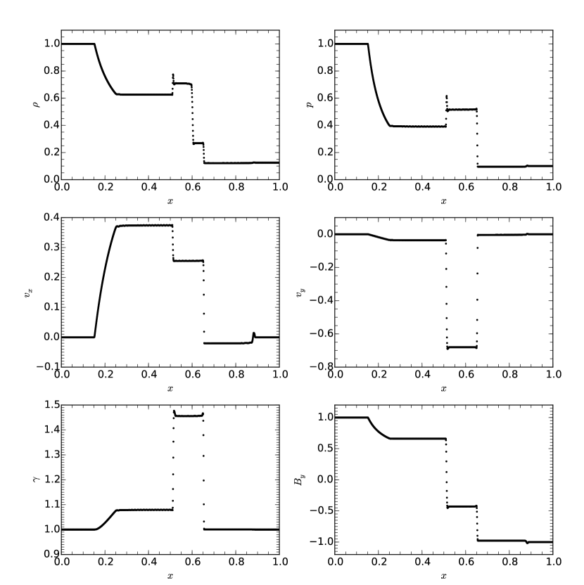
Figure 2.— Result for generalized Brio-Wu shock tube problem in RMHD regime. The fluid quantities are appropriate averages of the two fluids for comparison with published RMHD results.

Fig. 2 shows the numerical solution at $t=0.4$ for a pair plasma with $\mu_{p}=-\mu_{e}=10^{4}$. The number of grid points was 1600. Because the skin depth $\lambda_{p}=10^{-4}/\sqrt{\rho}$ was smaller than the grid size in the entire box, the solution agreed quite well with the RMHD result presented in the literature.

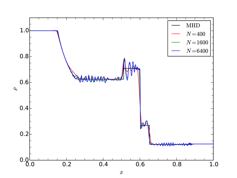
Figure 3.— Comparison of total density profiles at $t=0.4$ obtained with different resolutions for generalized Brio-Wu shock tube problem. A pair plasma is assumed. Three different numerical solutions with different numbers of grid points are shown, along with a reference solution corresponding to the RMHD regime.

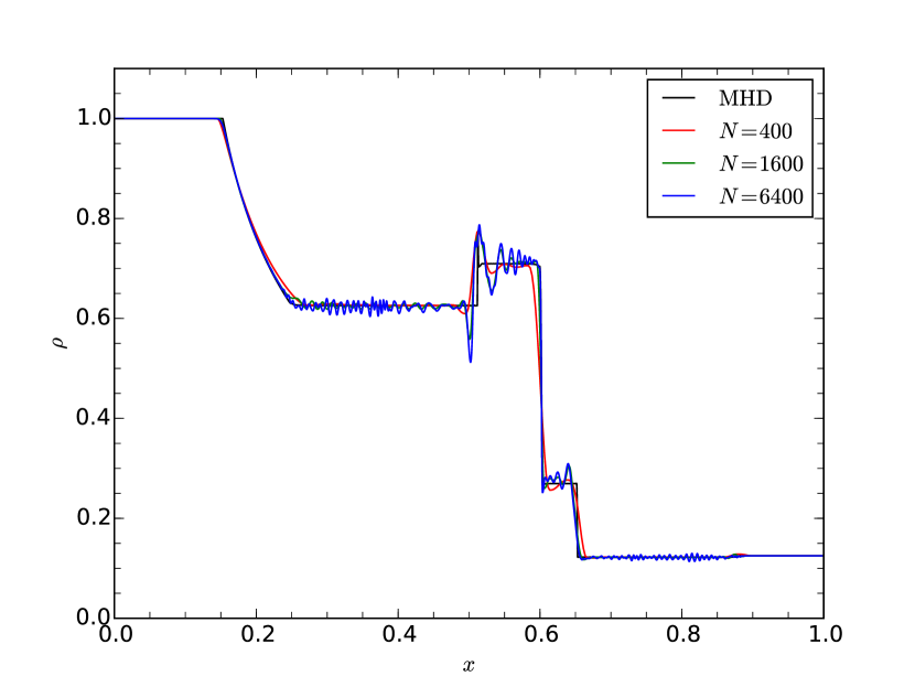
Figure 4.— Same as Fig. 3 but for an electron-proton plasma $m_{p}/m_{e}=100$.

On the other hand, Fig. 3 and 4 show results for $\mu_{p}=10^{3}$ with $m_{p}/m_{e}=1$ and $100$, respectively. The total density profiles obtained with three different resolutions are shown in each panel: $N=400$ (red), $1600$ (green), $6400$ (blue). A reference solution corresponding to the RMHD limit ($\mu_{p}=10^{5},m_{p}/m_{e}=1,N=6400$) is also shown with a black line for comparison. The grid size in the lowest resolution run was slightly larger than the skin depth. Thus, the numerical solutions roughly agreed with the RMHD prediction, although discontinuities were smeared out by numerical dissipation. As increasing the resolution, dispersive waves due to the two-fluid effect clearly appeared in the solutions. The results for a pair plasma and an electron-proton plasma are qualitatively the same. The most noticeable difference is the dip in density ahead (to the left) of the slow compound wave at $x\simeq 0.5$ in the electron-proton case. A similar structure was also observed in the non-relativistic case (Hakim et al., 2006; Amano, 2015).

4.3. Orszag-Tang vortex

The Orszag-Tang vortex problem has been used as a benchmark problem for multidimensional MHD codes. Although the problem starts from a smooth profile, the solution involves complicated multidimensional discontinuities. This possibly produces non-negligible numerical error in the divergence-free condition $\nabla\cdot\mathbf{B}=0$, which may lead to collapse of the numerical simulation. Here we adopt a relativistic analog of the problem to demonstrate that our code is capable of describing complex multidimensional flows involving discontinuities without numerical difficulty.

The initial condition was the same as that used in Beckwith & Stone (2011). The simulation domain was a 2D unit square $0\leq x\leq 1,0\leq y\leq 1$ with the periodic boundary condition applied in both directions. The initial condition for the density $\rho=\Gamma^{2}/4\pi$, and pressure $p=\Gamma/4\pi$ were uniform, where we used $\Gamma=5/3$. The three velocity and the magnetic field were initialized as follows:

$$V_{x}=-V_{0}\sin\left(2\pi y\right),\quad V_{y}=V_{0}\cos\left(2\pi x\right)$$ (69)

$$B_{x}=-B_{0}\sin\left(2\pi y\right),\quad B_{y}=B_{0}\sin\left(4\pi x\right),$$ (70)

where $V_{0}=1/2$ and $B_{0}=1/\sqrt{4\pi}$, respectively. We assumed a pair plasma $\mu_{p}=-\mu_{e}=10^{3}$, which makes the skin depth smaller than the grid size. However, the effective skin depth including the effect of the relativistic temperature was found to be comparable to the grid size in the numerical solution. Therefore, the result would be modified slightly from the RMHD solution by the two-fluid effect. The out-of-plane magnetic field was zero $B_{z}=0$, whereas $V_{p,z}=-V_{e,z}$ was finite so as to satisfy Ampere’s law in the initial condition. The corresponding four velocity was given by

$$u_{p,z}=-u_{e,z}=\frac{4\pi cB_{0}}{\mu_{p}\rho}\left(\cos\left(4\pi x\right)+\frac{1}{2}\cos\left(2\pi y\right)\right)$$ (71)

The in-plane components of the velocity for each fluid may be taken to be equal: $V_{p,x}=V_{e,x},V_{p,y}=V_{e,y}$. The electric field was initialized by $\mathbf{E}=-\mathbf{V}/c\times\mathbf{B}$. Note that the initial condition satisfies not only $\nabla\cdot\mathbf{B}=0$, but also $\nabla\cdot\mathbf{E}=0$, the latter is consistent with the charge neutrality $\mu_{p}\rho_{p}+\mu_{e}\rho_{e}=0$.

The numerical solution with a $200\times 200$ mesh at $t=1$ is shown in Fig. 5 for the density, gas pressure, magnetic pressure, and bulk Lorentz factor, respectively. A CFL number of 0.2 was used. The density and gas pressure agreed quite well with the published RMHD results (Beckwith & Stone, 2011), whereas small scale features in the magnetic pressure were slightly different due to the appearance of the two-fluid effect.

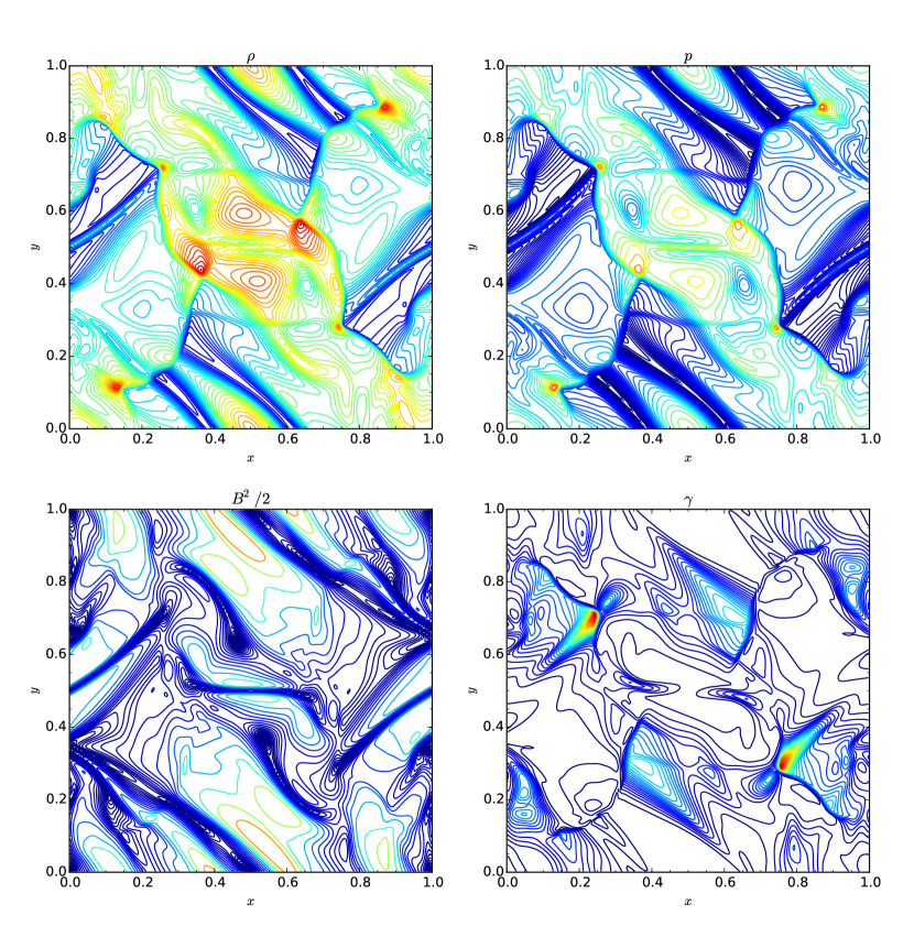
Figure 5.— Results for Orszag-Tang vortex problem at $t=1.0$. The total density (top left), gas pressure (top right), magnetic pressure (bottom left), and bulk Lorentz factor (bottom right) are shown. In each panel, 40 contours are drawn in the ranges $5.0\times 10^{-2}$ to $5.0\times 10^{-1}$ for the density, $2.0\times 10^{-2}$ to $6.0\times 10^{-1}$ for the gas pressure, $3.0\times 10^{-6}$ to $3.0\times 10^{-1}$ for the magnetic pressure, and $1.01$ to $2.0$ for the Lorentz factor, respectively. The contours are evenly spaced in linear scale for the density and Lorentz factor, and in logarithmic scale for the gas pressure and magnetic pressure.

4.4. Strong cylindrical explosion

The strong cylindrical explosion in a magnetized uniform medium has been a stringent benchmark problem to test the robustness of a numerical scheme. We adopt the relativistic version described in Komissarov (1999). The simulation box was a 2D square domain: $-6\leq x\leq+6,-6\leq y\leq+6$. We used a $200\times 200$ mesh. Initially, the density and pressure in the central region $r<0.8$ (where $r=\sqrt{x^{2}+y^{2}}$ is the distance from the origin) were $\rho_{in}=10^{-2}$ and $p_{in}=1.0$, which were respectively higher than those in the uniform surrounding medium $\rho_{out}=10^{-4}$, $p_{out}=5\times 10^{-4}$. Both the density and pressure linearly decreased from the values of the inside ($\rho_{in},p_{in}$) to the outside ($\rho_{out},p_{out}$) in the range $0.8\leq r\leq 1$. The plasma was initially at rest and the electric field was zero. The initial magnetic field was in the $x$ direction: $B_{x}=B_{0}$. The results of two runs with different initial magnetic field strength $B_{0}$ are shown below. We considered a pair plasma and the charge-to-mass ratio was chosen to be $\mu_{p}=-\mu_{e}=10^{3}$. This gives a skin depth of $\lambda_{p}=10^{-3}/\sqrt{\rho}$, which is slightly larger than the grid size ($\Delta x=\Delta y=0.06$) in the surrounding uniform medium ($\lambda_{p}=0.1$ for $\rho=10^{-4}$). Simulations were run with a CFL number of 0.1.

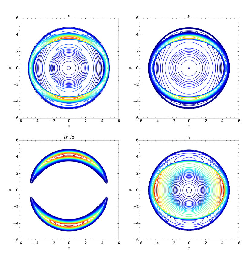
Figure 6.— Results for strong cylindrical explosion at $t=4.0$ in a weakly magnetized medium ($B_{0}=0.1$). The format is the same as Figure 5. In each panel, 30 contours are drawn in the ranges $8.0\times 10^{-5}$ to $8.0\times 10^{-4}$ for the density, $4.0\times 10^{-4}$ to $4.0\times 10^{-2}$ for the gas pressure, $7.0\times 10^{-3}$ to $7.0\times 10^{-2}$ for the magnetic pressure, and $1.01$ to $4.0$ for the Lorentz factor, respectively. The contours are evenly spaced in logarithmic scale.

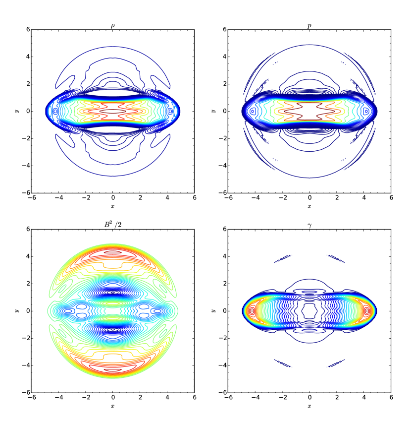
Figure 7.— Results for strong cylindrical explosion at $t=4.0$ in a strongly magnetized medium ($B_{0}=1.0$). The format is the same as Figure 5. In each panel, 30 contours are drawn in the ranges $5.0\times 10^{-5}$ to $2.0\times 10^{-3}$ for the density, $1.0\times 10^{-4}$ to $1.0\times 10^{-1}$ for the gas pressure, $3.0\times 10^{-1}$ to $7.0\times 10^{-1}$ for the magnetic pressure, and $1.01$ to $3.0$ for the Lorentz factor, respectively. The contours are evenly spaced in logarithmic scale.

Fig. 6 shows the result for a weakly magnetized medium $B_{0}=0.1$. A strong shock expanded roughly symmetrically into the surrounding medium. The numerical solution was quite similar to the RMHD result. The maximum Lorentz factor was $\gamma_{\rm max}\simeq 3.95$. On the other hand, Fig. 7 shows the result for a strongly magnetized medium $B_{0}=1.0$. In this case, the magnetic field in the surrounding medium was so strong that the inner structure was significantly modified. As a result, the expansion was primarily in the direction parallel to the ambient magnetic field. The maximum Lorentz factor in this case reached $\gamma_{\rm max}\simeq 3.00$. In general, this problem is known to be a stringent problem for which many RMHD codes would fail unless ad hoc changes were introduced in the code. Nevertheless, our code is able to keep track of the evolution of the problem without any numerical tricks.

4.5. Self-similar current sheet

So far we have considered test problems without resistivity. The resistive effect can be tested using the problem first presented in Komissarov (2007). We consider a 1D current sheet that involves only variation in the $B_{y}$ component. When the magnetic pressure is much smaller than the constant gas pressure, the evolution of the magnetic field in a resistive medium may be approximated by the diffusion equation:

$$\frac{\partial B_{y}}{\partial t}-D\frac{\partial^{2}B_{y}}{\partial x^{2}}=0,$$ (72)

where the diffusion coefficient is given in terms of resistivity by $D=\eta c^{2}$. A self-similar solution suggested by Komissarov (2007) is given as follows

$$B_{y}(x,t)=B_{0}\,{\rm erf}\left(\frac{x}{2\sqrt{Dt}}\right),$$ (73)

where ${\rm erf}(x)$ is the error function.

We set up the initial condition using the analytic solution at $t=1$ with $B_{0}=1$ and $\eta c^{2}=D=0.01$ in a 1D computational domain $-1.5\leq x\leq+1.5$ with 200 grid points. We used the conducting wall boundary condition. The charge-to-mass ratios were taken as $\mu_{p}=-\mu_{e}=10^{3}$. This gives the skin depth of $\lambda_{p}=10^{-3}/\sqrt{\rho}$, which is much smaller than the grid spacing $\Delta x=1.5\times 10^{-2}$. One can thus expect that the RTFED equations should reproduce the RMHD result.

The $x$ and $y$ components of the magnetic field and the electric field were zero. The density and pressure were uniform $\rho=1$ and $p=50$. The $x$ and $y$ components of velocity were zero, whereas the $z$ component was initialized by

$$u_{p,z}=-u_{e,z}=\frac{cB_{0}}{\mu_{p}\rho\sqrt{\pi D}}\exp\left(-\frac{x^{2}}{4D}\right).$$ (74)

This gives the conduction current that is consistent with Ampere’s law.

Fig. 8 shows the numerical solution at $t=9$ in parallel with the analytic prediction. A CFL number of 0.5 was used for the simulation. The two solutions were essentially indistinguishable. This indicates that our choice of the friction term can reproduce the resistive RMHD result.

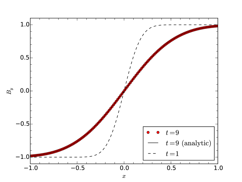
Figure 8.— Comparison between numerical and analytical solutions for self-similar current sheet problem. The profiles at $t=9$ are shown with dots for the numerical solution, and in a solid line for the analytic solution, respectively. The initial condition ($t=1$) is shown with dashed line.

4.6. Resistive perpendicular shock

This test problem first proposed by Barkov et al. (2014) deals with a fast magnetosonic shock propagating across the magnetic field in the two-fluid regime. At a scale length comparable to the skin depth, a shock wave in the two-fluid approximation in general involves a dispersive wave train either in the upstream or downstream of the shock. For a perpendicular fast-mode shock, the wave train appears only in the downstream because the group velocity $d\omega/dk$ is a decreasing function of $k$. The amplitude of the wave train gradually decreases due to dissipation as increasing the distance from the shock. In the presence of a finite resistivity, one can check the convergence of the numerical solution by increasing the resolution beyond the resistive scale length.

Table 3Left and right states for resistive perpendicular shock problem.

Parameter	Left state	Right state
$\rho$	1.0	2.059639
$\gamma$	10.0	4.933298
p	0.1	0.3420819
$B_{y}$	60	60.9648752

The simulation setup was essentially the same as that of the generalized Brio-Wu problem discussed in section 4.2, except for different initial left and right states. The initial left and right states were determined by solving numerically the Rankine-Hugoniot relations for a perpendicular RMHD shock with $\Gamma=4/3$, and are given in Table 3. The normal flow velocity and the $z$ component of electric field were respectively given by $u_{x}=\sqrt{1+\gamma^{2}}$ and $E_{z}=-u_{x}B_{y}/\gamma c$, whereas other components of vector quantities were initialized by zero. We considered a pair plasma with a charge-to-mass ratio of $\mu_{p}=-\mu_{e}=200$, which gives $\lambda_{p}=5\times 10^{-3}/\sqrt{\rho}$. We adopted a constant resistivity of $\eta=2.5\times 10^{-3}$, corresponding to a normalized frictional relaxation time scale of $\tau_{f}=1/\omega_{p}\eta=0.2$. The magnetization parameter in the upstream (left) medium in this setup becomes $\sigma_{e}=\sigma_{p}=72$. Therefore, the problem deals with a strongly magnetized plasma. This set of parameters is very similar to the case 1 of the problem discussed in section 4.3 of Barkov et al. (2014). However, our setup was not exactly the same because we could not reproduce their results: this is probably because of some errors in their description of the initial condition.

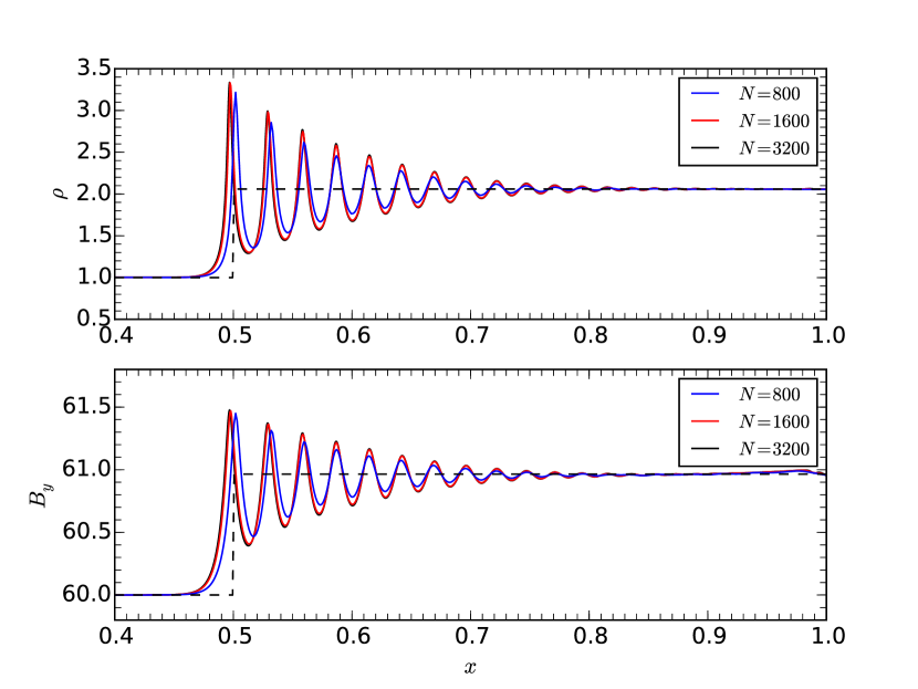
Figure 9.— Results for resistive perpendicular shock problem. The density (top) and $y$ component of the magnetic field (bottom) profiles are shown at $t=0.5$. The results with three different resolutions are shown with solid lines with different colors (blue, red, and black for $N=800,1600,3200$, respectively). The dashed lines show the initial condition corresponding to the RMHD Rankine-Hugoniot relations.

In Fig. 9, the density and magnetic field profiles at $t=0.5$ are shown for three different resolutions: $N=800,1600,3200$. A CFL number of 0.2 was used in every run. Because the initial condition satisfied the Ranking-Hugoniot relations, the shock structure was stationary in the simulation frame. The shock transition did not involve a discontinuous subshock but it did exhibit a laminar profile with a trailing wave train structure as shown by Barkov et al. (2014). It appeared that the solution with $N=1600$ almost coincides with that of $N=3200$, indicating that numerical convergence was achieved at this resolution. In contrast, when the physical resistivity was turned off, we did not observe the convergence of the numerical solution. This is because “resistive” dissipation always occurs at the grid scale. In any case, there was no numerical stability issue even without finite resistivity.

4.7. Magnetic reconnection

Our final test problem is magnetic reconnection for a strongly magnetized electron-proton plasma. Previous simulation studies of relativistic magnetic reconnection in the two-fluid regime have been presented only for a pair plasma. On the other hand, it is well known that magnetic reconnection becomes efficient in a thin current sheet whose thickness is on the order of ion skin depth in a non-relativistic electron-proton plasma. Here we demonstrate that essentially the same argument applies to the relativistic regime and fast magnetic reconnection is realized.

The simulation setup was an extension of a non-relativistic GEM (Geospace Environment Modeling) magnetic reconnection problem (e.g., Birn et al., 2001). The initial magnetic field and proper number density profiles were given by

$$B_{x}=B_{0}\tan\left(y/d\right),B_{y}=B_{z}=0,$$ (75)

and

$$n=n_{0}{\rm sech}^{2}\left(y/d\right)+n_{\rm bg}$$ (76)

respectively. The number density was assumed to be the same between the species. The system is characterized by the magnetization parameter $\sigma_{s}=B_{0}^{2}/n_{0}m_{s}c^{2}$. It is readily seen that the Alfven speed is approximately given by $v_{A}/c\simeq\sqrt{\sigma_{p}/(1+\sigma_{p})}$ for $m_{p}/m_{e}\gg 1$. The relativistic effect thus becomes important for magnetic reconnection in a strongly magnetized plasma $\sigma_{p}\gtrsim 1$. The initial temperature was given by $T_{s}/m_{s}c^{2}=\sigma_{s}/4$, which is consistent with the pressure balance condition for an equal temperature plasma $T_{p}=T_{e}$. Similarly, we assumed that the initial current is carried equally by the two species. This leads to the $z$ component of four velocity

$$u_{z,p}=-u_{z,e}=\frac{c}{2ed}\frac{B_{0}{\rm sech}^{2}(y/d)}{n_{0}{\rm sech}^{2}(y/d)+n_{\rm bg}},$$ (77)

for consistency with Ampere’s law. Other components of velocity were initialized by zero. Notice that because the Lorenz factors are the same between the species with this setup, the charge neutrality $\nabla\cdot\mathbf{E}=0$ in the initial condition is automatically satisfied. We thus assumed that the electric field was initially zero everywhere in the simulation box. In addition, to initiate magnetic reconnection, the magnetic field was perturbed by introducing the out-of-plane vector potential of the form

$$\Phi=\alpha B_{0}\cos\left(\frac{\pi x}{L}\right)\cos\left(\frac{\pi y}{L}\right),$$ (78)

where $L$ is the system size in $y$ direction and $\alpha=0.1$ is the amplitude of perturbation. More specifically, the two-dimensional computational domain $-L\leq x\leq+L$, $-L/2\leq y\leq+L/2$ was used. The number of grids in $x$ and $y$ directions were $2N$ and $N$, respectively. Thus, the grid sizes in each direction were the same $\Delta x=\Delta y$.

We adopt a normalization such that $c=m_{p}=n_{0}=1$ and $B_{0}=1/e=\sqrt{\sigma_{p}}$. With this normalization, time and length are measured in units of $\Omega_{c,p}^{-1}=(eB_{0}/m_{p}c)^{-1}$, and $c/\Omega_{c,p}$, respectively. A system size of $L/c/\Omega_{c,p}=12.8$, and a thickness of the current sheet of $d/c/\Omega_{c,p}=1$ were used. The boundary condition in the $x$ direction was periodic, whereas the conducting wall boundary condition was used in the $y$ direction. A time step of $\Omega_{c,p}\Delta t=10^{-3}$ was used for all the simulations shown below.

In the following, we show simulation results obtained with $m_{p}/m_{e}=25$, $\sigma_{p}=1.0$, $\sigma_{e}=25.0$. A background density of $n_{\rm bg}/n_{0}=0.2$ was used. In such a strongly magnetized current sheet, one has to take into account the effective inertia increase due to relativistic temperature. Consequently, the effective magnetization ratios become $\bar{\sigma}_{p}=\sigma_{p}/h_{p}=1/2$ and $\bar{\sigma}_{e}=\sigma_{e}/h_{e}=25/26$, respectively. Therefore, the Alfven speed was roughly 57% of the speed of light. We used a constant resistivity of $\eta c^{2}=0.01$. Time development of the normalized reconnected magnetic flux calculated by

$$\psi(t)=\frac{1}{2B_{0}}\int_{-L}^{L}\|B_{y}(x,y=0,t)\|dx$$ (79)

is shown in Fig. 10 for three runs with increasing resolutions: $N=128,256,512$. All three runs exhibited almost the same evolution. In particular, the results are almost indistinguishable up to $\Omega_{c,p}t\simeq 70$. In the late phase, the interaction between fast reconnection outflows and a plasmoid produced complicated structures involving discontinuities, which is probably the main reason for the slight deviation. The reconnection rate defined as the inflow speed toward the neutral sheet in units of Alfven speed $v_{\rm in}/v_{A}$ was estimated from the slope of the reconnected flux. The peak reconnection rate reached as high as $\sim 0.13$ at $\Omega_{c,p}t\simeq 62$. Similar reconnection rates are typically observed in Hall-MHD simulations for a non-relativistic electron-proton plasma.

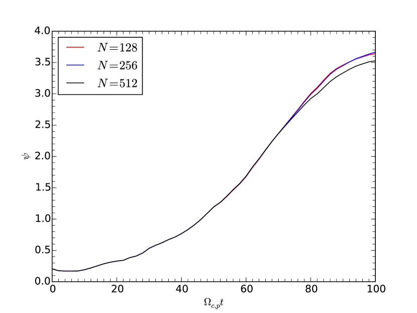
Figure 10.— Time development of reconnected magnetic flux for three runs with different resolutions $N=128,256,512$.

Fig. 11 and 12 show two snapshots at $\Omega_{c,p}t=40,80$ for the total mass density $\rho$, out-of-plane magnetic field $B_{z}$, $x$ component of four velocity for protons $u_{p,x}$ and electrons $u_{e,x}$, respectively. The reconnection occurred around the origin from which fast bipolar outflows were ejected both in the positive and negative $x$ directions. In Fig.11, we can clearly see the quadrupolar out-of-plane magnetic field $B_{z}$ around the X-point generated by the Hall effect. The outflow speed for protons was slower than electrons, indicating the decoupling between the species. At a later time, the outflow is accelerated even further. The ion outflow speed reached as high as the Alfven speed, whereas the electron outflow was accelerated essentially to the speed of light.

Although these qualitative features are essentially unchanged from the non-relativistic counterpart, there are quantitative differences. For instance, the observed magnitude of $B_{z}$ at early times was much smaller, which is somehow to be expected in the relativistic regime. The electron fluid had an increased effective inertia due to relativistic temperature $T_{e}/m_{e}c^{2}=6.25$, whereas the same effect was less important for protons $T_{p}/m_{p}c^{2}=0.5$. Consequently, the ratio of effective inertia between protons and electrons was reduced to $m_{p}(1+4T_{p}/m_{p}c^{2})/m_{e}(1+4T_{e}/m_{e}c^{2})\sim 1.9$ (where $\Gamma=4/3$ was used). This made the decoupling of the dynamics between the two fluids becomes relatively weak, resulting in the reduced amplitude of Hall magnetic field. Therefore, in an extreme situation $\sigma_{p}\gg m_{p}/m_{e}$, we expect that the dynamics will essentially become the same as that in a pair plasma as long as the temperatures of the two species remain the same. A more detailed study will be presented elsewhere in the future.

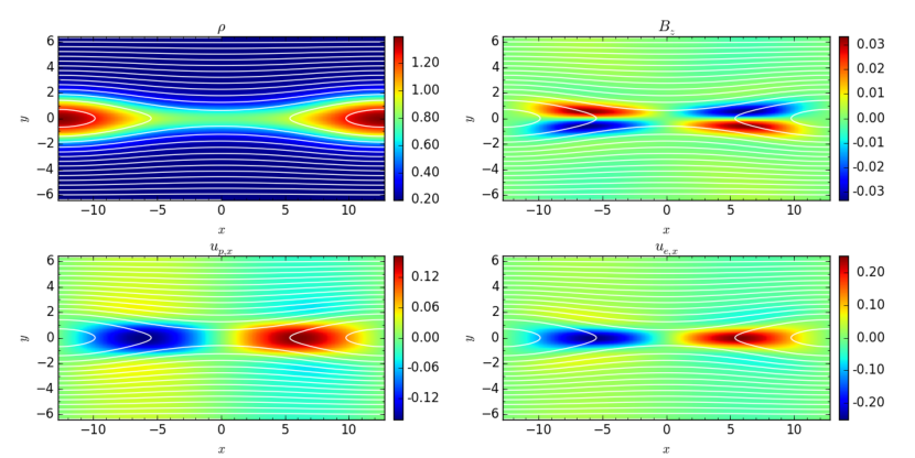
Figure 11.— Result for magnetic reconnection problem at $\Omega_{c,p}t=40$. The total mass density $\rho$ (top left), out-of-plane magnetic field $B_{z}$, $x$ component of four velocity for protons $u_{p,x}$ (bottom left), and electrons $u_{e,x}$ (bottom right) are shown. White contours represent the magnetic field lines.

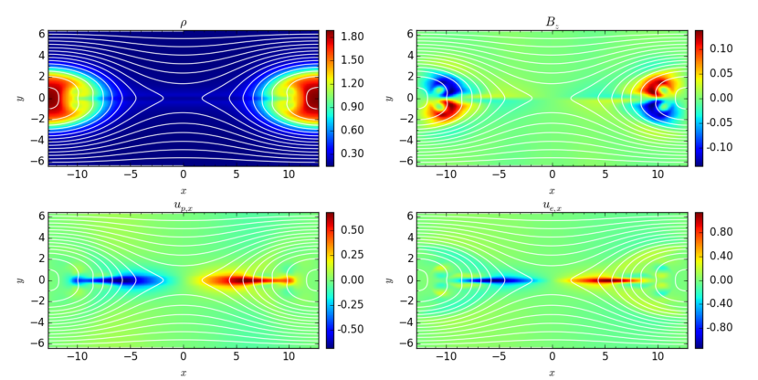
Figure 12.— Same as Fig. 11 but for $\Omega_{c,p}t=80$.

5. Conclusions

In this paper, we have discussed the relativistic two-fluid electrodynamics (RTFED) equations, which are an extension of relativistic magnetohydrodynamics (RMHD). The advantage of the RTFED model is obviously its capability for a wider range of applications. In contrast to RMHD, there is no inherent difficulty for dealing with a region where the local electric field is larger than the magnetic field, which may become important for extreme environments in high energy astrophysics. Also, it is easy to implement a finite resistivity without suffering from the singularity at infinite conductivity. The resistivity (or the friction term) introduced in this paper reduces to the one used in current generation resistive RMHD codes in the long wavelength limit. This fact remains valid regardless of the proton-to-electron mass ratio, which makes it possible to investigate the resistive effect in not only a pair plasma but also an electron-proton plasma.

A 3D simulation code solving the RTFED equations has been described. The code achieves overall second-order accuracy for smooth profiles. If the grid size is taken to be large compared to the skin depth, the RMHD shocks/discontinuities are captured without appreciable numerical oscillation. Furthermore, dispersive waves arising from the two-fluid effect are correctly described in cases where sufficient resolution is available. The numerical algorithm presented here guarantees that the two divergence constraints for the electromagnetic field are preserved up to machine precision.

It is also possible to extend the code to higher order. Indeed, Balsara et al. (2016) have presented up to a fourth-order accurate finite volume implementation for the RTFED equations. They have also invented a novel and more consistent reconstruction scheme of the electric field that satisfies Gauss’ law over the entire control volume. Alternatively, one may also adopt a finite difference approach, in which case a higher-order reconstruction/interpolation can be applied in a dimension-by-dimension manner. Note that, even in this case, it is possible to construct a scheme that exactly preserves the divergence constraints (e.g., Del Zanna et al., 2007).

To be fair, there is one critical disadvantage in the RTFED equation. Because it includes high-frequency plasma waves as eigenmodes even in the long wavelength limit, the numerical stability inevitably requires a small time step to resolve the plasma frequency. This is the most serious obstacle for the model when application to macroscopic phenomena (in the presence of a dense plasma) is considered. In these situations, the dynamical time scale and the inverse plasma frequency will differ by orders of magnitude. A naive way to resolve the issue is to use an implicit time integration scheme (e.g., Kumar & Mishra, 2012; Balsara et al., 2016). Indeed, because the high-frequency waves in the long wavelength limit are non-propagating, the scheme can be made locally implicit. This is advantageous because it will not require communications with neighboring processors in parallelization on a distributed memory system. It may also be possible to utilize analytic solutions for such high-frequency waves combined with the operator splitting technique if the wave amplitude remains sufficiently small.

Another numerical issue, although less important than the one above, is associated with the use of the simplified Riemann solver. Because the maximum phase speed in the RTFED equations is always given by the speed of light, it may introduce excessive numerical dissipation in situations where the RMHD characteristics have only non-relativistic speeds. In a sense, if the dynamical time scale is much less than the light transit time, one may think that the dynamics of the plasma are decoupled from the electromagnetic wave propagation. In principle, taking advantage of the decoupling, it would be possible to construct a more sophisticated Riemann solver that resolves the internal structure of the Riemann fan. This allows one to obtain higher accuracy both in non-relativistic and relativistic regions at the same time.

Despite the numerical issues raised above, given the potential of the RTFED equations, it is important to continue investigating of numerical methods to overcome the weak points. This will certainly extend the applicability of the model in the field of high energy astrophysics.

Appendix A Finite Amplitude Circularly Polarized Wave

It has been known that there exists an analytic solution to a finite amplitude circularly polarized waves propagating along the ambient magnetic field for the relativistic cold two-fluid plasma equations (Kennel & Pellat, 1976). Because it does not involve density perturbations, it is relatively easy to include a finite temperature effect, as we demonstrate below.

We consider a magnetized plasma with a background magnetic field $\mathbf{B}=B_{0}\mathbf{e}_{x}$. The density, and temperature are assumed to be constant. On average (i.e, in the absence of transverse perturbation), the plasma is at rest in the laboratory frame, so that the flow velocity along the magnetic field is always zero $u_{x}=0$. The homogeneity in density implies that the longitudinal electric field is also zero $E_{x}=0$. Now it is convenient to introduce the following definitions for transverse perturbations:

$$B_{\perp}=B_{y}-iB_{z},\quad E_{\perp}=E_{y}-iE_{z},\quad u_{s,\perp}=u_{s,y}-iu_{s,z}.$$ (A1)

Because there is no longitudinal perturbation, only the transverse components of the equation of motion are non-trivial:

$$\frac{\partial}{\partial t}\left(\rho_{s}h_{s}\gamma_{s}u_{s,y}\right)=\mu_{s}\rho_{s}\gamma_{s}\left(E_{y}+\frac{u_{s,z}}{\gamma_{s}c}B_{0}\right),$$ (A2)

$$\frac{\partial}{\partial t}\left(\rho_{s}h_{s}\gamma_{s}u_{s,z}\right)=\mu_{s}\rho_{s}\gamma_{s}\left(E_{z}-\frac{u_{s,y}}{\gamma_{s}c}B_{0}\right),$$ (A3)

where $h_{s}$ is the specific enthalpy defined by Eq. (4), representing an inertia increase due to a relativistically hot temperature. In the absence of longitudinal perturbation, $h_{s}$ becomes just a constant, indicating that the effect of finite temperature may be included by simply replacing the mass $m_{s}$ of a cold fluid by $m_{s}h_{s}$.

Notice that, for circularly polarized modes, the Lorentz factor of the fluid due to particle quiver motion is constant. Therefore, it can be put outside of the temporal derivative, yielding

$$\frac{\partial}{\partial t}u_{s,\perp}=\frac{\mu_{s}}{h_{s}}E_{\perp}+i\frac{\bar{\Omega}_{c,s}}{\gamma_{s}}u_{s,\perp},$$ (A4)

where $\bar{\Omega}_{c,s}=\mu_{s}B_{0}/h_{s}c$ is the effective cyclotron frequency for particle species $s$.

Now we consider a monochromatic wave solution of the form $u_{s,\perp}=\tilde{u}_{s,\perp}\exp\left(ikx-i\omega t\right)$. With this definition, a solution in the domain $\omega>0,k>0$ corresponds to a right-hand circularly polarized mode propagating in the positive $x$ direction. Similarly, we also define $\tilde{E}_{\perp},\tilde{B}_{\perp}$ as the wave amplitude. Eq. (A4) then becomes

$$\tilde{u}_{s,\perp}=\frac{i}{\omega+\bar{\Omega}_{c,s}/\gamma_{s}}\frac{\mu_{s}}{h_{s}}\tilde{E}_{\perp},$$ (A5)

whereas we have from Maxwell’s equations

$$\left(1-\frac{k^{2}c^{2}}{\omega^{2}}\right)\tilde{E}_{\perp} =-\frac{i}{\omega}\sum\mu_{s}\rho_{s}\tilde{u}_{s,\perp},$$ (A6)

$$\tilde{E}_{\perp} =i\frac{\omega}{kc}\tilde{B}_{\perp}.$$ (A7)

Combining Eqs. (A5) and (A6), one obtains the dispersion relation:

$$\omega^{2}-k^{2}c^{2}-\sum\gamma_{s}\bar{\omega}_{p,s}^{2}\frac{\omega}{\gamma_{s}\omega+\bar{\Omega}_{c,s}}=0,$$ (A8)

where $\bar{\omega}_{p,s}^{2}=\mu_{s}^{2}\rho_{s}/h_{s}$ is the effective proper plasma frequency. Notice that, however, the above dispersion relation includes the Lorentz factors $\gamma_{s}$ for each fluid, which are yet unknown at this point.

To obtain the Lorentz factor, one may eliminate the electric field from Eqs. (A5) and (A7), yielding

$$\frac{\tilde{u}_{s,\perp}}{c}=-\gamma_{s}\frac{\bar{\Omega}_{c,s}}{\gamma_{s}\omega+\bar{\Omega}_{c,s}}\frac{\omega}{kc}\frac{\tilde{B}_{\perp}}{B_{0}}.$$ (A9)

Squaring the equation and using $\gamma_{s}^{2}=1+\tilde{u}_{\perp}^{2}/c^{2}$, we get the following equation:

$$\gamma_{s}^{4}+2\frac{\bar{\Omega}_{c,s}}{\omega}\gamma_{s}^{3}+\left(\frac{\bar{\Omega}_{c,s}^{2}}{\omega^{2}}\left(1-\frac{\omega^{2}}{k^{2}c^{2}}\xi^{2}\right)-1\right)\gamma_{s}^{2}-2\frac{\bar{\Omega}_{c,s}}{\omega}\gamma_{s}-\frac{\bar{\Omega}_{c,s}^{2}}{\omega^{2}}=0,$$ (A10)

where the wave magnetic field amplitude normalized to the background is denoted by $\xi=\tilde{B}_{\perp}/B_{0}$,

In summary, a finite amplitude circularly polarized wave solution for a given set of $(k,\xi)$ is obtained by iteratively searching for a solution $(\omega,\gamma_{p},\gamma_{e})$ that simultaneously satisfies the three equations: Eq.(A8) and (A10) for each fluid. In practice, one may adopt a simplified numerical procedure as explained below. Given an initial guess ($\omega,\gamma_{p},\gamma_{e}$), we first solve Eq. (A10) independently for a given $\omega$. Then, the dispersion relation (A8) is solved for given $(\gamma_{p},\gamma_{e})$. The solution is obtained by iterating the whole procedure. We find that even with this simplified iteration procedure, the solution converges rather quickly.

For a fixed $k>0$, the dispersion relation has two solutions in the region $\omega>0$; a subluminal $(\omega/k<c)$ Alfvén mode, and a superluminal $(\omega/k>c)$ electromagnetic mode. Therefore, by starting from a small $\omega$ as an initial guess, the solution will converge to the subluminal mode. Conversely, a larger initial guess of $\omega$ will converge to the superluminal mode. A left-hand circularly polarized wave solution can also be obtained as a negative frequency root $\omega<0$ of the same equation.

Notice that because the Lorentz factors of the two fluids are different, the proper number densities must also be different to satisfy the charge neutrality condition

$$\sum\mu_{s}\rho_{s}\gamma_{s}=\sum e_{s}n_{s}\gamma_{s}=0.$$ (A11)

Namely, it is the lab frame number density that must be equal between the species. This condition is indeed necessary so that the dispersion relation reduces to the Alfvén wave of RMHD in the low frequency limit $\omega\ll\bar{\Omega}_{c,s}/\gamma_{s}$.

It is also worth noting that, for a given amplitude $\xi$, there exists a critical wavenumber beyond which the Alfvén mode does not exist (Hada et al., 2004). This occurs due to increased particle inertia by relativistic quiver motion, which decreases the effective cyclotron frequency. For numerical benchmark problems, this does not pose any difficulty by using a sufficiently small amplitude and/or wavenumber.

References

- Amano (2015) Amano, T. 2015, Journal of Computational Physics, 299, 863
- Amano et al. (2014) Amano, T., Higashimori, K., & Shirakawa, K. 2014, Journal of Computational Physics, 275, 197
- Amano & Kirk (2013) Amano, T., & Kirk, J. G. 2013, ApJ, 770, 18
- Balsara (2001) Balsara, D. S. 2001, Journal of Computational Physics, 174, 614
- Balsara (2004) —. 2004, ApJS, 151, 149
- Balsara (2009) —. 2009, Journal of Computational Physics, 228, 5040
- Balsara (2010) —. 2010, Journal of Computational Physics, 229, 1970
- Balsara (2012) —. 2012, Journal of Computational Physics, 231, 7476
- Balsara et al. (2016) Balsara, D. S., Amano, T., Garain, S., & Kim, J. 2016, Journal of Computational Physics, 318, 169
- Balsara & Spicer (1999) Balsara, D. S., & Spicer, D. S. 1999, Journal of Computational Physics, 149, 270
- Barkov et al. (2014) Barkov, M., Komissarov, S. S., Korolev, V., & Zankovich, A. 2014, MNRAS, 438, 704
- Barkov & Komissarov (2016) Barkov, M. V., & Komissarov, S. S. 2016, MNRAS, 458, 1939
- Beckwith & Stone (2011) Beckwith, K., & Stone, J. M. 2011, ApJS, 193, 6
- Birn et al. (2001) Birn, J., et al. 2001, J. Geophys. Res., 106, 3715
- Coroniti (1990) Coroniti, F. V. 1990, ApJ, 349, 538
- Dai & Woodward (1998) Dai, W., & Woodward, P. R. 1998, Journal of Computational Physics, 142, 331
- Del Zanna et al. (2003) Del Zanna, L., Bucciantini, N., & Londrillo, P. 2003, A&A, 400, 397
- Del Zanna et al. (2007) Del Zanna, L., Zanotti, O., Bucciantini, N., & Londrillo, P. 2007, A&A, 473, 11
- Drenkhahn & Spruit (2002) Drenkhahn, G., & Spruit, H. C. 2002, A&A, 391, 1141
- Esirkepov (2001) Esirkepov, T. Z. 2001, Computer Physics Communications, 135, 144
- Evans & Hawley (1988) Evans, C. R., & Hawley, J. F. 1988, ApJ, 332, 659
- Gardiner & Stone (2005) Gardiner, T. A., & Stone, J. M. 2005, Journal of Computational Physics, 205, 509
- Hada et al. (2004) Hada, T., Matsukiyo, S., & Munoz, V. 2004, ArXiv Physics e-prints
- Hakim et al. (2006) Hakim, A., Loverich, J., & Shumlak, U. 2006, Journal of Computational Physics, 219, 418
- Hewett & Nielson (1978) Hewett, D. W., & Nielson, C. W. 1978, Journal of Computational Physics, 29, 219
- Kennel & Coroniti (1984) Kennel, C. F., & Coroniti, F. V. 1984, ApJ, 283, 694
- Kennel & Pellat (1976) Kennel, C. F., & Pellat, R. 1976, J. Plasma Phys., 15, 335
- Kirk & Skjæraasen (2003) Kirk, J. G., & Skjæraasen, O. 2003, ApJ, 591, 366
- Koide et al. (1999) Koide, S., Shibata, K., & Kudoh, T. 1999, ApJ, 522, 727
- Komissarov (1999) Komissarov, S. S. 1999, MNRAS, 303, 343
- Komissarov (2007) —. 2007, MNRAS, 382, 995
- Komissarov et al. (2007a) Komissarov, S. S., Barkov, M., & Lyutikov, M. 2007a, MNRAS, 374, 415
- Komissarov et al. (2007b) Komissarov, S. S., Barkov, M. V., Vlahakis, N., & Königl, A. 2007b, MNRAS, 380, 51
- Komissarov et al. (2009) Komissarov, S. S., Vlahakis, N., Königl, A., & Barkov, M. V. 2009, MNRAS, 394, 1182
- Kumar & Mishra (2012) Kumar, H., & Mishra, S. 2012, Journal of Scientific Computing, 52, 401
- Kurganov et al. (2001) Kurganov, A., Noelle, S., & Petrova, G. 2001, SIAM J. Sci. Comput., 23, 707
- Londrillo & Del Zanna (2000) Londrillo, P., & Del Zanna, L. 2000, ApJ, 530, 508
- Londrillo & Del Zanna (2004) —. 2004, Journal of Computational Physics, 195, 17
- Lyubarsky & Kirk (2001) Lyubarsky, Y., & Kirk, J. G. 2001, ApJ, 547, 437
- McKinney (2006) McKinney, J. C. 2006, MNRAS, 368, 1561
- Melatos & Melrose (1996) Melatos, A., & Melrose, D. B. 1996, MNRAS, 279, 1168
- Michel (1994) Michel, F. C. 1994, ApJ, 431, 397
- Minoshima et al. (2015) Minoshima, T., Hirose, S., & Sano, T. 2015, ApJ, 808, 54
- Mizuno et al. (2004) Mizuno, Y., Yamada, S., Koide, S., & Shibata, K. 2004, ApJ, 606, 395
- Nishikawa et al. (2005) Nishikawa, K.-I., Richardson, G., Koide, S., Shibata, K., Kudoh, T., Hardee, P., & Fishman, G. J. 2005, ApJ, 625, 60
- Rees & Gunn (1974) Rees, M. J., & Gunn, J. E. 1974, MNRAS, 167, 1
- Ryu et al. (1998) Ryu, D., Miniati, F., Jones, T. W., & Frank, A. 1998, ApJ, 509, 244
- Shu & Osher (1988) Shu, C.-W., & Osher, S. 1988, Journal of Computational Physics, 77, 439
- Srinivasan & Shumlak (2011) Srinivasan, B., & Shumlak, U. 2011, Physics of Plasmas, 18, 092113
- Takahashi et al. (2011) Takahashi, H. R., Kudoh, T., Masada, Y., & Matsumoto, J. 2011, ApJ, 739, L53
- Takamoto (2013) Takamoto, M. 2013, ApJ, 775, 50
- Tchekhovskoy et al. (2009) Tchekhovskoy, A., McKinney, J. C., & Narayan, R. 2009, ApJ, 699, 1789
- Thompson (1994) Thompson, C. 1994, MNRAS, 270, 480
- Toma & Takahara (2014) Toma, K., & Takahara, F. 2014, MNRAS, 442, 2855
- Watanabe & Yokoyama (2006) Watanabe, N., & Yokoyama, T. 2006, ApJ, 647, L123
- Zenitani et al. (2009a) Zenitani, S., Hesse, M., & Klimas, A. 2009a, ApJ, 696, 1385
- Zenitani et al. (2009b) —. 2009b, ApJ, 705, 907
- Zenitani et al. (2010) —. 2010, ApJ, 716, L214