A large eddy simulation (LES) study of inertial deposition of particles onto in-line tube-banks

Abstract

We study deposition and impact of heavy particles onto an in-line tube-banks within a turbulent cross flow through Lagrangian particle tracking coupled with an LES modelling framework. The flow Reynolds number based on the cylinder diameter $D$ and flow velocity between the gap of two vertically adjacent cylinders is $33960$. We examine the flow structures across the tube bank and report surface pressure characteristics on cylinders. Taking into account particle-wall impact and bounce, we study dispersion and deposition of three sets of particles ($St=0.35,0.086,0.0075$) based on $10^{7}$ particles tracked through the turbulent flow resolved by LES. The deposition efficiency for the three sets of particles are reported across the tube-banks. Positions of particle deposited onto tube-banks shows that significantly more of smaller particles deposit onto the back-side of the back-banks. This suggests that the smaller particles are easier to be entrained into the wake and impact onto the back-side of cylinders.

1 Introduction

Investigation of the deposition and impact of aerosol particles on heat exchangers is of significant importance to the design and operation of heat exchanger tube banks used in a wide range of industrial applications, i.e., civil advanced gas-cooled reactor (CAGR) boilers, oil-fired steam boilers of thermal power stations and process plants. In many safety cases involving dropped fuel in CAGRs a significant proportion of the activity will be associated with small aerosol particles. The main mechanisms by which aerosol particulates deposit and impact on wall surfaces include gradient/diffusion or free-flight theory , inertia deposition, interception, turbulent eddy-diffusion, Brownian diffusion and thermophoresis, gravitational setting, etc. The mechanisms that are responsible for the deposition of heavy particles in fully developed turbulent boundary layers are gradient/diffusion or free flight theory  ([1]) and by turbophoresis  ([2]) with turbulent eddy-diffusion  ([3]). However, under the conditions of high volume flow rate low pressure drop filtration, inertial impact becomes the dominant mechanism governing deposition among all the competing ones that contribute to the deposition of aerosol particulates on cylinder surfaces (see  [4, 5]).

There has been extensive research regarding the inertia deposition of heavy particles or droplets from flowing gas streams by impact on a single cylinder surfaces through theory and experiments. For example, Brun et al. [6] reported three impingement characteristics of water droplets on a cylinder surface, which are total rate of water droplet impingement, extend of droplet impingement zone and local distribution of impinging water on cylinder surface. The results on the collection efficiency of a cylinder in Brun et al. [6] were presented as a function of combining the Stokes and Reynolds number of droplets considered. This treatment was extended to use a generalized Stokes number to determine the collection efficiency of a cylinder for non-Stokesian particles by Israel and Rosner[7]. This generalized Stokes number is normally referred to as effective Stokes number and defined as

$$St_{\mathrm{eff}}=\psi(Re_{p})St,$$ (1)

where $\psi(Re_{p})$ is the non-Stokes drag correction factor and given by

$$\psi(Re_{p})=\frac{24}{Re_{p}}\int_{0}^{Re_{p}}\frac{1}{C_{D}(Re^{\prime})\,Re^{\prime}}\,\mathrm{d}Re^{\prime},$$ (2)

and

$$St=\frac{\rho_{p}d_{p}^{2}U_{o}}{18uD}.$$ (3)

More recently, the collection efficiency was examined through directly solving the incompressible Navier-Stokes equations coupled with the Lagrangian point particle tracking approach in a relatively low Reynolds number cross flow across a cylinder by Haugen et al.[8].

There are a number of numerical studies on the deposition and impact of heavy particles on tube-banks surfaces, and they focused on the two-dimensional simulations. Jun and Tabakoff[9] carried out a two-dimensional numerical simulation for a dilute particle laden laminar flow over in-line tube-banks in order to study particle impact and erosion of cylinders. Rebound phenomena of particles from cylinder surfaces were take into account as well in the above work. Bouris et al.[10] performed a two-dimensional large eddy simulation to evaluate alternate tube configurations for particle deposition rate reduction on heat exchanger tube bundles, in which an energy balance model was implemented to consider the adhesion or rebound of particles upon hitting upon the surface a tube. Tian et al.[11] made use of the two-dimensional RANS (Reynolds-averaged Navier-Stokes) modelling framework and Lagrangian particle tracking to study the characteristics of particle-wall collisions. An algebraic particle-wall collision and stochastic wall roughness model was also implemented by Tian et al. [11].

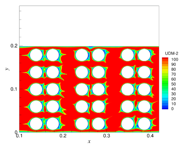
Figure 1: Contour of the $y^{+}$ value of each cell associated with its correspondingly nearest wall-adjacent cell face in a turbulent flow across in-line tube-banks. UDM-2 stands for $y^{+}$.

Engineering predictions of the deposition of heavy particles on bluff bodies depends primarily on the RANS. The methodology of three-dimensional RANS modelling frameworks coupled with a separate boundary layer model, which supplies fluctuating fluid velocity fluctuations seen by heavy particles, has been extended to study the prediction of deposition rates of heavy particles (e.g. [12, 13]) in complex geometries. Dehbi and Martin[14] further employed above mentioned method to study particulate flows around linear arrays of spheres and got good predicted deposition rates when compared against experimental measurements. However, for a turbulent flow across bluff bodies, e.g. spheres or cylinders, the salient feature of such a flow is that it has strongly unsteady, three-dimensional vortex shedding ([15]). This requires solving the Navier-Stokes equations with the time-dependent term, i.e. unsteady RANS (URAS) or LES, in order to resolve the unsteady phenomena of vortex shedding as accurately as possible. In this study, first a URAS simulation was carried out for a turbulent flow across in-line tube-banks. The approach presented in Dehbi[12] was used to determine the $y^{+}$ value of each cell associated with its correspondingly nearest wall-adjacent cell face. However, as shown in figure 1 for the contour of $y^{+}$ values of each cell associated with its correspondingly nearest wall-adjacent cell face, the boundary layer around every cylinder based on a threshold $y^{+}$ value $100$ possesses a irregular shape. This irregular boundary layer shape as a result of the unsteadiness of vortex shedding may make the methodology of RANS modelling framework combining with a supplying boundary model problematic.

LES has been convincingly demonstrated to be superior to unsteady RANS (URANS) in accurately predicting the flow and vortex dynamics of a turbulent cross-flow in a staggered ([16]) and in-line tube bundle ([17]). This is because LES is capable of providing the detailed large scales of flow structures, resolving a significant part of the vortex shedding physics and hence reducing the importance of modelling. The success of LES technique for single-phase turbulent flows across complex geometries has been explored to extend the technique to two-phase flows over complex geometries. Apte et al.[18] performed an LES study of particle-laden swirling flow in a coaxial-jet combustor. They demonstrated that results obtained from LES are significantly more accurate than the results by RANS applied for the same problem. Riber et al.[19] conducted a comparison study of numerical strategies for LES of particulate two-phase recirculating flows and observed that the dispersed phase is predicted more accurately by the Lagrangian point particle approach than the Eulerian approach. Therefore, the Lagrangian point particle approach coupled with the LES technique is employed to in this study.

The principal objective of this work is to investigate inertial deposition and impact of heavy particles onto in-line tube-banks in a turbulent cross flow. The numerical technique used for the underlying flow field is large eddy simulation (LES), whilst the Lagrangian point particle tracking approach is employed to obtain particles trajectories.

2 Overview of numerical simulations

2.1 Formulation of a dynamic Smagorinsky model

The governing equations for LES are obtained by spatially filtering the Navier-Stokes equations. In this process, the eddies that are smaller than the filter size used in the simulations are filtered out. Hence, the resulting filtered equations govern the dynamics of large eddies in turbulent flows. A spatially filtered variable that is denoted by an overbar is defined using a convolution product (see [20])

$$\overline{\phi}(\mathbf{x},t)=\underset{\mathcal{D}}{\int}\phi(\mathbf{y},t)G(\mathbf{x},\mathbf{y})d\mathbf{y}$$ (4)

where $\mathcal{D}$ denotes the computational domain, and $G$ the filter function that determines the scale of the resolved eddies.

In the current study, the finite-volume discretization employed itself provides the filtering operation as

$$\overline{\phi}(\mathbf{x},t)=\frac{1}{\mathit{V}}\underset{\mathcal{D}}{\int}\phi(\mathbf{y},t)d\mathbf{y},\quad\mathbf{y}\in\mathcal{V}$$ (5)

where $\mathit{V}$ denotes the volume of a computational cell. Hence, the implied filter function, $G(\mathbf{x},\mathbf{y})$ in eq.(5), is a top-hat filter given by

$$G(\mathbf{x},\mathbf{y})=\begin{cases}1/\mathit{V}&\quad\text{for }|\mathbf{x}-\mathbf{y}|\in\mathcal{V}\\ 0&\quad\text{otherwise}\end{cases}$$ (6)

Filtering the continuity and Navier-Stokes equations, the governing equations for resolved scales in LES are obtained

$$\frac{\partial{\overline{u}}_{i}}{\partial{x}_{i}}=0$$ (7)

$$\frac{\partial{\overline{u}_{i}}}{\partial{t}}+\frac{\partial{\overline{u}_{i}\overline{u}_{j}}}{\partial{x}_{j}}=-\frac{1}{\rho}\frac{\partial{\overline{p}}}{\partial{x}_{i}}+\frac{\partial}{\partial{x}_{j}}\left(\nu\frac{\partial{\overline{u}_{i}}}{\partial{x}_{j}}\right)-\frac{\partial{\tau_{ij}}}{\partial{x}_{j}}$$ (8)

where $\tau_{ij}$ denotes the subgrid scale (SGS herefrom) stress tensor defined by

$$\tau_{ij}=\overline{u_{i}u_{j}}-\overline{u}_{i}\overline{u}_{j}$$ (9)

The filtered equations are unclosed since the SGS stress tensor $\tau_{ij}$ is unknown. The SGS stress tensor can be modelled based on an isotropic eddy-viscosity model as:

$$\tau_{ij}-\frac{1}{3}\tau_{kk}\delta_{ij}=-2\nu_{t}\overline{S}_{ij}$$ (10)

where $\nu_{t}$ denotes the SGS eddy viscosity, and $\overline{S}_{ij}$ is the resolved rate of strain tensor given by

$$\overline{S}_{ij}=\frac{1}{2}\left(\frac{\partial{\overline{u}_{i}}}{\partial{x}_{j}}+\frac{\partial{\overline{u}_{j}}}{\partial{x}_{i}}\right)$$ (11)

where $\nu_{t}$ is computed in terms of the Smagorinsky [21] type eddy-viscosity model using

$$\nu_{t}=C_{\nu}\overline{\Delta}^{2}|\overline{S}|$$ (12)

where $C_{\nu}$ denotes the Smagorinsky coefficient, $|\overline{S}|$ the modulus of rate of strain tensor for the resolved scales,

$$|\overline{S}|=\sqrt{2\overline{S}_{ij}\overline{S}_{ij}}$$ (13)

and $\overline{\Delta}$ denotes the grid filter length obtained from

$$\overline{\Delta}=\mathit{V}^{1/3}$$ (14)

Consequently, the SGS stress tensor is computated as following

$$\tau_{ij}-\frac{1}{3}\delta_{ij}\tau_{ij}=-2C_{\nu}\overline{\Delta}^{2}|\overline{S}|\overline{S}_{ij}$$ (15)

This model claims to be simple and efficient. It needs merely a constant in priori value for $C_{\nu}$. Nevertheless, work from [22, 23, 24] has shown different values of $C_{\nu}$ for distinct flows. Hence, the major drawback of the model used in LES is that there is an inherent inability to represent a wide range of turbulent flows with a single value of the model coefficient $C_{\nu}$. Given that the turbulent flow over tube-banks in the present study is fully three-dimensional, the standard Smagorinsky SGS model is not used here to compute the coefficient $C_{\nu}$.

Germano et al.[25] proposed a new procedure to dynamically compute the model coefficient $C_{\nu}$ based on the information obtained from the resolved large scales of motion. The new procedure employes another coarser filter $\widetilde{\Delta}$ (test filter) whose width is greater than that of the default grid filter. Applying the test filter to the filtered Navier-Stokes equations, one obtains the following equations

$$\frac{\partial{\widetilde{\overline{u}}_{i}}}{\partial{t}}+\frac{\partial{\widetilde{\overline{u}}_{i}}\widetilde{\overline{u}}_{j}}{\partial{x}_{j}}=-\frac{1}{\rho}\frac{\partial{\widetilde{\overline{p}}}}{\partial{x}_{i}}+\frac{\partial}{\partial{x}_{j}}\left(\nu\frac{\partial{\widetilde{\overline{u}}_{i}}}{\partial{x}_{j}}\right)-\frac{\partial{\mathit{T}_{ij}}}{\partial{x}_{j}}$$ (16)

where the tilde denotes the test-filtered quantities. $\mathit{T}_{ij}$ represents the subgrid scale stress tensor from the resolved large scales of motion and is given by

$$\mathit{T}_{ij}=\widetilde{\overline{u_{i}u_{j}}}-\widetilde{\overline{u}}_{i}\widetilde{\overline{u}}_{j}$$ (17)

The quantities given in (9) and (17) are related by the Germano identity:

$$\mathcal{L}_{ij}=\mathit{T_{ij}}-\widetilde{\tau}_{ij}$$ (18)

which represents the resolved turbulent stress tensor from the SGS tensor between the test and grid filters,$\mathit{T}_{ij}$ and $\tau_{ij}$. Applying the same Smagorinsky model to $\mathit{T}_{ij}$ and $\tau_{ij}$, the anisitropic parts of $\mathcal{L}_{ij}$ can be written as

$$\mathcal{L}_{ij}-\frac{1}{3}\mathcal{L}_{kk}\delta_{ij}=-2CM_{ij}$$ (19)

where

$$M_{ij}=\widetilde{\Delta}^{2}|\widetilde{\overline{S}}|\widetilde{\overline{S}}_{ij}-\overline{\Delta}^{2}\widetilde{|\overline{S}|\overline{S}}_{ij}$$ (20)

One hence obtains the value of $C$ from (20) that is solved on the test filter level and then apply it to Eq. (15). The model value of $C$ is obtained via a least squares approach proposed by Lilly[26], since Eq. (20) is an overdetermined system of equations for the unknown variable $C$. Lilly[26] defined a criterion for minimizing the square of the error as

$$E=(L_{ij}-\frac{\delta_{ij}}{3}L_{kk}-2CM_{ij})^{2}$$ (21)

In order to obtain a local value, varying in time and space in a fairly wide range, for the model constant $C$, one takes $\frac{\partial{E}}{\partial{C}}$ and sets it zero to get

$$C=\frac{1}{2}\frac{L_{ij}M_{ij}}{M_{ij}M_{ij}}$$ (22)

A negative C represents the transfer of flow energy from the subgrid-scale eddies to the resolved eddies, which is known as back-scatter and regarded as a desirable attribute of the dynamic model.

2.2 The Werner and Wengle wall layer model

The Large Eddy Simulation (LES) of turbulent flow over tube-banks is hampered by expensive computational cost incurred when the dynamic and thin near-wall layer is fully resolved. To obviate the computational cost associated with calculating the wall shear stress from the laminar stress-strain relationship that requires the first cell to be put within the range of $y^{+}\approx 1$, Werner et al.[27] proposed a simple power-law to replace the law of the wall, in which the velocity profile on a solid wall is given as following,

$$u^{+}=\begin{cases}y^{+}&\quad\text{for }y^{+}\leq 11.81\\ A(y^{+})^{B}&\quad\text{for }y^{+}>11.81\end{cases}$$ (23)

where $A=8.3$ and $B=1/7$. An analytical integration of Eq. (24) results in the following relations for the wall shear stress

$$|\tau_{w}|=\begin{cases}\frac{2\mu|u_{p}|}{\Delta y}&\quad\text{for }y^{+}\leq 11.81\\ \rho\left[\frac{1-B}{2}A^{\frac{1+B}{1-B}}\left(\frac{\mu}{\rho\Delta y}\right)^{1+B}+\frac{1+B}{A}\left(\frac{\mu}{\rho\Delta y}^{B}|u_{p}|\right)\right]^{\frac{2}{1+B}}&\quad\text{for }y^{+}>11.81\end{cases}$$ (24)

where $u_{p}$ is velocity component parallel to the wall and given by:

$$|u_{p}|=\frac{\mu}{2\rho\Delta y}A^{\frac{2}{1-B}}$$ (25)

2.3 Flow configuration of in-line tube banks

Figure 2 shows the flow configuration with the corresponding coordinate system, which is based on the experiments involving particle deposition on heat exchanger tube-banks by Hall[28]. Flow direction is from left to right and normal to the cylinder axis. The computational domain is of size $L_{x}\times L_{y}\times L_{z}=36.16D\times 6.94D\times 2D$, where $D$ is the cylinder diameter. It consists of four by five pairs of in-line tube banks. Every pair has the transverse pitch that is of the ratio of pitch-to-diameter ($P_{T}/D$) $S_{T}$ equalling to 1.388 and the longitudinal pitch that is of the ratio of pitch-to-diameter ($P_{L}/D$) $S_{L0}$ equalling to 1.331, respectively. The longitudinal pitch between the two adjacent cylinders from two adjacent tube-banks is of the ratio of pitch-to-diameter ($P_{L}/D$) $S_{L1}$ equalling to 2.331. The Reynolds number $Re_{o}$based on the free stream velocity $U_{o}$ and the cylinder diameter $D$ equals to $9500$, and consequently in terms of the continuity equation $Re_{g}$ that is based on the gap velocity in the $x-$ direction between two cylinders equals to $33960$.

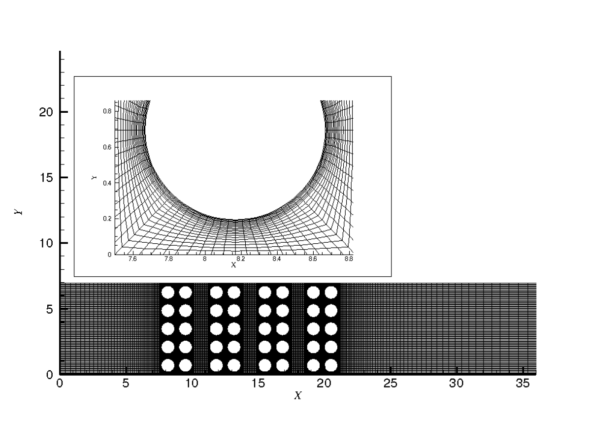
Figure 3: A side view of computational mesh used for the LES with a close look-up around a cylinder.

Figure 3 shows a side view of the computational grid with a close look-up around a cylinder. The total number of grid elements used for the present simulation is around $3.4$ million. The mesh has an embedded region of fine mesh designed for each cylinder in order to enhance the mesh resolution near the cylinder without incurring too large an increase in the total number of mesh elements. The first cell adjacent to the cylinder is within the range $\Delta y^{+}<11.8$ in wall units, which satisfies the requirements of the Wener-Wengle wall-layer model used for wall-modelling LES. Prior to the present simulation, with the standard Smagorinsky subgrid scale model, a simulation based coarse grid resolution were carried out to determine the resolution.

With fully developed turbulent flows, periodic boundary conditions are justified to use along the normal ($y$) and spanwise ($z$) direction. For the inlet boundary condition, a simple uniform velocity profile is assumed and the turbulent intensity set to zero. Hence, the turbulence fluctuations at the inlet was not accounted for temporally and spatially. Nevertheless, a length $7.5D$ before the first column bank is used to allow the development of turbulence. At the exit boundary, the solution variables from the adjacent interior cells are extrapolated to satisfy the mass conservation.

The simulation is advanced with non-dimensional time step $\Delta tU_{o}/D\approx 1.4\times 10^{-3}$ that yields maximum Courant-Friedrichs-Lewy (CFL) number 0.7. For the carrier phase, the first-order statistics are collected by integrating the governing equations over an interval of $25D/U_{o}$, and all the statistics are averaged over the $40$ sampling points across in the spanwise direction.

2.4 Calculation of particle trajectories

A parallel Lagrangian particle tracking module was developed to calculate trajectories of heavy particles in flow fields resolved by LES. The particle localization algorithm on unstructured grids proposed by Haselbacher et al.[29] was used to locate the cell which contains the current particle position. In this study, the focus is on the deposition of non-inter-collision, rigid, spherical and heavy particles on in-line tube-banks by impact; the concentration of particles is dilute enough to make one-way coupling assumption. The momentum balance equation of particles discussed by Maxey and Riley[30] is simplified in this work with taking into account the drag force merely. We thus can write the particle equation of motion involving the non-linear form of the drag law with the point particle approximation

$$\frac{\mathrm{d}\mathbf{u}_{p}}{\mathrm{d}t}=\frac{1}{\tau_{p}}C_{D}\frac{Re_{p}}{24}(\mathbf{u}-\mathbf{u}_{p}),$$ (26)

where $\mathbf{u_{p}}$ is the particle velocity and $\mathbf{u}$ the instantaneous fluid velocity at the particle location, $\tau_{p}$ is the particle response time. An empirical relation for $C_{D}$ from Morsi and Alexander[31], which is applicable to a wide range of particle Reynolds number with sufficiently high accuracy, is employed.

$$C_{D}=c_{1}+\frac{c_{2}}{Re_{p}}+\frac{c_{3}}{Re_{p}^{2}},$$ (27)

in which $c_{1},c_{2},c_{3}$ are constants. The above empirical expression exhibits the correct asymptotic behavior at low as well as high values of $Re_{p}$.

The position $\mathbf{x}_{p}$ of particles is obtained from the kinematic relationship

$$\frac{\mathrm{d}\mathbf{x}_{p}}{\mathrm{d}t}=\mathbf{u}_{p}$$ (28)

The boundary condition for the above equation is that the particle is captured by the wall when its center away the nearest wall surface is less than its radius. This is not properly treated in the default discrete phase model (DPM) provided by ANSYS FLUENT. Furthermore, this error has a significant effect upon predictions concerning the deposition of heavy particles under investigation.

From a statistically stationary LES flow field, equation: (28) is started to be integrated in time using the second-order Adams-Bashforth scheme to get particle trajectories, whilst equation: (26) is integrated with the second-order accurate Gear2 (backward differentiation formulae) scheme that is applicable to stiff systems. Since it is only by chance that a particle coincides with the cell centroid, at which the fluid solution is stored as part of the computation of the underlying flow field with the unstructured-grid based collocated cell centroid storage finite volume method, a quadratic scheme based on least-squares velocity gradient reconstruction is used to interpolate the fluid velocity to the particle location without consideration of the effect of sub-grid scale. For the second-order accurate carrier phase solver, the quadratic scheme is found to be sufficient to accurately resolve the particle motions.

Results on for three sets of particles ($St=0.35,0.086,0.0075$) are obtained by following the trajectories of $10^{7}$ particles which are continuously released into the computational domain. This large number of particles trajectories are crucial in order to present statistically significant results on the particles phase which interacts with the vortex dynamics in spatial and temporal domain. However, the unsteady deposition issue of particles on the tube-banks has not been taken into account, which results in a significant simplification on the interaction of incoming particles with deposition particles.

2.5 A particle-wall collision model

Particle-wall collisions play an important role in particle-laden two-phase flows because it effects the deposition, accumulation on wall surfaces. In this work, the aim is not to seek a new particle-wall-collision model, instead a well-known dry particle-wall-collision model from Thornton and Ning[32] was implemented to account for the energy loss resulting from the particle-wall-collision. The energy loss resulting from impact upon a wall is normally characterized by the coefficient of restitution (CoR) $e$ that is defined by

$$e=\frac{v_{r}^{n}}{v_{i}^{n}}$$ (29)

where $v_{r}^{n}$ is the rebound normal velocity and $v_{i}^{n}$ the incident normal velocity. Then, the loss of kinetic energy $\Delta E$ of a particle with mass $m_{p}$ is given by

$$\Delta E=\frac{1}{2}m_{p}\left({v_{i}^{n}}^{2}-{v_{r}^{n}}^{2}\right)=\frac{1}{2}m_{p}{v_{i}^{n}}^{2}\,\left(1-e^{2}\right).$$ (30)

In the case of elastic impact, $e=1$ due to no energy loss occurred. When $e=0$, the maximum incident normal velocity is normally referred to as the critical sticking velocity $v_{s}$. Then from

$$\Delta E=\frac{1}{2}m_{p}v_{s}^{2},$$ (31)

$e$ is given by

$$e=\left[1-\left(\frac{v_{s}}{v_{i}^{n}}\right)^{2}\right].$$ (32)

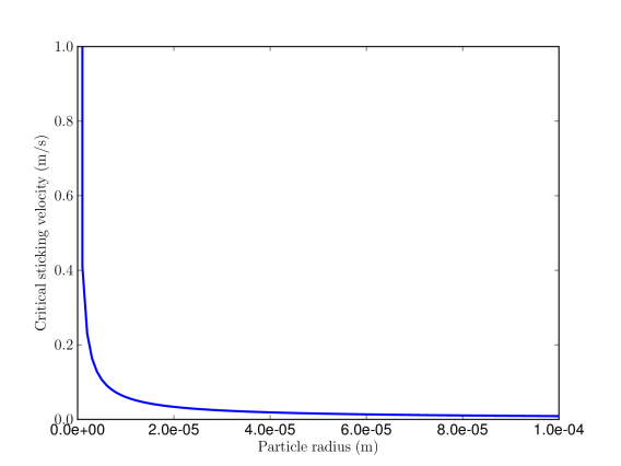
Figure 4: Critical sticking velocity as a function of particle radius.

If $v_{i}^{n}$ is higher than $v_{s}$ then $e>0$ and the particle can bounce off the wall upon impact; if not, the particle sticks the wall and $e=0$. The critical sticking velocity $v_{s}$ is normally determined by the properties of the particle and wall. Figure 4 shows the variation of critical sticking velocity for a wide range of particle radii. It can be observed that the smaller the particle radius is, the larger the critical sticking velocity is. Therefore, it is easier for larger particles get bounce upon impact. Figure 5 illustrates how the coefficient of restitution with the particle incident normal velocity. When the particle incident normal velocity is approaching $0.2~{}\mathrm{m/s}$ the coefficient of restitution is close to $0.985$.

In this study, the critical sticking velocities for three sets of particles considered are calculated and input as parameters before starting particle tracking. Therefore, this model can be used to determine whether a particle sticks to or rebound from a wall upon impact with the wall.

3 Results and discussions

3.1 Results on the carrier phase

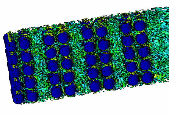
Figure 6: Instantaneous velocity magnitude based on the normalized Q criterion equalling to $0.08$.

Figure 6 shows the contour of the instantaneous velocity magnitude based on the normalized Q criterion equalling to 0.08. The top cylinder in the first column develops a laminar boundary layer and has some kind of laminar vortex shedding. However, this was not observed from the downstream cylinders. Large coherent structures are visible in the gaps between tube-banks, but they are not as well organized and periodic as in typical Karman vortex streets for a single cylinder at the similar Reynolds number. Large coherent structures between two adjacent column cylinders in the same pair are not as obvious as those in the gaps. This may result from the relatively small gap in every pair destroys the development of the wake. Finally, the flow is evolving into a turbulent flow like a grid turbulence from the final pair of tube-banks.

Following Shim et al.[33], the coefficient for the mean pressure distribution on the cylinder surface is define as

$$\overline{C}_{p}=\frac{\left<p\right>_{T}-p_{ref}}{q_{ref}},$$ (33)

where $\left<p\right>_{T}$ denotes an ensemble average across the spanwise direction for all the sampling points on the cylinder surface over the sampling time interval $T$, and

$$q_{ref}=\frac{1}{2}\rho u_{g}^{2}.$$ (34)

In order to make $\overline{C}_{p}$ equal to unit at the front stagnation point for every cylinder, the corresponding static pressure $p_{ref}$ is calculated according to equation 33, $\overline{C}_{p}$ is hence determined around the cylinder surface.

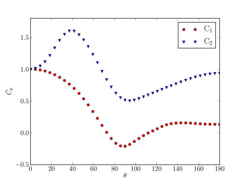
(a)

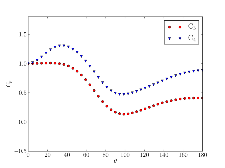
(b)

Figure 7: Mean pressure distribution on the middle cylinder surface. Definition of $\overline{C}_{p}$ based on [33]. (a) the first pair tube banks, (b) the second pair tube banks.

Comparisons of $\overline{C}_{p}$ on the middle cylinders surface from the first and second pair of tube-banks are shown in figure 7. It can be observed that $\overline{C}_{p}$ is of the standard shape, which $\overline{C}_{p}$ normally develops on a single circular cylinder. However, $\overline{C}_{p}$ on the second cylinder is of a $\mathbf{S}$ shape, indicating there is a region in the front side of the cylinder that has higher pressure than the front stagnation point. This higher pressure distribution results from the impingement of the wake from the preceding cylinder on the front side. The phenomena was also observed in the experimental measurements for a tube-banks with a close longitudinal pitch from Shim et al. [33]. From 7b, It can be observed that $\overline{C}_{p}$ on $C_{3}$ is also of the standard shape for a single cylinder, but it has a relatively high base pressure. $\overline{C}_{p}$ on the following cylinder $C_{3}$ has the similar shape like to the one on $C_{4}$, implying that the shedding vortex from $C_{3}$ impacts on the front side of $C_{4}$.

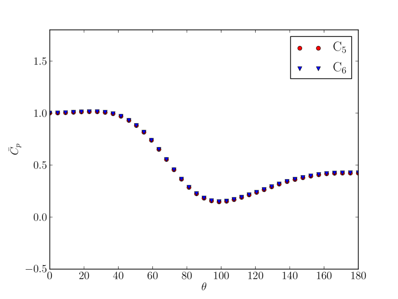
(a)

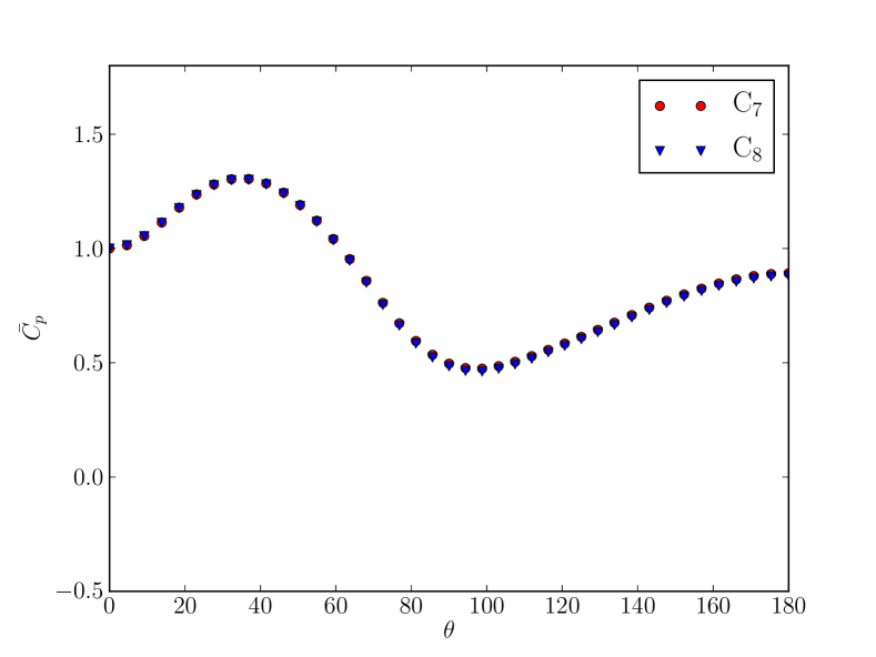
(b)

Figure 8: Mean pressure distribution on the middle cylinder surface. Definition of $\overline{C}_{p}$ based on [33]. (a) the third pair tube banks, (b) the fourth pair tube banks.

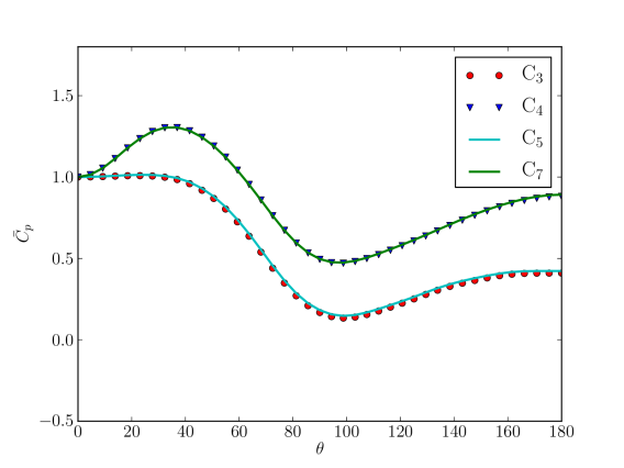
Figure 9: Comparison of mean pressure distribution on the middle cylinder surface from the second, third and fourth pair of tube-banks

Figure 8 shows $\overline{C}_{p}$ on the middle cylinders from the third and fourth pair of tube-banks. Interestingly, there is no discernible discrepancy between the two cylinders in the same pair. For the cylinder $C_{5},C_{6}$, $\overline{C}_{p}$ behaviors like a single cylinder. Similar results on $\overline{C}_{p}$ are observed for the cylinder $C_{7},C_{8}$, but they are higher than unit in the front side of cylinders. This is further confirmed by the figure 9 which shows no discrepancy between the $\overline{C}_{p}$ on cylinders from different pairs. This implies that the shedding vortex from the third pair of tube-banks impinges on the final pair of tube banks. This impingement may result in different surface pressure distributions on cylinder $C_{7},C_{8}$, but after the scaling based on the equation: 33 $\overline{C}_{p}$ displays no significant difference.

3.2 Results on the particle phase

3.2.1 Sample particle trajectories and bounce upon impact

Figure 10 shows some sample particle trajectories across the tube-banks. With the present particle-wall collision model, it can be clearly observed that some particles rebound upon impact on the cylinders. This normally results in a smaller rebounce velocity even particles peel on the surface of cylinders as a result of energy loss.

3.2.2 Deposition efficiency on tube-banks

The deposition efficiency for a single cylinder(or known as collection efficient) is normally defined as

$$\eta_{sc}=\frac{N_{dep}}{N_{tot}},$$ (35)

where $N_{dep}$ is the number of deposition particles on the cylinder, and $N_{tot}$ is the number of uniformly distributed particles in the upstream cross-sectional area of the cylinders.

Nevertheless, in the present case that particles deposit on in-line tube-banks, overall deposition efficiencies for each pair of tube-banks have to be defined differently. The deposition efficiency for the first pair is determined by taking the number of particles in the upstream cross-sectional area of the first column cylinders and comparing that number to the number of particles actually deposited on the first pair of tube-banks. This reads

$$\eta_{pair1}=\frac{N_{pair1}}{\frac{5}{6.94}N_{tot}},$$ (36)

where $N_{pair1}$ is the number of deposition particles on the first pair of tube-banks, $N_{tot}$ is the total number released from the upstream, $5/6.94$ is ratio of the cross-sectional area of the first column cylinders to the cross-sectional area of the computational domain. However, since it is difficult to define how many particles are in the upstream cross-sectional area of the succeeding tube-banks, the number is assumed to be simply the number in the particle release plane cross-sectional area $5N_{tot}/6.94$ minus the number of particles deposited on the preceding tube-banks. For example, the deposition efficiency of the fourth pair of tube-banks can be written as

$$\eta_{pair_{4}}=\frac{N_{pair_{4}}}{\Big{(}\frac{5}{6.94}N_{tot}-\sum_{i=1}^{3}N_{{pair_{i}}}\Big{)}}.$$ (37)

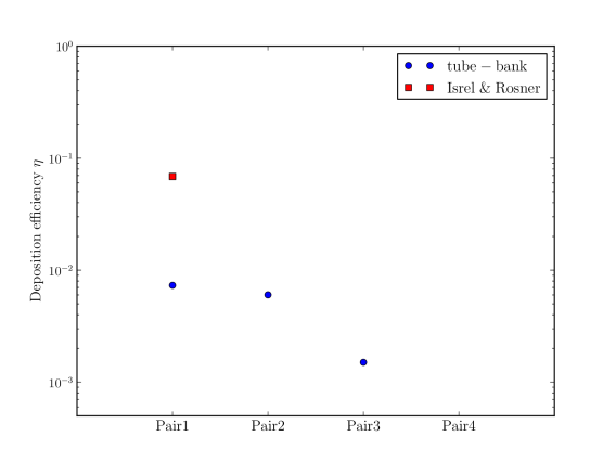
Figure 11: Deposition efficiency of particles $St=0.35$ across tube-banks and a comparison against to the results on a single cylinder from [7]

The computed results on deposition efficiency across the tube-banks are shown in figure 11, 12 and 13.

Figure 11 also includes a result on deposition efficiency on a single cylinder based on the curve fit proposed by Israel and Rosner[7]. The particle $St=0.35$ an effective Stokes number $St_{eff}$ equalling to $0.21$ based on equation  2, which is in the valid range of above curve-fit. First, it can be seen that the deposition efficiency for $St=0.35$ is falling along the flow direction. Second, the deposition efficiency for the first pair of tube-banks is significantly lower than that of a single circular cylinder. This may result from the fact that flow channeling is occurring between two vertically adjacent cylinders. However, it can be observed that there is a considerable increase of the deposition efficiency for particles $St=0.086,0.0075$, which is not consistent with theoretical results on a single cylinder. A possible explanation is that a large amount of particles are entrained into the wake of the back-banks of each pair of tube-banks and get deposition by back-side impaction (see [8]).

3.2.3 Deposition fraction across the tube-banks

Deposition data of three sets of particles ($St=0.35,0.086,0.0075$) on tube-banks are presented here. The pair of tube-banks shown in figure 2 are designated by $\mathrm{pair1}$ (upstream) through $\mathrm{pair4}$ (downstream); the upstream and downstream column of tube-banks in each pair are designated by front bank and back bank. $10^{7}$ particles are released into the computational continuously for an interval of $1000$ continuous time steps, in order to both collect enough particles and account for the unsteady effect.

Figure 14, 15 and 16 show that the variations of fraction of total deposition particles across the whole tube-banks for the three sets particles. As can be seen, for the particle $St=0.35$, across the four pairs of the tube-banks the fraction of deposition particles on the pair1 is significantly higher than on the downstream pair of tube-banks, pair2, pair3 and pair4. On the other hand, the fraction of deposition on the front bank in the same pair of tube-banks is higher than on the back bank, especially for the pair1. This may result from the fact that a significant part of this set of particle is entrained in the bulk flow between cylinders and don’t follow the shedding vortex from the preceding cylinders (see figure 10). However, the computed results for particles $St=0.086,0.0075$ are not consistent with those results for $St=0.345$. Although the fraction of deposition on the pair3 and pair4 are lower than the preceding two pairs, a striking difference is noted when compared to the particle $St=0.35$.

It can be observed from figure 17a that the back-side deposition on the back banks of pair1 and pair2, for particles $St=0.0075$ result in considerably higher fraction of deposition. For the back-side deposition, Haugen et al.[8] argued that when particle with response time $\tau_{p}$ is close to the eddy time $\tau_{eddy}$, they normally follow the eddies in the wake of the tube-banks and gain enough momentum to impact on the cylinders.

4 Concluding remarks

A large eddy simulation of inertia deposition, impact of heavy particles on an in-line tube-banks in a turbulent flow are performed. The flow Reynolds number, based on the cylinder diameter $D$ and flow velocity between the gap of two vertically adjacent cylinders, is $33960$. Flow structures across the tube bank based on the normalized Q criterion is presented. Following the formula for mean pressure distribution for cylinders in tube-banks proposed by Shim et al.[33], mean pressure distribution on the middle cylinder from each tube-bank is present. The $S$ shape of mean pressure distribution is observed on the back-bank of the first pair and second pair of tube-banks. Further, the mean pressure distribution on the each tube-bank within the third pair of tube-banks displays almost exactly the same behavior. Similar behavior is observed on the final pair of tube-banks.

The results for three sets of particles ($St=0.35,0.086,0.0075$) are based on $10^{7}$ particles tracked through Lagrangian point particle tracking approach. The particle bounce upon impact is taken into account through a particle-wall collision model. Some sample particle trajectories across tube-banks are shown, which shows that some particles rebound from the cylinder surface upon impact. The deposition efficiency for the three sets of particles are presented across the tube-banks. Moreover, the fraction deposition of particles across each tube-banks are provided. It is observed that for the particle $St=0.35$ most of particles get deposition on the first tube-banks, especially on the first column. This is consistent with practical experience that the first column of tube-banks plays a protection role on mitigating fouling on the succeeding tube-banks. Based on the effective Stokes number proposed by Israel and Rosner[7], the overall deposition efficiency of the particle $St=0.35$ on the first pair of tube-banks is significantly lower than that of a single circular cylinder. Nevertheless, the results on deposition efficiency for particles $St=0.086,0.0075$ are not consistent with those of particles $St=0.35$. A display of deposition particle on tube-banks suggests that much more of smaller particles get deposition on the back-side of the back-banks. This may due to the fact that the smaller particles are easier to be entrained into the wake and impact onto the back-side of cylinders. This issue needs further investigations.

5 acknowledgments

We wish to acknowledge the support of British Energy (Part of EDF).

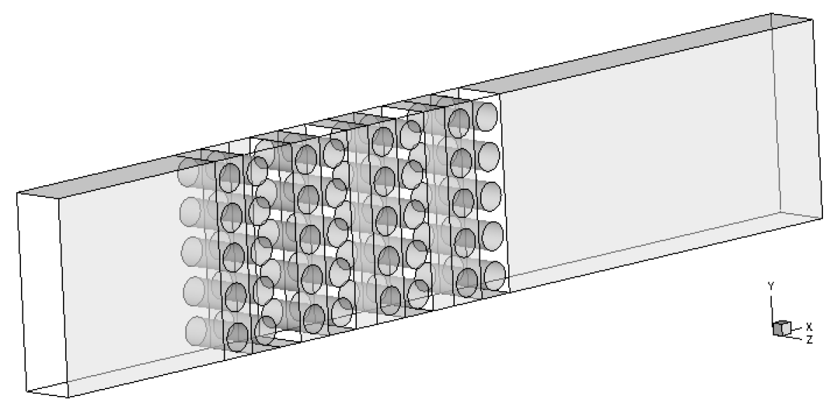
Figure 2: Configuration of four by five pairs of in-line tube banks.

Figure 5: Coefficient of restitution $e$ as a function of particle incident normal velocity.

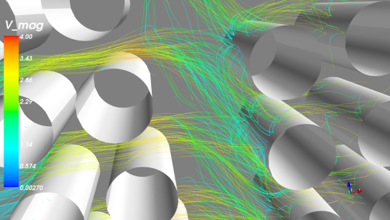
Figure 10: Sample particle trajectories and bounce upon impact on cylinders for particles $St=0.35$

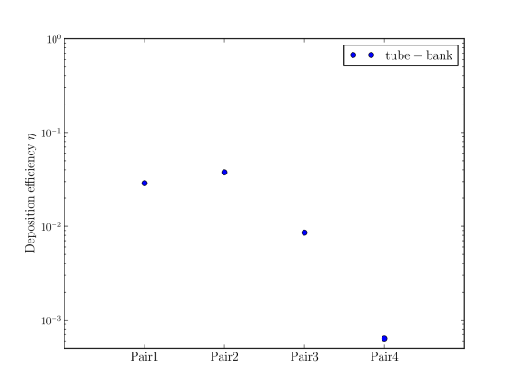
Figure 12: Deposition efficiency of particles $St=0.086$ across tube-banks

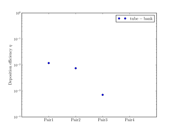
Figure 13: Deposition efficiency of particles $St=0.0075$ across tube-banks

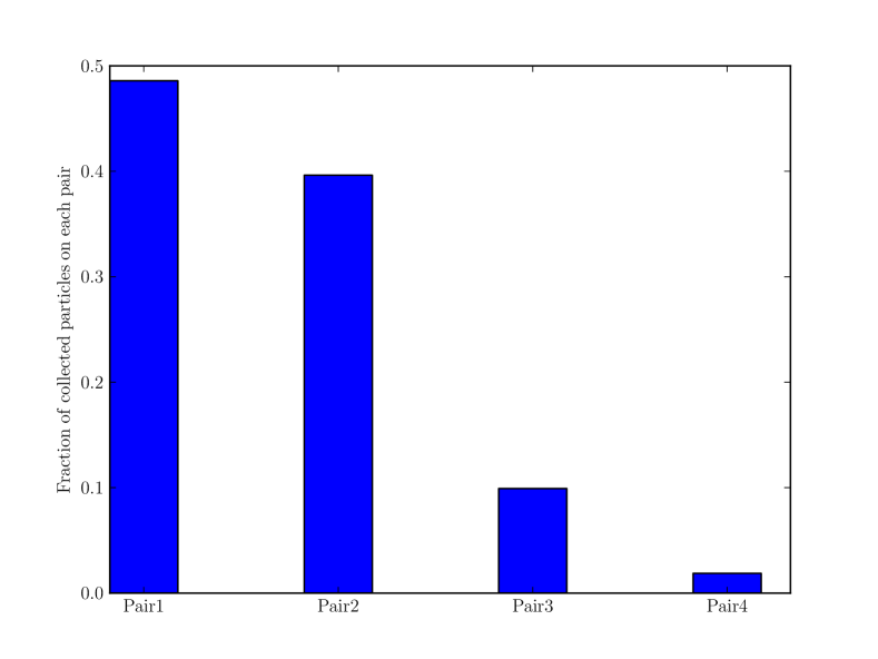
(a)

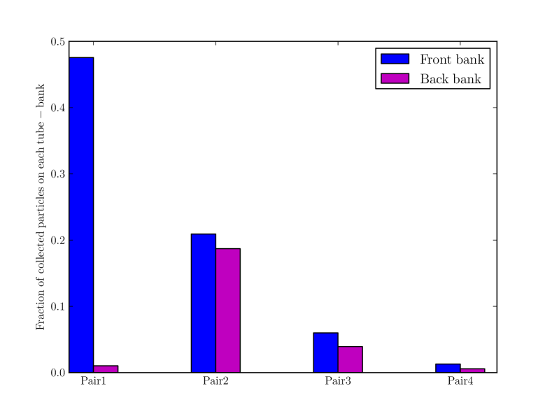
(b)

Figure 14: Fraction of total deposition particles across tube-banks for particles $St=0.35$ (a) each pair of tube-banks, (b) each tube-banks.

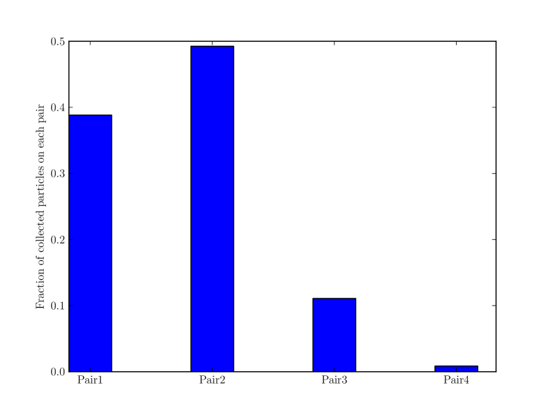
(a)

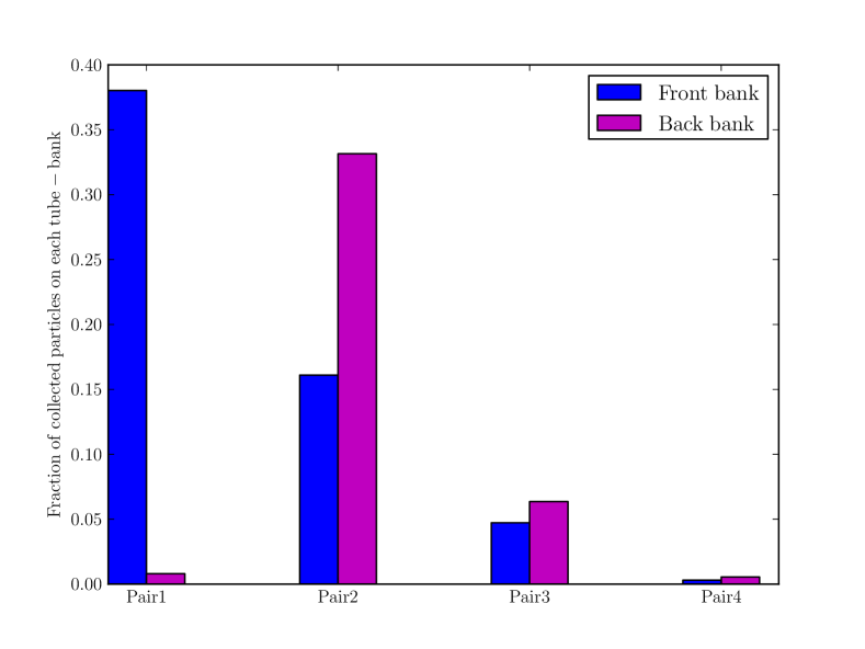
(b)

Figure 15: Fraction of total deposition particles across tube-banks for particles $St=0.086$ (a) each pair of tube-banks, (b) each tube-banks.

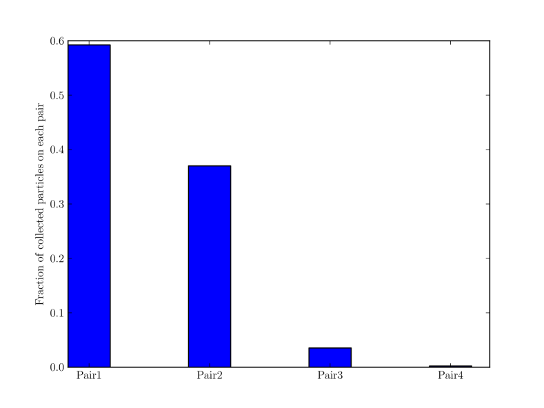
(a)

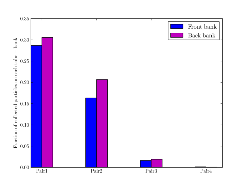
(b)

Figure 16: Fraction of total deposition particles across tube-banks for particles $St=0.0075$ (a) each pair of tube-banks, (b) each tube-banks.

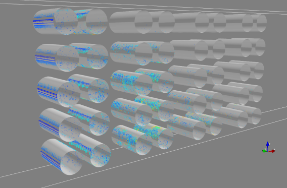
(a)

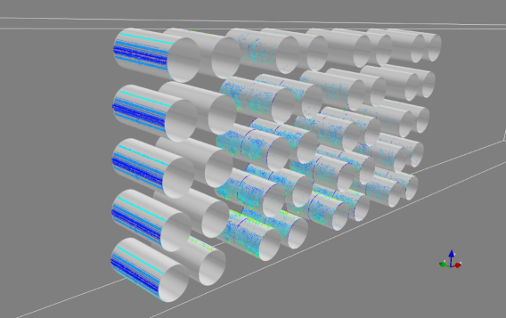
(b)

Figure 17: Deposition particles on tube-banks (a) $St=0.0075$, (b) $St=0.35$.

References

- Friedlander and Johnstone [1957] S. K. Friedlander, H. F. Johnstone, Deposition of suspended particles from turbulent gas streams, Industrial & Engineering Chemistry 49 (1957) 1151–1156.
- Reeks [1983] M. W. Reeks, The transport of discrete particles in inhomogeneous turbulence, Journal of Aerosol Science 14 (1983) 729–739.
- Kallio and Reeks [1989] G. A. Kallio, M. W. Reeks, A numerical simulation of particle deposition in turbulent boundary layers, International Journal of Multiphase Flow 15 (1989) 433–446.
- Helgesen and Matteson [1991] J. K. Helgesen, M. J. Matteson, Particle mixing and diffusion in the turbulent wake of cylinder arrays, Experiments in Fluids 10 (1991) 333–340.
- Helgesen and Matteson [1994] J. K. Helgesen, M. J. Matteson, Particle mixing and diffusion in the turbulent wake of a single cylinder, Aerosol Science and Technology 20 (1994) 111–126.
- Brun et al. [1955] R. J. Brun, W. Lewis, P. J. Perkins, J. S. Serafini, Impingement of cloud droplets on a cylinder and procedure for measuring liquid-water content and droplet sizes in supercooled clouds by rotating multicylinder method (1955).
- Israel and Rosner [1982] R. Israel, D. E. Rosner, Use of a generalized stokes number to determine the aerodynamic capture efficiency of non-stokesian particles from a compressible gas flow, Aerosol Science and Technology 2 (1982) 45–51.
- Haugen et al. [2010] N. E. L. Haugen, S. Kragset, M. Bugge, R. Warnecke, M. Weghaus, Particle impaction efficiency and size distribution in a mswi super heater tube bundle, Arxiv preprint arXiv:1008.5040 (2010).
- Jun and Tabakoff [1994] Y. D. Jun, W. Tabakoff, Numerical simulation of a dilute particulate flow (laminar) over tube banks, Journal of Fluids Engineering 116 (1994) 770–777.
- Bouris et al. [2001] D. Bouris, G. Papadakis, G. Bergeles, Numerical evaluation of alternate tube configurations for particle deposition rate reduction in heat exchanger tube bundles, International Journal of Heat and Fluid Flow 22 (2001) 525–536.
- Tian et al. [2007] Z. F. Tian, J. Y. Tu, G. H. Yeoh, Numerical modelling and validation of gas-particle flow in an in-line tube bank, Computers & chemical engineering 31 (2007) 1064–1072.
- Dehbi [2008] A. Dehbi, Turbulent particle dispersion in arbitrary wall-bounded geometries: A coupled CFD-Langevin-equation based approach, International Journal of Multiphase Flow 34 (2008) 819–828.
- Jin et al. [2015] C. Jin, I. Potts, M. Reeks, A simple stochastic quadrant model for the transport and deposition of particles in turbulent boundary layers, Physics of Fluids (1994-present) 27 (2015) 053305.
- Dehbi and Martin [2011] A. Dehbi, S. Martin, Cfd simulation of particle deposition on an array of spheres using an euler/lagrange approach, Nuclear Engineering and Design (2011).
- Williamson [1996] C. H. K. Williamson, Vortex dynamics in the cylinder wake, Annual Review of Fluid Mechanics 28 (1996) 477–539.
- Benhamadouche and Laurence [2003] S. Benhamadouche, D. Laurence, LES, coarse LES, and transient RANS comparisons on the flow across a tube bundle, International Journal of Heat and Fluid Flow 24 (2003) 470–479.
- Jin et al. [2016] C. Jin, I. Potts, D. Swailes, M. Reeks, An LES study of turbulent flow over in-line tube-banks and comparison with experimental measurements, arXiv preprint arXiv:1605.08458 (2016).
- Apte et al. [2003] S. V. Apte, K. Mahesh, P. Moin, J. C. Oefelein, Large-eddy simulation of swirling particle-laden flows in a coaxial-jet combustor, International Journal of Multiphase Flow 29 (2003) 1311–1331.
- Riber et al. [2009] E. Riber, V. Moureau, G. M., T. Poinsot, O. Simonin, Evaluation of numerical strategies for large eddy simulation of particulate two-phase recirculating flows, Journal of Computational Physics 228 (2009) 539–564.
- Leonard [1974] A. Leonard, Energy cascade in large-eddy simulations of turbulent fluid flows, Adv. Geophys 18 (1974) 237–248.
- Smagorinsky [1963] J. Smagorinsky, General circulation experiments with the primitive equations, Monthly weather review 91 (1963) 99–164.
- Lilly [1966] D. K. Lilly, On the application of the eddy viscosity concept in the inertial sub-range of turbulence, National Center for Atmospheric Research, 1966.
- Deardorff [1970] J. W. Deardorff, A numerical study of three-dimensional turbulent channel flow at large reynolds numbers, Journal of Fluid Mechanics 41 (1970) 453–480.
- Piomelli et al. [1988] U. Piomelli, P. Moin, J. H. Ferziger, Model consistency in large eddy simulation of turbulent channel flows, Physics of Fluids 31 (1988) 1884.
- Germano et al. [1991] M. Germano, U. Piomelli, P. Moin, W. H. Cabot, A dynamic subgrid-scale eddy viscosity model, Physics of Fluids A: Fluid Dynamics 3 (1991) 1760.
- Lilly [1992] D. K. Lilly, A proposed modification of the germano subgrid-scale closure method, Physics of Fluids A: Fluid Dynamics 4 (1992) 633.
- Werner et al. [1993] H. Werner, H. Wengle, et al., Large-eddy simulation of turbulent flow over and around a cube in a plate channel, Turbulent Shear Flows 8 (1993) 155–168.
- Hall [1994] D. Hall, The transport of particles through CAGR boilers, 1994.
- Haselbacher et al. [2007] A. Haselbacher, F. M. Najjar, J. P. Ferry, An efficient and robust particle-localization algorithm for unstructured grids, Journal of Computational Physics 225 (2007) 2198–2213.
- Maxey and Riley [1983] M. R. Maxey, J. J. Riley, Equation of motion for a small rigid sphere in a nonuniform flow, Physics of Fluids 26 (1983) 883.
- Morsi and Alexander [1972] S. A. Morsi, A. J. Alexander, An investigation of particle trajectories in two-phase flow systems, Journal of Fluid Mechanics 55 (1972) 193–208.
- Thornton and Ning [1998] C. Thornton, Z. Ning, A theoretical model for the stick/bounce behaviour of adhesive, elastic-plastic spheres, Powder technology 99 (1998) 154–162.
- Shim et al. [1988] K. C. Shim, R. S. Hill, R. I. Lewis, Fluctuating lift forces and pressure distributions due to vortex shedding in tube banks, International Journal of Heat and Fluid Flow 9 (1988) 131–146.