The evolution to localized and front solutions in a non-Lipschitz reaction-diffusion Cauchy problem with trivial initial data

Abstract

In this paper, we establish the existence of spatially inhomogeneous classical self-similar solutions to a non-Lipschitz semi-linear parabolic Cauchy problem with trivial initial data. Specifically we consider bounded solutions to an associated two-dimensional non-Lipschitz non-autonomous dynamical system, for which, we establish the existence of a two-parameter family of homoclinic connections on the origin, and a heteroclinic connection between two equilibrium points. Additionally, we obtain bounds and estimates on the rate of convergence of the homoclinic connections to the origin.

1 Introduction

In this paper, we study classical bounded solutions $u:\mathbb{R}\times[0,T]\to\mathbb{R}$ to the non-Lipschitz semi-linear parabolic Cauchy problem

$$u_{t}-u_{xx}=u|u|^{p-1}\ \ \ \text{ on }\mathbb{R}\times(0,T],$$ (1)

$$u=0\ \ \ \text{ on }\mathbb{R}\times\{0\},$$ (2)

with $0<p<1$ and $T>0$ (which we henceforth refer to as [CP]). The primary achievement of the paper is the establishment of the existence of a two-parameter family of localized spatially inhomogeneous solutions to [CP] for which $u(x,t)\to 0$ as $|x|\to\infty$ uniformly for $t\in[0,T]$; the secondary achievement of the paper is the establishment of front solutions to [CP], which approach $\pm(1-p)^{1/(1-p)}t$ as $|x|\to\pm\infty$ uniformly for $t\in[0,T]$. We note here that for $p\geq 1$ in (1), then the unique bounded classical solution with initial data (2) is the trivial solution, see for example [15, Theorem 4.5].

Qualitative properties of non-negative (non-positive) solutions to (1) when $0<p<1$, with non-negative (non-positive) initial data, and for which $u(x,t)$ is bounded as $|x|\to\infty$ uniformly for $t\in[0,T]$, have been determined in [1], [12], [20], [14] and [16]. However, we note that any non-negative (non-positive) classical bounded solution to [CP] must be spatially homogeneous for $t\in[0,T]$, see for example [1, Corollary 2.6]. Thus, the solutions constructed in this paper are two signed on $\mathbb{R}\times[0,T]$. The authors are currently unaware of any studies of two signed solutions to (1)-(2) with $0<p<1$. Generic local results for spatial homogeneity of solutions to semi-linear parabolic Cauchy problems with homogeneous initial data depend upon uniqueness results, see for example, [16]. For results concerning the related problem of asymptotic homogeneity (in general, asymptotic symmetry) as $t\to\infty$ of non-negative (non-positive) global solutions to semi-linear parabolic Cauchy problems, we refer the reader to the survey article [22].

Non-negative (non-positive), spatially inhomogeneous solutions to (1) for $p>1$ have been considered in [10], [26] [27], [21], [9], [11], [24], [8], [5] and [25] with the focus primarily on critical exponents for finite time blow-up of solutions, and conditions for the existence of global solutions (see the review articles [13] and [7]). Moreover, for $p>1$, solutions to (1) with two signed initial data have been considered in [18] and [19], whilst boundary value problems have been studied in [3] and [4].

The paper is structured as follows; in Section 2 we introduce the self-similar solution structure for [CP], and hence, determine an ordinary differential equation related to (1); the remainder of the paper concerns the study of particular solutions to this ordinary differential equation, which is re-written as an equivalent two-dimensional non-autonomous dynamical system. Specifically, in Section 3 we establish the existence of a two-parameter family of homoclinic connections on the equilibrium $(0,0)$. Additionally, we determine bounds and estimates on the asymptotic approach of these solutions to $(0,0)$. In Section 4, we establish the existence of a heteroclinic connection between the equilibrium points $(\pm(1-p)^{1/(1-p)},0)$.

2 Self-Similar Structure

With $0<p<1$ and $T>0$, we refer to $u:\mathbb{R}\times[0,T]\to\mathbb{R}$ as a solution to [CP] when $u$ satisfies (1)-(2) with regularity,

$$u\in L^{\infty}(\mathbb{R}\times[0,T])\cap C(\mathbb{R}\times[0,T])\cap C^{2,1}(\mathbb{R}\times(0,T]).$$ (3)

Observe that $u^{\pm}:\mathbb{R}\times[0,T]\to\mathbb{R}$ given by

$$u^{\pm}(x,t)=\pm((1-p)t)^{1/(1-p)}\ \ \ \forall(x,t)\in\mathbb{R}\times[0,T]$$

are the maximal and minimal solutions to [CP] (see [15, Chapter 8]), and hence any solution $u:\mathbb{R}\times[0,T]\to\mathbb{R}$ to [CP] must satisfy,

$$u^{-}(x,t)\leq u(x,t)\leq u^{+}(x,t)\ \ \ \forall(x,t)\in\mathbb{R}\times[0,T].$$ (4)

To construct spatially inhomogeneous solutions to [CP], we consider, for any fixed $x_{0}\in\mathbb{R}$, self-similar solutions $u:\mathbb{R}\times[0,T]\to\mathbb{R}$ of the form,

$$u(x,t)=\begin{cases}w\left(\frac{x-x_{0}}{t^{1/2}}\right)t^{1/(1-p)}&,(x,t)\in\mathbb{R}\times(0,T],\\ 0&,(x,t)\in\mathbb{R}\times\{0\},\end{cases}$$ (5)

with $w:\mathbb{R}\to\mathbb{R}$ to be determined. Now, $u:\mathbb{R}\times[0,T]\to\mathbb{R}$ given by (5) is a solution to [CP] if and only if there exist constants $\alpha$, $\beta\in\mathbb{R}$ such that $w:\mathbb{R}\to\mathbb{R}$ satisfies the following zero-value problem, namely,

$$w^{\prime\prime}+\frac{1}{2}\eta w^{\prime}+w|w|^{p-1}-\frac{1}{(1-p)}w=0\ \ \ \forall\eta\in\mathbb{R},$$ (6)

$$w(0)=\alpha,\ \ \ w^{\prime}(0)=\beta,$$ (7)

$$w\in C^{2}(\mathbb{R})\cap L^{\infty}(\mathbb{R}).$$ (8)

Here $\eta=(x-x_{0})/t^{1/2}$, and we observe that the ordinary differential equation (6) is both non-autonomous and non-Lipschitz. It is convenient to introduce

$$x=w,\ \ \ y=w^{\prime},$$

after which the problem (6)-(8) is equivalent to the zero-value problem for the two-dimensional, non-Lipschitz, non-autonomous, dynamical system,

$$x^{\prime}=y$$ (9)

$$y^{\prime}=\frac{1}{(1-p)}x-x|x|^{p-1}-\frac{1}{2}\eta y\ \ \ \forall\eta\in\mathbb{R},$$ (10)

$$(x(0),y(0))=(\alpha,\beta),$$ (11)

$$(x,y)\in C^{1}(\mathbb{R})\cap L^{\infty}(\mathbb{R}).$$ (12)

We refer to the equivalent zero-value problems in (6)-(8) and (9)-(12) as (S). Our objective is now to investigate those $(\alpha,\beta)\in\mathbb{R}^{2}$ for which (S) has a non-trivial solution. It is instructive to note, at this stage, via (4), that we may conclude that any solution to (S) must satisfy the inequality,

$$-(1-p)^{\frac{1}{(1-p)}}\leq w(\eta)\leq(1-p)^{\frac{1}{(1-p)}}\ \ \ \forall\eta\in\mathbb{R},$$ (13)

whilst, following [1, Corollary 2.6], any non-constant solution to (S) must be two-signed in $w$.

3 Homoclinic Connections

In this section we establish the existence of a two parameter family of homoclinic connections for (S) on the equilibrium point $(0,0)$ of the dynamical system (9)-(10), and establish decay rates to the equilibrium point $(0,0)$ as $|\eta|\to\infty$ on these homoclinic connections.

3.1 Existence

In this subsection, we establish the existence of homoclinic connections attached to the equilibrium point $(x,y)=(0,0)$ of the dynamical system (9)-(10). To begin, observe that ${\bf{Q}}:\mathbb{R}^{3}\to\mathbb{R}^{2}$, where

$${\bf{Q}}(x,y,\eta)=(Q_{1},Q_{2})(x,y,\eta)=\left(y,\frac{1}{(1-p)}x-x|x|^{p-1}-\frac{1}{2}\eta y\right)\ \ \ \forall(x,y,\eta)\in\mathbb{R}^{3}$$ (14)

is such that ${\bf{Q}}\in C(\mathbb{R}^{3})$, but also that ${\bf{Q}}$ is not locally Lipschitz continuous on $\mathbb{R}^{3}$ (note that ${\bf{Q}}$ is locally Lipschitz continuous on $\mathbb{R}^{3}\backslash N$, with $N$ any neighbourhood of the plane $x=0$). We now have,

Theorem 1.

The problem (S) with zero-value $(\alpha,\beta)\in\mathbb{R}^{2}$ has a solution for $\eta\in[-\delta,\delta]$ (not necessarily unique), where $\delta=1/(1+M)$ and

$$M=\max_{(x,y,\eta)\in R}|{\bf{Q}}(x,y,\eta)|$$

with

$$R=\{(x,y,\eta)\in\mathbb{R}^{3}:|x-\alpha|\leq 1,\ |y-\beta|\leq 1,\ |\eta|\leq 1\}.$$

Proof.

This follows immediately from the Cauchy-Peano Local Existence Theorem (see [6, Chapter 1, Theorem 1.2]) since ${\bf{Q}}:\mathbb{R}^{3}\to\mathbb{R}^{2}$ is such that ${\bf{Q}}\in C(\mathbb{R}^{3})$. ∎

Remark 1.

When $\alpha\not=0$, then the solution to (S) with zero-value $(\alpha,\beta)\in\mathbb{R}^{2}$ is unique for $\eta\in[-\delta^{\prime},\delta^{\prime}]$ for some $0<\delta^{\prime}\leq\delta$. In addition, the problem (S) with zero-value $(\pm(1-p)^{1/(1-p)},0)$ has the unique global solution

$$(x(\eta),y(\eta))=(\pm(1-p)^{1/(1-p)},0)\ \ \ \forall\eta\in\mathbb{R}.$$ (15)

This follows since ${\bf{Q}}$ is locally Lipschitz in a neighbourhood of $(\pm(1-p)^{1/(1-p)},0)$ respectively. Also, the problem (S) with zero-value (0,0) has the unique global solution,

$$(x(\eta),y(\eta))=(0,0)\ \ \ \forall\eta\in\mathbb{R}.$$

In this case uniqueness does not follows immediately, since ${\bf{Q}}$ is not locally Lipschitz continuous in any neighborhood of $(0,0)$, but instead follows after further qualitative results have been established for solutions to (S) (see Remark 2).

We now introduce the function $V:\mathbb{R}^{2}\to\mathbb{R}$ defined by,

$$V(x,y)=\frac{1}{2}y^{2}-\frac{1}{2(1-p)}x^{2}+\frac{1}{(1+p)}|x|^{1+p}\ \ \ \forall(x,y)\in\mathbb{R}^{2}.$$ (16)

We observe immediately that

$$V\in C^{1,1}(\mathbb{R}^{2}),$$ (17)

with

$$\nabla V(x,y)=\left(\frac{-1}{(1-p)}x+x|x|^{p-1},y\right)\ \ \ \forall(x,y)\in\mathbb{R}^{2}.$$ (18)

We now examine the structure of the level curves of $V$ in $\mathbb{R}^{2}$, namely, the family of curves in $\mathbb{R}^{2}$ defined by

$$V(x,y)=c,$$ (19)

for $-\infty<c<\infty$. It is straightforward to establish that the family of level curves of $V$ are qualitatively as sketched in Figure 1, with $\cal{H}$ representing the two level curves connecting $(-(1-p)^{1/1-p},0)$ to $((1-p)^{1/1-p},0)$ and enclosing the origin. In Figure 1, on the red curve $V=(1-p)^{2/(1-p)}/(2(1+p))$, whilst on the blue curves $V=0$. At $(\pm(1-p)^{1/(1-p)},0)$ then $V=(1-p)^{2/(1-p)}/(2(1+p))$, whilst at $(0,0)$ then $V=0$. Inside $\cal{H}$, the level curves are simple closed curves concentric with the origin $(0,0)$, and $V$ is increasing from $V=0$ at the origin $(0,0)$, as each level curve is crossed, when moving out from the origin $(0,0)$ to the boundary curve $\cal{H}$, on which $V=(1-p)^{2/(1-p)}/(2(1+p))$. Thus, inside $\cal{H}$, $V$ has a minimum at the origin $(0,0)$ and is increasing on moving radially away from the origin $(0,0)$ to the boundary $\cal{H}$. On the level curves exterior and above or below $\cal{H}$, then $V>(1-p)^{2/(1-p)}/(2(1+p))$, whilst on the level curves to the left and right side of $\cal{H}$, then $V<(1-p)^{2/(1-p)}/(2(1+p))$, with $V=0$ on the blue level curves.

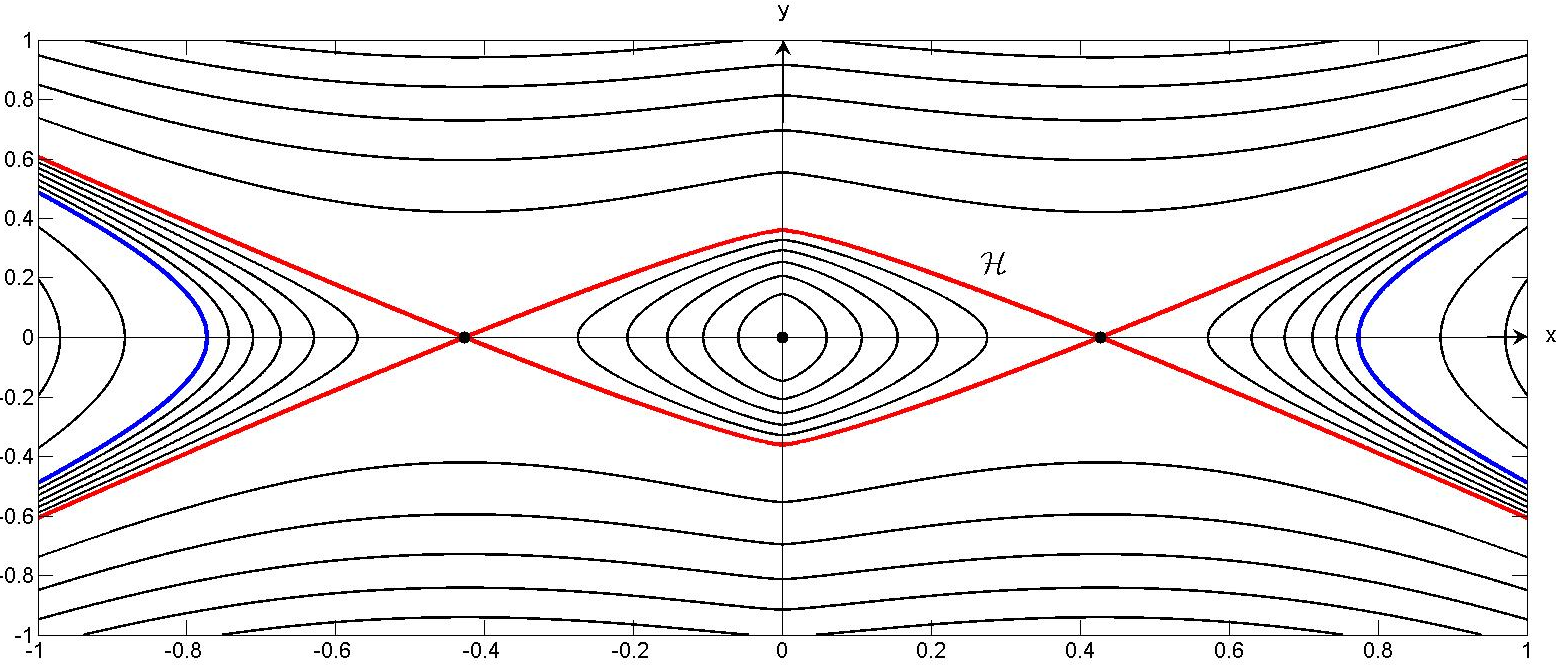
Figure 1: A qualitative sketch of the level curves of $V$

We now focus on the level curves of $V$ on and inside $\cal{H}$, which have

$$0\leq c\leq c^{*}(p),$$ (20)

where

$$c^{*}(p)=\frac{(1-p)^{2/(1-p)}}{2(1+p)}.$$ (21)

These are concentric closed curves surrounding the origin $(0,0)$. We will label the interior of the level curve $V=c$ by $D_{c}$, with the level curve $V=c$ labelled as $\partial D_{c}$, for $0\leq c\leq c^{*}(p)$. In addition, we label the set

$$\bar{D}_{c^{*}(p)}^{\prime}=\bar{D}_{c^{*}(p)}\backslash\{(\pm(1-p)^{1/(1-p)},0),(0,0)\}.$$

Now let $(x^{*}(\eta),y^{*}(\eta))$ be any solution to (S) for $\eta\in[-E,E]$ (any $E>0$) with zero-value $(\alpha,\beta)\in\mathbb{R}^{2}$, and define $F:[-E,E]\to\mathbb{R}$ as,

$$F(\eta)=V(x^{*}(\eta),y^{*}(\eta))\ \ \ \forall\eta\in[-E,E].$$ (22)

Then $F\in C^{1}([-E,E])$, and via (9), (10) and (14),

$$F^{\prime}(\eta)= \nabla V(x^{*}(\eta),y^{*}(\eta)).(x^{*^{\prime}}(\eta),y^{*^{\prime}}(\eta))$$

$$= \nabla V(x^{*}(\eta),y^{*}(\eta)).{\bf{Q}}(x^{*}(\eta),y^{*}(\eta),\eta)\ \ \ \forall\eta\in[-E,E].$$

It then follows, via (18) and (14) that,

$$F^{\prime}(\eta)=-\frac{1}{2}\eta(y^{*}(\eta))^{2}\ \ \ \forall\eta\in[-E,E].$$ (23)

It follows from (23) that

$$F(\eta)\text{ is non-increasing for }\eta\in[0,E],$$ (24)

$$F(\eta)\text{ is non-decreasing for }\eta\in[-E,0].$$ (25)

We can now establish the following,

Lemma 2.

Let $(x^{*}(\eta),y^{*}(\eta))$ be any solution to (S) on $[-E,E]$ (any $E>0$) with zero-value $(\alpha,\beta)\in\bar{D}_{c^{*}(p)}^{\prime}$. Then

$$(x^{*}(\eta),y^{*}(\eta))\in D_{c}\ \ \ \forall\eta\in[-E,E]\backslash\{0\},$$

where $c=V(\alpha,\beta)$.

Proof.

Let the zero-value $(\alpha,\beta)\in\partial D_{c}\backslash\{\pm((1-p)^{\frac{1}{1-p}},0)\}$ with

$$0<c=V(\alpha,\beta)\leq c^{*}(p).$$

We first consider the case when $\beta\not=0$. It follows from (23)-(25) that,

$$F(\eta)<F(0)\ \ \ \forall\eta\in[-E,E]\backslash\{0\}.$$ (26)

Therefore, via (26),

$$V(x^{*}(\eta),y^{*}(\eta))<c\ \ \ \forall\eta\in[-E,E]\backslash\{0\},$$

and so

$$(x^{*}(\eta),y^{*}(\eta))\in D_{c}\ \ \ \forall\eta\in[-E,E]\backslash\{0\},$$

as required. Now consider the case when $\beta=0$. Then $0<|\alpha|<(1-p)^{1/(1-p)}$ and therefore, via (10) $y^{*^{\prime}}(0)\not=0$ after which a similar argument completes the proof. ∎

We now have:

Theorem 3.

For each $(\alpha,\beta)\in\bar{D}_{c^{*}(p)}^{\prime}$, then (S) with zero-value $(\alpha,\beta)$ has a solution $(x^{*}(\eta),y^{*}(\eta))$ on $[-E,E]$ (any $E>0$). Moreover, every such solution satisfies $(x^{*}(\eta),y^{*}(\eta))\in D_{c}$ for all $\eta\in[-E,E]\backslash\{0\}$, where $c=V(\alpha,\beta)$.

Proof.

For any $(\alpha,\beta)\in\bar{D}_{c^{*}(p)}^{\prime}$, Lemma 2 establishes that (S) with zero-value $(\alpha,\beta)$ is a priori bounded. The result then follows by a finite number of applications of the Cauchy-Peano Local Existence Theorem (see [6, Chapter 1, Theorem 1.2]), with $\delta=1/(1+M)$ and

$$M=\max_{(x,y,\eta)\in R^{\prime}}|{\bf{Q}}(x,y,\eta)|$$

whilst

$$R^{\prime}=\{(x,y,\eta)\in\mathbb{R}^{3}:|x|\leq 2(1-p)^{1/(1-p)},\ |y|\leq 2\sqrt{2c^{*}(p)},\ |\eta|\leq 2E\}.$$

The final statement follows immediately from Lemma 2. ∎

We can now establish a global existence result for (S), namely

Corollary 4.

For $(\alpha,\beta)\in\bar{D}_{c^{*}(p)}^{\prime}$ then (S) with zero-value $(\alpha,\beta)$ has a solution $(x^{*}(\eta),y^{*}(\eta))$ on $\mathbb{R}$. Moreover, every such solution satisfies $(x^{*}(\eta),y^{*}(\eta))\in D_{c}$ for all $\eta\in\mathbb{R}\backslash\{0\}$, where $c=V(\alpha,\beta)$.

Proof.

Since Theorem 3 holds for any $E>0$, the result follows immediately. ∎

Remark 2.

Let $(x^{*}(\eta),y^{*}(\eta))$ be any solution to (S) on $[-E,E]$ with zero-value $(0,0)$. It follows from (16), (22) and (23) that

$$V(x^{*}(\eta),y^{*}(\eta))=F(\eta)\leq F(0)=V(0,0)=0\ \ \ \forall\eta\in[-E,E].$$ (27)

Thus $(x^{*}(\eta),y^{*}(\eta))\in\cal{S}$ for all $\eta\in[-E,E]$, with $\cal{S}$ being a connected subset of

$$\{(x,y)\in\mathbb{R}^{2}:V(x,y)\leq 0\}$$

for which $(0,0)\in\cal{S}$. It follows that ${\cal{S}}=\{(0,0)\}$ and so $(x^{*}(\eta),y^{*}(\eta))=(0,0)$ for all $\eta\in[-E,E]$. We conclude that the unique solution to (S) with zero-value $(0,0)$ is given by,

$$(x^{*}(\eta),y^{*}(\eta))=(0,0)\ \ \ \forall\eta\in\mathbb{R}.$$

We next introduce the function $H:\mathbb{R}\to\mathbb{R}$ such that

$$H(x)=\frac{1}{(1-p)}x-x|x|^{p-1}\ \ \ \forall x\in\mathbb{R},$$ (28)

and observe that

$$H\in C(\mathbb{R}).$$ (29)

We have,

Lemma 5.

Let $(\alpha,\beta)\in\bar{D}_{c^{*}(p)}^{\prime}$, and let $(x^{*}(\eta),y^{*}(\eta))$ for $\eta\in\mathbb{R}$ be a global solution to (S) with zero-value $(\alpha,\beta)$. Then

$$y^{*}(\eta)\to 0\text{ as }|\eta|\to\infty.$$

Proof.

We establish the result for $\eta\to\infty$; the result for $\eta\to-\infty$ follows similarly. Now, from (10),

$$y^{*^{\prime}}(\eta)=H(x^{*}(\eta))-\frac{1}{2}\eta y^{*}(\eta)\ \ \ \forall\eta\in[0,\infty).$$ (30)

It then follows from (30) that,

$$y^{*}(\eta)=\beta e^{-\frac{1}{4}\eta^{2}}+e^{-\frac{1}{4}\eta^{2}}\int_{0}^{\eta}H(x^{*}(s))e^{\frac{1}{4}s^{2}}ds\ \ \ \forall\eta\in[0,\infty).$$ (31)

Thus,

$$|y^{*}(\eta)|\leq|\beta|e^{-\frac{1}{4}\eta^{2}}+e^{-\frac{1}{4}\eta^{2}}\int_{0}^{\eta}|H(x^{*}(s))|e^{\frac{1}{4}s^{2}}ds\ \ \ \forall\eta\in[0,\infty).$$ (32)

However, via Corollary 4, $(x^{*}(\eta),y^{*}(\eta))\in\bar{D}_{c^{*}(p)}$ for $\eta\in[0,\infty)$, and so, via (29), there exists a constant $M_{H}\geq 0$ such that

$$|H(x^{*}(s))|\leq M_{H}\ \ \ \forall s\in[0,\infty).$$ (33)

It then follows from (32) and (33) that

$$|y^{*}(\eta)|\leq|\beta|e^{-\frac{1}{4}\eta^{2}}+M_{H}e^{-\frac{1}{4}\eta^{2}}\int_{0}^{\eta}e^{\frac{1}{4}s^{2}}ds\ \ \ \forall\eta\in[0,\infty).$$ (34)

Now a simple application of Watson’s Lemma (see [17, Proposition 2.1]), gives,

$$\int_{0}^{\eta}e^{\frac{1}{4}s^{2}}ds\sim\frac{2}{\eta}e^{\frac{1}{4}\eta^{2}}\text{ as }\eta\to\infty.$$ (35)

We then have, via (34) and (35), that

$$|y^{*}(\eta)|\leq|\beta|e^{-\frac{1}{4}\eta^{2}}+\frac{4M_{H}}{\eta}\text{ as }\eta\to\infty.$$ (36)

It follows from (36) that

$$y^{*}(\eta)\to 0\text{ as }\eta\to\infty,$$

as required ∎

We next have,

Lemma 6.

Let $(x^{*}(\eta),y^{*}(\eta))$ for $\eta\in\mathbb{R}$ be a global solution to (S) with zero-value $(\alpha,\beta)\in\bar{D}_{c^{*}(p)}^{\prime}$, and $F:\mathbb{R}\to\mathbb{R}$ as in (22). Then $F(\eta)$ is non-increasing for $\eta\in(0,\infty)$ and non-decreasing for $\eta\in(-\infty,0)$, with

$$F(\eta)\to\begin{cases}F_{\infty}&\text{ as }\eta\to\infty\\ F_{-\infty}&\text{ as }\eta\to-\infty\end{cases}$$

where $F_{\infty},F_{-\infty}\in[0,F(0))$.

Proof.

We observe from Corollary 4 that

$$(x^{*}(\eta),y^{*}(\eta))\in D_{c}\ \ \ \forall\eta\in\mathbb{R}\backslash\{0\},$$ (37)

with $c=V(\alpha,\beta)=F(0)$, and so,

$$0\leq F(\eta)<F(0)\ \ \ \forall\eta\in\mathbb{R}\backslash\{0\}.$$ (38)

In addition, it follows from (38), (24) and (25), since $F\in C^{1}(\mathbb{R})$, that there exist $F_{\infty},F_{-\infty}\in\mathbb{R}$, such that

$$F(\eta)\to\begin{cases}F_{\infty}&\text{ as }\eta\to\infty\\ F_{-\infty}&\text{ as }\eta\to-\infty\end{cases}$$

where $F_{\infty},F_{-\infty}\in[0,F(0))$, as required. ∎

We now have,

Theorem 7.

Let $(x^{*}(\eta),y^{*}(\eta))$ for $\eta\in\mathbb{R}$ be a global solution to (S) with zero-value $(\alpha,\beta)\in\bar{D}_{c^{*}(p)}^{\prime}$. Then,

$$(x^{*}(\eta),y^{*}(\eta))\to(0,0)\text{ as }|\eta|\to\infty.$$

Proof.

We establish the result for $\eta\to\infty$. The result for $\eta\to-\infty$ follows similarly. We first recall from Corollary 4 that,

$$(x^{*}(\eta),y^{*}(\eta))\in D_{c^{*}(p)}\ \ \ \forall\eta\in\mathbb{R}\backslash\{0\},$$ (39)

and from Lemma 5 that,

$$y^{*}(\eta)\to 0\text{ as }\eta\to\infty.$$ (40)

In addition, we have from Lemma 6 that,

$$V(x^{*}(\eta),y^{*}(\eta))\to F_{\infty}\text{ as }\eta\to\infty$$ (41)

for some $F_{\infty}\in[0,c^{*}(p))$. It follows from (39)-(41) that

$$x^{*}(\eta)\to x_{\infty}\text{ or }x^{*}(\eta)\to-x_{\infty}\text{ as }\eta\to\infty$$ (42)

where $x_{\infty}$ is the single non-negative root of

$$V(x,0)=F_{\infty}\text{ with }x\in[0,(1-p)^{1/(1-p)}).$$

Without loss of generality we will suppose that

$$(x^{*}(\eta),y^{*}(\eta))\to(x_{\infty},0)\text{ as }\eta\to\infty.$$ (43)

However, it follows from (10) that,

$$y^{*}(\eta)=\beta e^{-\frac{1}{4}\eta^{2}}+e^{-\frac{1}{4}\eta^{2}}\int_{0}^{\eta}H(x^{*}(s))e^{\frac{1}{4}s^{2}}ds\ \ \ \eta\in[0,\infty)$$ (44)

with $H:\mathbb{R}\to\mathbb{R}$ given by (28), and

$$H(x_{\infty})\leq 0.$$ (45)

Using (42), it is straightforward to establish that, when,

$$H(x_{\infty})<0,$$ (46)

then from (44),

$$y^{*}(\eta)\sim\frac{2H(x_{\infty})}{\eta}\text{ as }\eta\to\infty.$$ (47)

In addition, from (9), we have,

$$x^{*}(\eta)=\alpha+\int_{0}^{\eta}y^{*}(s)ds\ \ \ \forall\eta\in[0,\infty),$$ (48)

which gives, via (47), that

$$x^{*}(\eta)\sim 2H(x_{\infty})\log{\eta},\ \ \ \text{ as }\eta\to\infty,$$

which contradicts (42). We conclude that (46) cannot hold, and so, via (45), we must have

$$H(x_{\infty})=0,$$ (49)

which, since $x_{\infty}\in[0,(1-p)^{1/(1-p)})$, requires $x_{\infty}=0$. It then follows from (43) that,

$$(x^{*}(\eta),y^{*}(\eta))\to(0,0)\text{ as }\eta\to\infty,$$

as required. ∎

We conclude from Corollary 4 and Theorem 7 that the problem (S) has a two parameter family of nontrivial, distinct homoclinic connections on the equilibrium point $(0,0)$, parametrized by $(\alpha,\beta)\in\bar{D}_{c^{*}(p)}^{\prime}$ which we will denote by $w_{\alpha,\beta}:\mathbb{R}\to\mathbb{R}$ for each $(\alpha,\beta)\in\bar{D}_{c^{*}(p)}^{\prime}$. Here $w=w_{\alpha,\beta}(\eta)$, $\eta\in\mathbb{R}$, has zero-values $w(0)=\alpha$, $w^{\prime}(0)=\beta$. Moreover,

$$(w_{\alpha,\beta}(\eta),w_{\alpha,\beta}^{\prime}(\eta))\in D_{V(\alpha,\beta)}\ \ \ \forall\eta\in\mathbb{R}\backslash\{0\}.$$

Additionally, note that $w_{0,\beta}(\eta)$ is an odd function of $\eta$ whilst $w_{\alpha,0}(\eta)$ is an even function of $\eta$. Furthermore, it also follows from the comments below (13) that $w_{\alpha,\beta}(\eta)$ must be two signed for $\eta\in\mathbb{R}$.

3.2 Decay Bounds and Estimates

In this section, we establish results concerning the rate of decay to zero of $w_{\alpha,\beta}(\eta)$ as $\eta\to\pm\infty$. Specifically, we establish algebraic bounds on the rate of decay of $w_{\alpha,\beta}(\eta)$ as $\eta\to\pm\infty$, and hence, determine that $w_{\alpha,\beta}\in L_{q}(\mathbb{R})$ for each $q>(1-p)/2$. From these bounds we may infer that the corresponding solution to [CP], say $u_{\alpha,\beta}:\mathbb{R}\times[0,\infty)\to\mathbb{R}$, satisfies $u(\cdot,t)\in L_{q}(\mathbb{R})$ for each $t\in[0,\infty)$ and $q>(1-p)/2$. To complement the algebraic bounds, we also provide a rational asymptotic approximation to the decay rate of $w_{\alpha,\beta}(\eta)$ as $\eta\to\pm\infty$, which, in fact suggests exponential decay as $\eta\to\pm\infty$.

To begin, observe that $w=w_{\alpha,\beta}(\eta)$ for $\eta\in\mathbb{R}$, via (6), satisfies

$$(e^{\frac{1}{4}\eta^{2}}w^{\prime})^{\prime}=H(w)e^{\frac{1}{4}\eta^{2}}\ \ \ \forall\eta\in\mathbb{R}.$$

It follows from two successive integrations, that

$$w^{\prime}(\eta)=\beta e^{-\frac{1}{4}\eta^{2}}+e^{-\frac{1}{4}\eta^{2}}\int_{0}^{\eta}H(w(s))e^{\frac{1}{4}s^{2}}ds\ \ \ \forall\eta\in\mathbb{R}$$ (50)

whilst,

$$w(\eta)=\alpha+\int_{0}^{\eta}\beta e^{-\frac{1}{4}t^{2}}dt+\int_{0}^{\eta}e^{-\frac{1}{4}t^{2}}\int_{0}^{t}H(w(s))e^{\frac{1}{4}s^{2}}dsdt\ \ \ \forall\eta\in\mathbb{R}.$$ (51)

We now have,

Proposition 8.

Let $w:\mathbb{R}\to\mathbb{R}$ be a solution to (S) with zero-value $(\alpha,\beta)\in\bar{D}_{c^{*}(p)}^{\prime}$. Suppose that

$$|w(\eta)|\leq\frac{c_{1}}{(1+|\eta|)^{\sigma}}\ \ \ \forall\eta\in\mathbb{R}.$$

with $\sigma\geq 0$ and $c_{1}>0$ (independent of $\alpha$ and $\beta$). Then, there exists $c_{2}>0$, which depends on $c_{1}$, $\sigma$ and $p$, (independent of $\alpha$ and $\beta$) such that,

$$|w^{\prime}(\eta)|\leq\frac{c_{2}}{(1+|\eta|)^{\sigma p+1}}\ \ \ \forall\eta\in\mathbb{R}.$$

Proof.

We give a proof for $\eta\geq 0$; the result for $\eta<0$ follows similarly. Observe that

$$|H(w(\eta))|=\left|\frac{1}{(1-p)}w(\eta)-|w(\eta)|^{p-1}w(\eta)\right|\leq\frac{c_{1}^{p}}{(1+\eta)^{\sigma p}}\ \ \ \forall\eta\in[0,\infty),$$ (52)

since, via Corollary 4, $|w(\eta)|<(1-p)^{\frac{1}{(1-p)}}$ for $\eta\in[0,\infty)$. Thus, via (50) and (52), we have,

$$|w^{\prime}(\eta)|\leq|\beta|e^{-\frac{1}{4}\eta^{2}}+c_{1}^{p}e^{-\frac{1}{4}\eta^{2}}\int_{0}^{\eta}\frac{1}{(1+s)^{\sigma p}}e^{\frac{1}{4}s^{2}}ds\ \ \ \forall\eta\in[0,\infty).$$ (53)

Now, the second term on the right hand side of (53) is a non-negative continuous function for $\eta\in[0,\infty)$, with asymptotic form,

$$c_{1}^{p}e^{-\frac{1}{4}\eta^{2}}\int_{0}^{\eta}\frac{1}{(1+s)^{\sigma p}}e^{\frac{1}{4}s^{2}}ds\sim\frac{2c_{1}^{p}}{\eta^{\sigma p+1}}\text{ as }\eta\to\infty.$$

It follows that,

$$c_{1}^{p}e^{-\frac{1}{4}\eta^{2}}\int_{0}^{\eta}\frac{1}{(1+s)^{\sigma p}}e^{\frac{1}{4}s^{2}}ds\leq\frac{4c_{1}^{p}}{\eta^{\sigma p+1}}\text{ as }\eta\to\infty.$$

We conclude that there exists a positive constant $c_{2}$, depending upon $c_{1}$, $p$, and $\sigma$, such that

$$|w^{\prime}(\eta)|\leq\frac{c_{2}}{(1+\eta)^{\sigma p+1}}\ \ \ \forall\eta\in[0,\infty),$$

as required. ∎

We next have,

Proposition 9.

Let $w:\mathbb{R}\to\mathbb{R}$ be a solution to (S) with zero-value $(\alpha,\beta)\in\bar{D}_{c^{*}(p)}^{\prime}$. Then,

$$(w(\eta),w^{\prime}(\eta))\to(0,0)\text{ as }\eta\to\pm\infty,$$

and moreover,

$$|w^{\prime}(\eta)|\leq\frac{c_{2}}{(1+|\eta|)}\ \ \ \forall\eta\in\mathbb{R},$$

with $c_{2}>0$ dependent upon $p$ (independent of $\alpha$ and $\beta$).

Proof.

The first conclusion follows directly from Theorem 7. Additionally, it follows from Corollary 4 that

$$(w(\eta),w^{\prime}(\eta))\in\mathcal{H}\ \ \ \forall\eta\in\mathbb{R},$$

and hence, it follows from Proposition 8 (with $\sigma=0$, $c_{1}=(1-p)^{1/(1-p)}$) that

$$|w^{\prime}(\eta)|\leq\frac{c_{2}}{(1+|\eta|)}\ \ \ \forall\eta\in\mathbb{R},$$

as required. ∎

We now demonstrate that every solution $w:\mathbb{R}\to\mathbb{R}$ to (S) with zero-value $(\alpha,\beta)\in\bar{D}_{c^{*}(p)}^{\prime}$ decays to zero as $\eta\to\pm\infty$, with decay rate which is at least algebraic in $\eta$ as $\eta\to\pm\infty$. In particular, we demonstrate that $w:\mathbb{R}\to\mathbb{R}$ is contained in $L^{q}(\mathbb{R})$ for any $q>(1-p)/2$. The proof is based on the decay bounds obtained in [10].

Theorem 10.

Let $w:\mathbb{R}\to\mathbb{R}$ be a solution to (S) with zero-value $(\alpha,\beta)\in\bar{D}_{c^{*}(p)}^{\prime}$. Then, for any $\epsilon>0$, there exists $c_{1\epsilon},c_{2\epsilon}>0$ (dependent generally on $\alpha$, $\beta$, $p$ and $\epsilon$) such that

$$|w(\eta)|<\frac{c_{1\epsilon}}{(1+|\eta|)^{\frac{2}{(1-p)}-\epsilon}}\ \ \ \forall\eta\in\mathbb{R},$$

$$|w^{\prime}(\eta)|<\frac{c_{2\epsilon}}{(1+|\eta|)^{\frac{(1+p)}{(1-p)}-\epsilon}}\ \ \ \forall\eta\in\mathbb{R}.$$

Proof.

We give a proof for $\eta\geq 0$; the argument for $\eta<0$ follows similarly. Observe on multiplying (6) by $\eta^{-1}w(\eta)$, we have,

$$\frac{1}{\eta}\left[|w(\eta)|^{1+p}-\frac{(w(\eta))^{2}}{(1-p)}\right]=-\left[\frac{(w(\eta))^{2}}{4}+\frac{w(\eta)w^{\prime}(\eta)}{\eta}\right]^{\prime}+\frac{(w^{\prime}(\eta))^{2}}{\eta}-\frac{w(\eta)w^{\prime}(\eta)}{\eta^{2}}$$ (54)

for $\eta\in(0,\infty)$. Additionally, via Proposition 9, it follows that there exists $\eta_{*}\in(0,\infty)$ such that,

$$|w(\eta)|\leq\left(\frac{2p(1-p)}{(1+p)}\right)^{\frac{1}{(1-p)}}\ \ \ \forall\eta\in[\eta_{*},\infty),$$ (55)

and for $F:[0,\infty)\to\mathbb{R}$ given by

$$F(\eta)=V(w(\eta),w^{\prime}(\eta))\ \ \ \forall\eta\in[0,\infty),$$

that

$$0\leq F(\eta)\leq\left(\frac{4(c(p))^{\frac{2}{(1+p)}}}{C(p)}\right)^{(1+p)/(1-p)}\ \ \ \eta\in[\eta_{*},\infty),$$ (56)

where

$$c(p)=\frac{1}{(1+p)}-\frac{1}{2},\text{ and }C(p)=\frac{2(1+p)}{(1-p)}+1.$$ (57)

Thus, it follows from (54) that

$$\frac{F(\eta)}{\eta} =\frac{(w^{\prime}(\eta))^{2}}{2\eta}+\frac{1}{\eta}\left[-\frac{(w(\eta))^{2}}{2(1-p)}+\frac{|w(\eta)|^{1+p}}{(1+p)}\right]$$

$$\leq\frac{(w^{\prime}(\eta))^{2}}{2\eta}+\frac{1}{\eta}\left[-\frac{(w(\eta))^{2}}{(1-p)}+|w(\eta)|^{1+p}\right]$$

$$=\frac{3(w^{\prime}(\eta))^{2}}{2\eta}-\left[\frac{(w(\eta))^{2}}{4}+\frac{w(\eta)w^{\prime}(\eta)}{\eta}\right]^{\prime}-\frac{w(\eta)w^{\prime}(\eta)}{\eta^{2}},$$ (58)

for $\eta\in[\eta_{*},\infty)$. Since $F(\eta)\geq 0$ for all $\eta\in[\eta^{*},\infty)$, together with the decay estimates in Proposition 9, it follows that we may integrate inequality (58) from $\eta\ (\geq\eta^{*})$ to $l$, and then allow $l\to\infty$, to obtain,

$$\int_{\eta}^{\infty}\frac{F(t)}{t}dt\leq\frac{(w(\eta))^{2}}{4}+\frac{2}{\eta}\sup_{t\geq\eta}|w(t)w^{\prime}(t)|+\frac{3}{2}\int_{\eta}^{\infty}\frac{(w^{\prime}(t))^{2}}{t}dt$$ (59)

for $\eta\in[\eta_{*},\infty)$. We also note, that since, via Corollary 4, $|w(\eta)|<(1-p)^{1/(1-p)}$, we have,

$$F(\eta)\geq|w(\eta)|^{1+p}c(p)\geq 0,$$ (60)

for $\eta\in[\eta_{*},\infty)$. It therefore follows from (59) and (60) that

$$0\leq\int_{\eta}^{\infty}\frac{F(t)}{t}dt\leq\frac{1}{4}\left(\frac{F(\eta)}{c(p)}\right)^{\frac{2}{(1+p)}}+\frac{2}{\eta}\sup_{t\geq\eta}|w(t)w^{\prime}(t)|+\frac{3}{2}\int_{\eta}^{\infty}\frac{(w^{\prime}(t))^{2}}{t}dt$$ (61)

for $\eta\in[\eta_{*},\infty)$. We observe that the right hand side of (61) is uniformly bounded for $\eta\in[\eta_{*},\infty)$ via Proposition 9.

Now suppose that there exists $k>0$ such that

$$F(\eta)\leq\frac{k}{\eta^{\sigma}}\ \ \ \forall\eta\in[\eta_{*},\infty)$$ (62)

for some $\sigma\geq 0$ (note that (62) holds when $\sigma=0$ via Proposition 9). Then, via (60), it follows that there exists $c_{1}>0$ such that

$$|w(\eta)|\leq\frac{c_{1}}{\eta^{\frac{\sigma}{(1+p)}}}\ \ \ \forall\eta\in[\eta_{*},\infty)$$ (63)

and so, via Proposition 8, there exists $c_{2}>0$ such that

$$|w^{\prime}(\eta)|\leq\frac{c_{2}}{\eta^{\frac{\sigma p}{(1+p)}+1}}\ \ \ \forall\eta\in[\eta_{*},\infty).$$ (64)

Thus, it follows from (61)-(64) and (56), that there exists $c_{3},c_{4},c_{5}>0$ such that

$$\int_{\eta}^{\infty}\frac{F(t)}{t}dt \leq\frac{1}{4}\left(\frac{F(\eta)}{c(p)}\right)^{\frac{2}{(1+p)}}+\frac{c_{3}}{\eta^{\sigma+2}}+\frac{c_{4}}{\eta^{\frac{2\sigma p}{(1+p)}+2}}$$

$$\leq\frac{F(\eta)}{C(p)}+\frac{c_{5}}{\eta^{\frac{2\sigma p}{(1+p)}+2}}$$ (65)

for $\eta\in[\eta_{*},\infty)$. Upon setting $G:[\eta_{*},\infty)\to\mathbb{R}$ to be

$$G(\eta)=\int_{\eta}^{\infty}\frac{F(t)}{t}dt\ \ \ \forall\eta\in[\eta_{*},\infty),$$

it follows from (65) that $G$ satisfies,

$$\left(t^{C(p)}G(t)\right)^{\prime}\leq\frac{c_{6}}{t^{\frac{2\sigma p}{(1+p)}+3-C(p)}}\ \ \ \forall t\in[\eta_{*},\infty),$$ (66)

with $c_{6}>0$ constant. An integration of (66) gives

$$G(\eta)\leq\frac{c_{7}}{\eta^{\frac{2\sigma p}{(1+p)}+2}}+\frac{c_{8}}{\eta^{C(p)}}\ \ \ \forall\eta\in[\eta_{*},\infty),$$ (67)

with $c_{7},c_{8}>0$ constants. Also, recalling, via Lemma 6, that $F(\eta)$ is non-increasing on $[\eta^{*},\infty)$, we have,

$$G(\eta)\geq\int_{\eta}^{2\eta}\frac{F(t)}{t}dt\geq\frac{1}{2}F(2\eta),\ \ \ \forall\eta\in[\eta_{*},\infty).$$ (68)

Thus, it follows from (67) and (68) that there exist constants $c_{9},c_{10}>0$ such that

$$F(\eta)\leq\frac{c_{9}}{\eta^{\frac{2\sigma p}{(1+p)}+2}}+\frac{c_{10}}{\eta^{C(p)}}\ \ \ \forall\eta\in[\eta_{*},\infty).$$ (69)

Since (62) holds for $\sigma=0$, it follows that there exists sequences $\{\sigma_{n}\}_{n\in\mathbb{N}}$ and $\{k_{n}\}_{n\in\mathbb{N}}$ given by

$$\sigma_{1}=0,\ \ \ \sigma_{n+1}=\min\left\{\frac{2\sigma_{n}p}{(1+p)}+2,\ C(p)\right\}$$ (70)

such that

$$F(\eta)\leq\frac{k_{n}}{\eta^{\sigma_{n}}}\ \ \ \forall\eta\in[\eta_{*},\infty).$$ (71)

We obtain from (70) and (57) that,

$$\sigma_{n}=\frac{2(1+p)}{(1-p)}-\frac{4p}{(1-p)}\left(\frac{2p}{(1+p)}\right)^{n-2}\ \ \ \forall n\in\mathbb{N}$$

and hence $\sigma_{n}$ is increasing with

$$\sigma_{n}\to\frac{2(1+p)}{(1-p)}\ \ \ \text{ as }n\to\infty.$$ (72)

Therefore it follows, via (60) and (70)-(72), that for each $\epsilon>0$ there exists $c_{1\epsilon}>0$ such that

$$|w(\eta)|\leq\frac{c_{1\epsilon}}{(1+\eta)^{\frac{2}{(1-p)}-\epsilon}}\ \ \ \forall\eta\in[0,\infty),$$ (73)

recalling that $w(\eta)$ is bounded on $[0,\eta^{*}]$. The bound on $|w^{\prime}(\eta)|$ follows immediately from (73) and Proposition 8. ∎

The algebraic bounds in Theorem 10 are the tightest decay rates we have been able to establish rigorously. However, the following asymptotic argument indicates that, in fact, $w=w_{\alpha,\beta}(\eta)$ decays exponentially in $\eta$ as $|\eta|\to\infty$, accompanied by rapid oscillatory behaviour. To this end, we now consider the asymptotic structure of $w=w_{\alpha,\beta}(\eta)$ as $\eta\to\infty$, with the same structure following as $\eta\to-\infty$. Now, for $\eta>>1$, then $w=w_{\alpha,\beta}(\eta)$ satisfies,

$$w^{\prime\prime}+\frac{1}{2}\eta w^{\prime}+w|w|^{p-1}-\frac{1}{(1-p)}w=0\ \ \ \eta>>1$$ (74)

$$w(\eta),\ w^{\prime}(\eta)\to 0\ \ \ \text{ as }\eta\to\infty,$$ (75)

via (6) and Proposition 9. On using (75), the dominant form of (74) when $\eta>>1$ is

$$w^{\prime\prime}+w|w|^{p-1}=0.$$ (76)

Every solution to (76) is periodic and may be written (up to translation in $\eta$) as,

$$w(\eta,a)=aW\left(a^{-\frac{1}{2}(1-p)}\eta\right),\ \ \ \forall\eta\in\mathbb{R},$$ (77)

where $a\in\mathbb{R}^{+}$ is a parameter and $W:\mathbb{R}\to\mathbb{R}$ is that unique periodic function which satisfies the problem,

$$W^{\prime\prime}+W|W|^{p-1}=0,\ \ \ \zeta\in\mathbb{R}$$ (78)

$$W(0)=1,\ \ \ W^{\prime}(0)=0.$$ (79)

The period of $W(\zeta)$ is given by

$$T(p)=2^{3/2}(1+p)^{1/2}\int_{0}^{1}\frac{d\lambda}{(1-\lambda^{(1+p)})^{1/2}}$$ (80)

whilst,

$$W(\zeta)=-W\left(\frac{1}{2}T(p)-\zeta\right)=W(-\zeta)\ \ \ \forall\zeta\in\mathbb{R}.$$ (81)

Via an integration, the solution to (78)-(79) satisfies

$$\frac{(W^{\prime}(\eta))^{2}}{2}+\frac{|W(\eta)|^{1+p}}{(1+p)}=\frac{1}{(1+p)}\ \ \ \forall\eta\in\mathbb{R},$$

which represents a periodic orbit in the $(W,W^{\prime})$ phase plane, as illustrated in Figure 2. It follows from (77) that $w(\eta,a)$ has amplitude $a>0$ and period

$$T_{a}(p)=a^{\frac{1}{2}(1-p)}T(p).$$ (82)

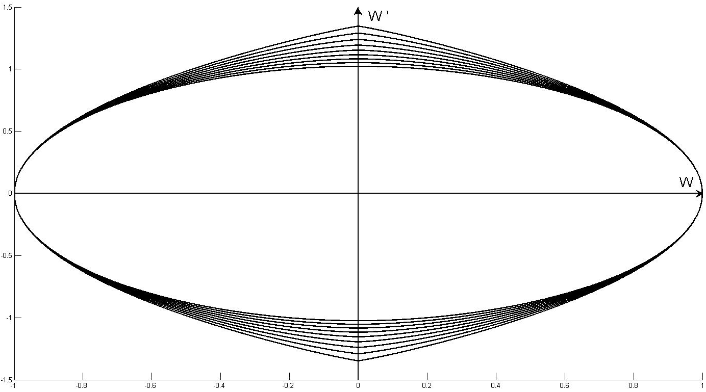
Figure 2: Phase paths for solutions to (78)-(79) for $p_{k}=(0.1)k$ for $k=1...9$. Here the phase path for $p_{k}$ encloses the phase path for $p_{k+1}$ for $k=1...8$.

For any fixed $a\in\mathbb{R}^{+}$, (77) cannot represent the asymptotic structure to (74) and (75) since $W$ is periodic. The remaining terms in (74) must induce decay as $\eta\to\infty$. However, we observe from (82) that the oscillations in $w(\eta,a)$ becomes increasingly rapid as the amplitude $a\to 0^{+}$. This suggests that we seek the asymptotic structure of (74)-(75) as $\eta\to\infty$ in the form,

$$w(\eta)\sim a(\eta)W(a(\eta)^{-\frac{1}{2}(1-p)}\eta)\text{ as }\eta\to\infty,$$ (83)

with $a(\eta)>0$ and,

$$a(\eta),a^{\prime}(\eta)\to 0\text{ as }\eta\to\infty.$$ (84)

Now, the rate of change of amplitude of oscillation in (83), $a^{\prime}(\eta)$, approaches zero as $\eta\to\infty$, whilst the frequency of oscillation becomes unbounded as $\eta\to\infty$. We can thus use an averaging approach to determine an evolution equation for the amplitude $a(\eta)$ as $\eta\to\infty$. We substitute (83) into (6) and make use of (78). We then integrate the resulting ordinary differential equation over one period of $W(\cdot)$, over which, we may hold $a$ fixed. We obtain the leading order amplitude equation as,

$$a^{\prime\prime}+\frac{1}{2}\eta a^{\prime}-\frac{1}{(1-p)}a=0,\ \ \ \eta>>1,$$ (85)

$$a(\eta),a^{\prime}(\eta)\to 0\text{ as }\eta\to\infty.$$ (86)

The linear ordinary differential equation (85) has two basis functions $a_{+}:\mathbb{R}\to\mathbb{R}$ and $a_{-}:\mathbb{R}\to\mathbb{R}$ which have

$$a_{+}(\eta)\sim\eta^{-\left(1+\frac{2}{(1-p)}\right)}e^{-\frac{1}{4}\eta^{2}},\ \ \ a_{-}(\eta)\sim\eta^{\frac{2}{(1-p)}}\ \ \ \text{ as }\eta\to\infty.$$

It follows that

$$a(\eta)\sim A_{\infty}\eta^{-\left(1+\frac{2}{(1-p)}\right)}e^{-\frac{1}{4}\eta^{2}}\ \ \ \text{ as }\eta\to\infty,$$ (87)

with $A_{\infty}$ being a positive globally determined constant dependent, in general, on $\alpha$, $\beta$ and $p$. Thus, from (83), we have

$$w_{\alpha,\beta}(\eta)\sim a(\eta)W(a(\eta)^{-\frac{1}{2}(1-p)}\eta)\text{ as }\eta\to\infty,$$ (88)

with, $\alpha(\eta)$ having the asymptotic form (87) as $\eta\to\infty$. The same argument leads to the same (up to the constant $A_{\infty}$) asymptotic structure as $\eta\to-\infty$. As a consequence of (87) and (88), we anticipate that $w_{\alpha,\beta}(\eta)$ decays to zero at a Gaussian rate as $|\eta|\to\infty$, whilst oscillating about zero with a local frequency which increases at a Gaussian rate as $|\eta|\to\infty$. This indicates that, in fact, $w_{\alpha,\beta}\in L^{q}(\mathbb{R})$ for any $q>0$.

3.3 Localized Solutions to [CP]

Following Corollary 4 and Theorem 7, for each $(\alpha,\beta)\in\bar{D}_{c^{*}(p)}^{\prime}$, we have constructed a non-trivial, localized, global solution $u_{\alpha,\beta}:\mathbb{R}\times[0,\infty)\to\mathbb{R}$ to [CP], namely,

$$u_{\alpha,\beta}(x,t)=\begin{cases}t^{\frac{1}{(1-p)}}w_{\alpha,\beta}\left(\frac{x}{t^{1/2}}\right)&,(x,t)\in\mathbb{R}\times(0,\infty)\\ 0&,(x,t)\in\mathbb{R}\times\{0\}.\end{cases}$$ (89)

With this two parameter family of solutions to [CP], each solution is distinct, and is not a spatial translate of any other solution in the family. However, we observe that $u_{\alpha,\beta}(x-x_{0},t)$ is also a global solution to [CP] for any fixed $x_{0}\in\mathbb{R}$. A trivial calculation from (89) establishes that

$$(u_{\alpha,\beta})_{x}(x,t)=t^{\frac{1}{(1-p)}-\frac{1}{2}}w_{\alpha,\beta}^{\prime}\left(\frac{x}{t^{1/2}}\right),$$ (90)

$$(u_{\alpha,\beta})_{t}(x,t)=\frac{1}{(1-p)}t^{\frac{1}{(1-p)}-1}\left(w_{\alpha,\beta}\left(\frac{x}{t^{1/2}}\right)-\frac{1}{2}(1-p)\left(\frac{x}{t^{1/2}}\right)w_{\alpha,\beta}^{\prime}\left(\frac{x}{t^{1/2}}\right)\right),$$ (91)

for $(x,t)\in\mathbb{R}\times(0,\infty)$, whilst from (1),

$$(u_{\alpha,\beta})_{xx}(x,t)=(u_{\alpha,\beta})_{t}(x,t)-(u_{\alpha,\beta}|u_{\alpha,\beta}|^{p-1})(x,t),$$ (92)

for $(x,t)\in\mathbb{R}\times(0,\infty)$. It then follows immediately from Theorem 7 that,

$$(u_{\alpha,\beta})_{x},\ (u_{\alpha,\beta})_{t},\ (u_{\alpha,\beta})_{xx}\to 0\text{ as }t\to 0^{+}\text{ uniformly for }x\in\mathbb{R},$$

and so, in fact,

$$u_{\alpha,\beta}\in L^{\infty}(\mathbb{R}\times[0,T])\cap C(\mathbb{R}\times[0,T])\cap C^{2,1}(\mathbb{R}\times[0,T]).$$ (93)

It follows from (93) that for each $(\alpha,\beta)\in\bar{D}_{c^{*}(p)}^{\prime}$, and any $\tau>0$, then $u_{\alpha,\beta}^{\tau}:\mathbb{R}\times[0,\infty)\to\mathbb{R}$ such that

$$u_{\alpha,\beta}^{\tau}(x,t)=\begin{cases}(t-\tau)^{\frac{1}{(1-p)}}w_{\alpha,\beta}\left(\frac{x}{(t-\tau)^{1/2}}\right)&,(x,t)\in\mathbb{R}\times(\tau,\infty)\\ 0&,(x,t)\in\mathbb{R}\times[0,\tau]\end{cases}$$

is also a non-trivial, localized, global solution to [CP]. Finally, we observe, via Theorem 10 that for each $q>(1-p)/2$, then $u_{\alpha,\beta}(\cdot,t)\in L^{q}(\mathbb{R}$ for each $t\geq 0$. Moreover, (87) and (88) suggest that the localization is Gaussian in $x$ for each $t>0$.

4 Heteroclinic Connections

In this section we establish the existence of at least one heteroclinic connection for (S) from the equilibrium point $(-(1-p)^{1/(1-p)},0)$ to the equilibrium point $((1-p)^{1/(1-p)},0)$.

4.1 Existence

We first consider solutions to the problem (S) for $\eta\in[0,\infty)$ and which remain in the region $\Omega\subset\mathbb{R}^{2}$, given as

$$\Omega=\left\{(x,y):0<x<(1-p)^{1/(1-p)},y>0\right\}$$ (94)

with boundary $\partial\Omega=\overline{\Omega}\ \backslash\ \Omega$. We also define the following subset of $\partial\Omega$, namely,

$$\partial\Omega_{1}=\left\{(x,y):x=0,y>0\right\}.$$ (95)

Specifically, we consider (S) for $\eta\in[0,\infty)$ and demonstrate that there exists a solution $(x,y):[0,\infty)\to\overline{\Omega}$ with zero-value $(0,\beta)\in\partial\Omega_{1}$ and which satisfies

$$(x(\eta),y(\eta))\in\Omega\ \ \ \forall\eta\in(0,\infty),$$ (96)

$$(x(\eta),y(\eta))\to((1-p)^{1/(1-p)},0)\ \ \ \text{ as }\eta\to\infty.$$ (97)

To begin with, it is readily established that for each zero-value $(0,\beta)\in\partial\Omega_{1}$, then (S) has a local solution $(x,y):[0,\delta]\to\mathbb{R}^{2}$ (for some $\delta>0$). Moreover, $(x(\eta),y(\eta))\in\Omega$ for $\eta\in(0,\delta]$, and $x(\eta)$ is monotone increasing whilst $y(\eta)$ is monotone decreasing, with $\eta\in(0,\delta]$. It is then straightforward to establish that $(x(\eta),y(\eta))$ can be uniquely continued beyond $\eta=\delta$ and must satisfy one of the following three possibilities:

1. There exists $\eta_{\beta}>0$ such that $(x(\eta),y(\eta))\in\Omega$ for all $\eta\in(0,\eta_{\beta})$ and $(x(\eta_{\beta}),y(\eta_{\beta}))=((1-p)^{\frac{1}{1-p}},y_{\beta})$ with $0<y_{\beta}<\beta$, whilst $x^{\prime}(\eta_{\beta})=y_{\beta}>0$, and so there exists $\epsilon_{\beta}>0$ such that $(x(\eta),y(\eta))\not\in\bar{\Omega}\cup(\{0\}\times\mathbb{R})$ for $\eta\in(\eta_{\beta},\eta_{\beta}+\epsilon_{\beta}]$.

2. There exists $\eta_{\beta}>0$ such that $(x(\eta),y(\eta))\in\Omega$ for all $\eta\in(0,\eta_{\beta})$ and $(x(\eta_{\beta}),y(\eta_{\beta}))=(x_{\beta},0)$ with $0<x_{\beta}<(1-p)^{\frac{1}{1-p}}$, whilst $y^{\prime}(\eta_{\beta})<0$ and so there exists $\epsilon_{\beta}>0$ such that $(x(\eta),y(\eta))\not\in\bar{\Omega}\cup(\{0\}\times\mathbb{R})$ for $\eta\in(\eta_{\beta},\eta_{\beta}+\epsilon_{\beta}]$.

3. $(x(\eta),y(\eta))\in\Omega$ for all $\eta\in(0,\infty)$ and $(x(\eta),y(\eta))\to((1-p)^{\frac{1}{1-p}},0)$ as $\eta\to\infty$.

Our aim now is to obtain a uniqueness result for (S) with zero-value in $\partial\Omega_{1}$, and from this a continuous dependence result. This is non-trivial, since $\bf{Q}$ in (14) is not locally Lipschitz continuous in any neighborhood of $(0,\beta)\in\partial\Omega_{1}$, and so standard uniqueness and continuous dependence theory fail to apply. To begin with, we provide a local a priori bound for any solution of (S) with zero-value $(0,\beta)\in\partial\Omega_{1}$.

Proposition 11.

Let $(x,y):[0,\eta_{\beta}]\to\mathbb{R}^{2}$ be any solution to (S) with zero-value $(0,\beta)\in\partial\Omega_{1}$ and which satisfies either case (i) or (ii). Then,

$$\eta_{\beta}>\min\left\{\left(\frac{2}{\beta}\right)\left(m_{H}+\sqrt{m_{H}^{2}+\frac{(\beta)^{2}}{2}}\right),\ \frac{(1-p)^{1/(1-p)}}{\beta}\right\}=\eta^{*}$$ (98)

with

$$m_{H}=\inf_{\lambda\in[0,(1-p)^{1/(1-p)}]}H(\lambda),$$ (99)

Proof.

Let $(x,y):[0,\eta_{\beta}]\to\mathbb{R}^{2}$ be any solution to (S) with zero-value $(0,\beta)\in\partial\Omega_{1}$, and which satisfies either case (i) or case (ii). Suppose that $\eta_{\beta}\leq\eta^{*}$. Since $(x(\eta),y(\eta))\in\Omega$ for all $\eta\in(0,\eta_{\beta})$, it follows from (10) that

$$\beta+m_{H}\eta-\frac{\beta}{4}\eta^{2}<y(\eta)<\beta\ \ \ \forall\eta\in(0,\eta_{\beta}].$$ (100)

However, $\eta_{\beta}\leq\eta^{*}$ and so, via (100),

$$\frac{\beta}{2}<y(\eta)<\beta\ \ \ \forall\eta\in(0,\eta_{\beta}].$$ (101)

An integration of (9) using (101), then gives,

$$\frac{\beta\eta}{2}<x(\eta)<\beta\eta\ \ \ \forall\eta\in(0,\eta_{\beta}].$$ (102)

It finally follows from (101) and (102), since $\eta_{\beta}\leq\eta^{*}$, that,

$$x(\eta_{\beta})<\beta\eta_{\beta}\leq\beta\eta^{*}\leq(1-p)^{\frac{1}{1-p}},\ \ \ y(\eta_{\beta})>\frac{\beta}{2},$$

and so $(x(\eta_{\beta}),y(\eta_{\beta}))\in\Omega$, which is a contradiction. We conclude that $\eta_{\beta}>\eta^{*}$, as required. ∎

Therefore, we have,

Corollary 12.

Let $(x,y):[0,\eta^{*}]\to\mathbb{R}^{2}$ be a solution to (S) with zero-value $(0,\beta)\in\partial\Omega_{1}$ with $\eta^{*}$ given by (98). Then,

$$\frac{\beta\eta}{2}<x(\eta)<(1-p)^{1/(1-p)},\ \ \ \frac{\beta}{2}<y(\eta)<\beta\ \ \ \forall\eta\in[0,\eta^{*}],$$

Proof.

For cases (i) and (ii), the result follows from Proposition 11, with case (iii) following immediately. ∎

The a priori bounds in Corollary 12, allow us to establish the following local uniqueness result for (S) with zero-value $(0,\beta)\in\partial\Omega_{1}$. The proof is based on the uniqueness argument in [1].

Proposition 13.

The problem (S) with zero-value $(0,\beta)\in\partial\Omega_{1}$ has at most one solution on $[0,\eta^{*}]$, with $\eta^{*}>0$ given by (98).

Proof.

To begin, fix $(0,\beta)\in\partial\Omega_{1}$. Suppose that $(x,y),(x^{*},y^{*}):[0,\eta^{*}]\to\mathbb{R}^{2}$ are solutions to (S) with zero-value $(0,\beta)$. It follows from Corollary 12 that

$$(x(\eta),y(\eta)),(x^{*}(\eta),y^{*}(\eta))\in\bar{\Omega}\ \ \ \forall\eta\in[0,\eta^{*}],$$ (103)

whilst from Corollary 12,

$$|x(\eta)-x^{*}(\eta)|<(1-p)^{1/(1-p)},\ \ \ |y(\eta)-y^{*}(\eta)|<\beta\ \ \ \forall\eta\in[0,\eta^{*}].$$ (104)

Additionally, we observe that for $(X,Y)\in[0,(1-p)^{1/(1-p)}]\times[0,\beta]$, then

$$X+X^{p}+Y<\left(2+\beta^{1-p}\right)(X+Y)^{p},$$ (105)

since $0<p<1$. Now, via (9) and (10) respectively, we have,

$$|x(\eta)-x^{*}(\eta)|\leq\int_{0}^{\eta}|y(s)-y^{*}(s)|ds$$ (106)

$$|y(\eta)-y^{*}(\eta)|\leq\int_{0}^{\eta}\left(\frac{1}{(1-p)}|x(s)-x^{*}(s)|+|x(s)-x^{*}(s)|^{p}+\frac{s}{2}|y(s)-y^{*}(s)|\right)ds$$ (107)

for all $\eta\in[0,\eta^{*}]$. We next introduce $v:[0,\eta^{*}]\to\mathbb{R}$ as,

$$v(\eta)=|x(\eta)-x^{*}(\eta)|+|y(\eta)-y^{*}(\eta)|\ \ \ \forall\eta\in[0,\eta^{*}].$$ (108)

Therefore, via (103)-(108), it follows that

$$v(\eta)\leq \int_{0}^{\eta}\left(\frac{1}{(1-p)}|x(s)-x^{*}(s)|+|x(s)-x^{*}(s)|^{p}+\left(\frac{s}{2}+1\right)|y(s)-y^{*}(s)|\right)ds$$

$$\leq \int_{0}^{\eta}\frac{1}{(1-p)}\left(\frac{\eta^{*}}{2}+1\right)\left(|x(s)-x^{*}(s)|+|x(s)-x^{*}(s)|^{p}+|y(s)-y^{*}(s)|\right)ds$$

$$\leq \int_{0}^{\eta}\frac{1}{(1-p)}\left(\frac{\eta^{*}}{2}+1\right)(2+\beta^{1-p})\left(v(s)\right)^{p}ds$$ (109)

for all $\eta\in[0,\eta^{*}]$, where the final inequality is due to (104) and (105). Also, via Corollary 12 and (98), $\eta^{*}$ is dependent on $p$ and $\beta$ only, and hence, it follows from (109) that

$$v(\eta)\leq\int_{0}^{\eta}K(p,\beta)\left(v(s)\right)^{p}ds$$ (110)

for all $\eta\in[0,\eta^{*}]$, where the constant $K(p,\beta)$ is given by,

$$K(p,\beta)=\frac{1}{(1-p)}\left(\frac{\eta^{*}}{2}+1\right)(2+\beta^{1-p}).$$

We now introduce the function $\bar{H}:[0,\eta^{*}]\to\overline{\mathbb{R}}_{+}$ given by,

$$\bar{H}(\eta)=\int_{0}^{\eta}K(p,\beta)\left(v(s)\right)^{p}ds\ \ \ \forall\eta\in[0,\eta^{*}].$$ (111)

It follows from (111) that $\bar{H}$ is non-negative, non-decreasing and differentiable on $[0,\eta^{*}]$, and via (110), satisfies

$$(\bar{H}(s))^{\prime}\leq K(p,\beta)(\bar{H}(s))^{p}\ \ \ \forall s\in[0,\eta^{*}].$$ (112)

Upon integrating (112) from $0$ to $\eta$, we obtain

$$\bar{H}(\eta)\leq((1-p)K(p,\beta)\eta)^{1/(1-p)}\ \ \ \forall\eta\in[0,\eta^{*}]$$ (113)

and it follows from (113), (111) and (110) that

$$v(\eta)\leq\delta\ \ \ \forall\eta\in\left[0,\eta_{\delta}\right],$$ (114)

where $\delta>0$ is chosen sufficiently small so that

$$\eta_{\delta}=\frac{\delta^{1-p}}{(1-p)K(p,\beta)}<\eta^{*}.$$

Now, from Corollary 12, we have

$$\min\{x^{*}(\eta),x(\eta)\}\geq\frac{\beta\eta}{2}\ \ \ \forall\eta\in[0,\eta^{*}].$$ (115)

Moreover, it follows from (14), (115) and the mean value theorem, that there exists $\theta(s)\geq\min\{x^{*}(s),x(s)\}$, for which,

$$|Q_{2}(x(s) ,y(s),s)-Q_{2}(x^{*}(s),y^{*}(s),s)|$$

$$\leq\frac{1}{(1-p)}|x(s)-x^{*}(s)|+|x(s)^{p}-x^{*}(s)^{p}|+\frac{s}{2}|y(s)-y^{*}(s)|$$

$$\leq\frac{1}{(1-p)}|x(s)-x^{*}(s)|+p(\theta(s))^{p-1}|x(s)-x^{*}(s)|+\frac{\eta^{*}}{2}|y(s)-y^{*}(s)|$$

$$\leq\left(\frac{1}{(1-p)}+p\left(\frac{\beta s}{2}\right)^{p-1}\right)|x(s)-x^{*}(s)|+\frac{\eta^{*}}{2}|y(s)-y^{*}(s)|$$

$$\leq\left(\frac{1}{(1-p)}+p\left(\frac{\beta s}{2}\right)^{p-1}+\frac{\eta^{*}}{2}\right)v(s)$$ (116)

for all $s\in(0,\eta^{*}]$. Now, via (9), (10), (14), (105), (116) and (114), we have,

$$v(\eta)\leq \int_{0}^{\eta}\left(|Q_{1}(x(s),y(s),s)-Q_{1}(x^{*}(s),y^{*}(s),s)|\right.$$

$$\ \ \ \ \ +\left.|Q_{2}(x(s),y(s),s)-Q_{2}(x^{*}(s),y^{*}(s),s)|\right)ds$$

$$\leq \int_{0}^{\eta_{\delta}}K(p,\beta)(v(s))^{p}ds+\int_{\eta_{\delta}}^{\eta}\left(1+\frac{1}{(1-p)}+p\left(\frac{\beta s}{2}\right)^{p-1}+\frac{\eta^{*}}{2}\right)v(s)ds$$

$$\leq \frac{\delta}{(1-p)}+\int_{\eta_{\delta}}^{\eta}\left(1+\frac{1}{(1-p)}+p\left(\frac{\beta s}{2}\right)^{p-1}+\frac{\eta^{*}}{2}\right)v(s)ds$$ (117)

for all $\eta\in[\eta_{\delta},\eta^{*}]$. An application of Gronwall’s Lemma [2, Corollary 6.2] to (117), gives

$$v(\eta)\leq\frac{\delta}{(1-p)}e^{\left(\eta^{*}\left(1+\frac{1}{(1-p)}+\left(\frac{\beta\eta^{*}}{2}\right)^{p-1}+\frac{\eta^{*}}{2}\right)\right)}$$ (118)

for all $\eta\in[\eta_{\delta},\eta^{*}]$. Since $v$ is non-negative and $\eta^{*}$ is independent of $\delta$, it follows from (118) and (114), upon letting $\delta\to 0$, that

$$v(\eta)=0\ \ \ \forall\eta\in[0,\eta^{*}].$$ (119)

Finally, it follows from (119) and (108) that

$$(x(\eta),y(\eta))=(x^{*}(\eta),y^{*}(\eta))\ \ \ \forall\eta\in[0,\eta^{*}],$$

as required. ∎

We can now state the following uniqueness result.

Lemma 14.

For each $(0,\beta)\in\partial\Omega_{1}$ then (S) with zero-value $(0,\beta)$ has exactly one solution $(x,y):I\to\mathbb{R}^{2}$. This solution satisfies exactly one of the cases: (i) (with $I=[0,\eta_{\beta}+\epsilon_{\beta}]$), (ii) (with $I=[0,\eta_{\beta}+\epsilon_{\beta}]$) or (iii) (with $I=[0,\infty)$).

Proof.

We have established earlier that for each $(0,\beta)\in\partial\Omega_{1}$, then (S) with zero-value $(0,\beta)$ has at least one solution $(x,y):I\to\mathbb{R}^{2}$, and that the solution satisfies one of the cases (i)-(iii). It follows from Proposition 13 that this solution is unique for $\eta\in[0,\eta^{*}]$, (with $\eta^{*}$ depending only upon $\beta$ and $p$) and, moreover, in whichever case of (i)-(iii) it falls, that $(x(\eta),y(\eta))\not\in\{(0,\lambda):\lambda\in\mathbb{R}\}$ for any $\eta\in I\ \backslash\ [0,\eta^{*}]$. Repeated application of the classical uniqueness theorem [6, Chapter 1, Theorem 2.2] then completes the uniqueness result for $\eta\in I\ \backslash\ [0,\eta^{*}]$. ∎

We immediately obtain a continuous dependence result for solutions of (S) with zero-value in $\partial\Omega_{1}$, namely,

Corollary 15.

Let $(0,\beta^{*})\in\partial\Omega_{1}$ and suppose that the unique solution to (S) with zero-value $(0,\beta^{*})$, say $(x^{*},y^{*}):I\to\mathbb{R}$, satisfies case (i) or (ii), with $I=[0,\eta_{\beta^{*}}+\epsilon_{\beta^{*}}]$. Then, given $\epsilon^{\prime}>0$, there exists $\delta^{\prime}>0$ such that for all $\beta>0$ satisfying $|\beta-\beta^{*}|<\delta^{\prime}$, the corresponding unique solution to (S) with zero-value $(0,\beta)$, say $(x,y):I^{\prime}\to\mathbb{R}$, has $I^{\prime}=I$ and satisfies the corresponding case (i) or (ii), with,

$$|x(\eta)-x^{*}(\eta)|+|y(\eta)-y^{*}(\eta)|<\epsilon^{\prime}\ \ \ \forall\eta\in I.$$

Proof.

We first recall that (for a suitable choice of $\beta^{*}$) then

$$|x^{*}(\eta)|\leq(1-p)^{\frac{1}{1-p}}+1,\ \ \ |y^{*}(\eta)|\leq\beta^{*}+1\ \ \ \forall\eta\in[0,\eta_{\beta^{*}}+\epsilon_{\beta^{*}}],$$

and, via (14), that ${\bf{Q}}(x,y,\eta)$ is continuous (and therefore bounded) on the rectangle

$$R=\left\{(x,y,\eta):|x|\leq(1-p)^{\frac{1}{1-p}}+1,\ \ \ |y|\leq\beta^{*}+1,\ \ \ 0\leq\eta\leq\eta_{\beta^{*}}+\epsilon_{\beta^{*}}\right\}.$$

The uniqueness result in Lemma 14 then allows for an application of the result [6, Theorem 4.3, pp. 59] which completes the proof. ∎

It is now convenient to introduce the three sets $E_{1}$, $E_{2}$ and $E_{3}$, where

$$E_{1}=\{(0,\beta)\in\partial\Omega_{1}\text{: the unique solution to (S)}\ \ \$$

$$\ \ \ \ \ \ \ \text{with zero-value }(0,\beta)\text{ satisfies case (i)}\},$$

with $E_{2}$ and $E_{3}$ defined similarly for cases (ii) and (iii) respectively. It follows from Lemma 14 that

$$E_{i}\cap E_{j}=\emptyset\ \text{ for }\ i,j=1,2,3\text{ with }i\not=j,$$ (120)

whilst

$$E_{1}\cup E_{2}\cup E_{3}=\partial\Omega_{1}.$$ (121)

We now establish that $E_{1}$ and $E_{2}$ are both nonempty.

Proposition 16.

The set $E_{1}$ is non-empty and is such that $(0,\beta)\in E_{1}$ for each

$$\beta>\sqrt{2\left(((1-p)^{1/(1-p)}-m_{H})^{2}-m_{H}^{2}\right)},$$ (122)

with $m_{H}$ given by (99).

Proof.

Let $(x,y):I\to\mathbb{R}^{2}$ be the unique solution to (S) with zero-value $(0,\beta)\in\partial\Omega_{1}$ and $\beta$ satisfying (122). Since $(x(\eta),y(\eta))\in\bar{\Omega}$ for all $\eta\in I^{\prime}$ (where $I^{\prime}=[0,\eta_{\beta}]$ for cases (i) and (ii), and $I^{\prime}=[0,\infty)$ for case (iii)) then, via (9) and (10), we have,

$$\frac{\beta}{2}\leq y(\eta)\leq\beta,\ \ \ x(\eta)\geq\frac{\beta\eta}{2}\ \ \ \forall\eta\in[0,\bar{\eta}_{\beta}],$$ (123)

with,

$$\bar{\eta}_{\beta}=\begin{cases}\min\{\eta_{\beta},\eta_{\beta}^{\prime}\}&:\text{ cases (i) and (ii)}\\ \eta_{\beta}^{\prime}&:\text{ case (iii) }\end{cases}$$ (124)

and

$$\eta_{\beta}^{\prime}=\frac{2}{\beta}\left(m_{H}+\sqrt{m_{H}^{2}+\frac{\beta^{2}}{2}}\right).$$

Now suppose case (iii) occurs, then $(x(\eta_{\beta}^{\prime}),y(\eta_{\beta}^{\prime}))\in\Omega$. However,

$$x(\eta_{\beta}^{\prime})\geq\frac{\beta\eta_{\beta}^{\prime}}{2}=m_{H}+\sqrt{m_{H}^{2}+\frac{\beta^{2}}{2}}>(1-p)^{\frac{1}{1-p}}$$

via (123) and (122), and we arrive at a contradiction. We can therefore eliminate case (iii). Next suppose case (ii) occurs. It follows from (123)₂ and (124) that $\eta_{\beta}\leq\eta_{\beta}^{\prime}$, and so $\bar{\eta}_{\beta}=\eta_{\beta}$. Thus, via (123)₁,

$$y(\eta_{\beta})\geq\frac{\beta}{2}>0.$$

However, in case (ii), $y(\eta_{\beta})=0$, and we arrive at a contradiction. We conclude finally that case (i) must occur, as required. ∎

We can also establish a similar result for $E_{2}$.

Proposition 17.

The set $E_{2}$ is non-empty and is such that $(0,\beta)\in E_{2}$ for each

$$0<\beta<\sqrt{\frac{(1-p)^{2/(1-p)}}{(1+p)}}.$$ (125)

Proof.

It follows from (16)-(21) that for $\beta$ satisfying the inequality (125), then $(0,\beta)\in D_{c^{*}(p)}$. It then follows from Corollary 4 that (S) with zero-value $(0,\beta)$ has a global solution which lies in $D_{c_{\beta}}$ for all $\eta\in(0,\infty)$ with $c_{\beta}=V(0,\beta)<c^{*}(p)$, and so the solution to (S) in $\eta\geq 0$ must satisfy case (ii). Therefore, $(0,\beta)\in E_{2}$, as required. ∎

We next establish that both $E_{1}$ and $E_{2}$ are open subsets of $\partial\Omega_{1}$.

Proposition 18.

The sets $E_{1}$ and $E_{2}$ are open subsets of $\partial\Omega_{1}$.

Proof.

We will prove the result for $E_{1}$. The proof for $E_{2}$ is similar. Let $(0,\beta^{*})\in E_{1}$. Then, via Lemma 14, (S) with zero-value $(0,\beta^{*})$ has a unique solution $(x^{*},y^{*}):[0,\eta_{\beta^{*}}+\epsilon_{\beta^{*}}]\to\mathbb{R}^{2}$, with

$$(x^{*}(\eta),y^{*}(\eta))\in\Omega\ \ \ \forall\eta\in(0,\eta_{\beta^{*}})$$ (126)

and

$$(x^{*}(\eta_{\beta^{*}}),y^{*}(\eta_{\beta^{*}}))=((1-p)^{1/(1-p)},y_{\beta^{*}})$$ (127)

for some $0<y_{\beta^{*}}<\beta^{*}$, whilst

$$(x^{*}(\eta),y^{*}(\eta))\not\in\bar{\Omega}\ \ \ \forall\eta\in(\eta_{\beta^{*}},\eta_{\beta^{*}}+\epsilon_{\beta^{*}}].$$ (128)

Now consider the family of open balls

$$B(x^{*}(\eta),y^{*}(\eta);\epsilon^{\prime})\text{ with }\eta\in[0,\eta_{\beta^{*}}+\epsilon_{\beta^{*}}]$$

and via (126)-(128), choose $\epsilon^{\prime}$ sufficiently small so that

$$B(x^{*}(\eta_{\beta^{*}}+\epsilon_{\beta^{*}}),y^{*}(\eta_{\beta^{*}}+\epsilon_{\beta^{*}});\epsilon^{\prime})\cap\bar{\Omega}=\emptyset$$ (129)

and

$$\bigcup_{\lambda\in[0,\eta_{\beta^{*}}+\epsilon_{\beta^{*}}]}B(x^{*}(\lambda),y^{*}(\lambda);\epsilon^{\prime})\cap(\partial\Omega\ \backslash\ \partial\Omega_{1})\subset\{((1-p)^{1/(1-p)},\lambda):\lambda>0\}.$$ (130)

It then follows from Corollary 15 that there exists $\delta^{\prime}>0$ such that the corresponding unique solution to (S) with zero-value $(0,\beta)\in\partial\Omega_{1}$, satisfying $|\beta-\beta^{*}|<\delta^{\prime}$, say $(x,y):[0,\eta_{\beta^{*}}+\epsilon_{\beta^{*}}]\to\mathbb{R}^{2}$ has

$$(x(\eta),y(\eta))\in\bigcup_{\lambda\in[0,\eta_{\beta^{*}}+\epsilon_{\beta^{*}}]}B(x^{*}(\lambda),y^{*}(\lambda);\epsilon^{\prime})\ \ \ \forall\eta\in[0,\eta_{\beta^{*}}+\epsilon_{\beta^{*}}]$$ (131)

Therefore, via (129)-(131), $\{(0,\beta):|\beta-\beta^{*}|<\delta^{\prime}\}\subseteq E_{1}$, and so $E_{1}$ is an open subset of $\partial\Omega_{1}$, as required. ∎

Finally, we have

Corollary 19.

The set $E_{3}$ is a non-empty closed subset of $\partial\Omega_{1}$.

Proof.

Via Propositions 16 and 17, $E_{1}$ and $E_{2}$ are both nonempty subsets of $\partial\Omega_{1}$. Moreover, via (120) $E_{1}$ and $E_{2}$ are disjoint. Suppose that $E_{3}$ is empty, then via (121) and Proposition 18, $E_{1}$ and $E_{2}$ form an open partition of $\partial\Omega_{1}$. However, $\partial\Omega_{1}$ is a connected subset of $\mathbb{R}^{2}$, and we arrive at a contradiction. Hence $E_{3}$ must be nonempty. Finally, $E_{3}=\partial\Omega_{1}\backslash(E_{1}\cup E_{2})$ and is therefore a closed subset of $\partial\Omega_{1}$. ∎

Remark 3.

In Corollary 19, the existence of at least one point in $E_{3}$ has been established. However, it has not been established that this is the only point in $E_{3}$.

To conclude this section, we arrive at our main result, namely,

Theorem 20.

There exists a solution $(x,y):\mathbb{R}\to\mathbb{R}^{2}$ to (S) with zero-value $(0,\beta)\in\partial\Omega_{1}$, for some

$$\sqrt{\frac{(1-p)^{2/(1-p)}}{(1+p)}}\leq\beta\leq\sqrt{2\left(((1-p)^{1/(1-p)}-m_{H})^{2}-m_{H}^{2}\right)},$$

which satisfies

$$(x(\eta),y(\eta))\to(\pm(1-p)^{1/(1-p)},0)\text{ as }\eta\to\pm\infty$$ (132)

and

$$|x(\eta)|<(1-p)^{1/(1-p)},\ \ \ 0<y(\eta)\leq\beta\ \ \ \forall\eta\in\mathbb{R}.$$ (133)

Proof.

It follows directly from Corollary 19 and (iii) that there exists $(x^{*},y^{*}):[0,\infty)\to\mathbb{R}^{2}$ which is a solution to (S) with zero-value $(0,\beta^{*})$, such that

$$(x^{*}(\eta),y^{*}(\eta))\to((1-p)^{1/(1-p)},0)\text{ as }\eta\to\infty,$$ (134)

$$(x^{*}(\eta),y^{*}(\eta))\in\Omega\ \ \ \forall\eta\in(0,\infty).$$ (135)

It follows from (125) and (122), that

$$\sqrt{\frac{(1-p)^{1/(1-p)}}{(1+p)}}\leq\beta^{*}\leq\sqrt{2\left(((1-p)^{1/(1-p)}-m_{H})^{2}-m_{H}^{2}\right)}.$$

Now, define the function $(x,y):\mathbb{R}\to\mathbb{R}^{2}$ to be

$$(x(\eta),y(\eta))=\begin{cases}(x^{*}(\eta),y^{*}(\eta))&;\eta\in[0,\infty)\\ (-x^{*}(-\eta),y^{*}(-\eta))&;\eta\in(-\infty,0).\end{cases}$$ (136)

It follows from (136) that $(x,y):\mathbb{R}\to\mathbb{R}^{2}$ is a solution to (S) with zero-value $(0,\beta^{*})$, and via (94) and (iii), (since $y(\eta)$ is monotone decreasing for $\eta\in(0,\infty)$) that this solution satisfies (132) and (133). ∎

We conclude from Theorem 20 that the problem (S) has at least one heteroclinic connection from the equilibrium point $(-(1-p)^{1/(1-p)},0)$ ($\eta=-\infty$) to the equilibrium point $((1-p)^{1/(1-p)},0)$ ($\eta=\infty$), which we denote by $w_{\beta^{*}}:\mathbb{R}\to\mathbb{R}$. Here $w=w_{\beta^{*}}(\eta)$, $\eta\in\mathbb{R}$, has zero-value $w(0)=0$, $w^{\prime}(0)=\beta^{*}$ for some

$$\sqrt{\frac{(1-p)^{2/(1-p)}}{(1+p)}}\leq\beta^{*}\leq\sqrt{2\left(((1-p)^{1/(1-p)}-m_{H})^{2}-m_{H}^{2}\right)},$$

and

$$|w_{\beta^{*}}(\eta)|<(1-p)^{1/(1-p)},\ \ \ 0<w_{\beta^{*}}^{\prime}(\eta)\leq\beta^{*}\ \ \ \forall\eta\in\mathbb{R},$$

recalling also, that $w_{\beta^{*}}(\eta)$ is an odd function of $\eta\in\mathbb{R}$. Finally, a straightforward linearization as $|\eta|\to\infty$ establishes that,

$$w_{\beta^{*}}(\eta)\sim\pm(1-p)^{1/(1-p)}-\frac{A_{\infty}}{\eta^{3}}e^{-\frac{1}{4}\eta^{2}}\ \text{ as }\ \eta\to\pm\infty,$$

with $A_{\infty}$ being a globally determined constant.

4.2 Front Solutions to [CP]

Following Theorem 20, with $\beta=\beta^{*}$ we have constructed the front-like global solution $u_{\beta^{*}}:\mathbb{R}\times[0,\infty)\to\mathbb{R}$ to [CP], namely,

$$u_{\beta^{*}}(x,t)=\begin{cases}t^{\frac{1}{(1-p)}}w_{\beta^{*}}\left(\frac{x}{t^{1/2}}\right)&,(x,t)\in\mathbb{R}\times(0,\infty)\\ 0&,(x,t)\in\mathbb{R}\times\{0\}.\end{cases}$$ (137)

We again observe that $u_{\beta^{*}}(x-x_{0},t)$ is also a global solution to [CP] for any fixed $x_{0}\in\mathbb{R}$. In addition, following Section 3.3, we conclude that, for any $\tau>0$, $u_{\beta^{*}}^{\tau}:\mathbb{R}\times[0,\infty)\to\mathbb{R}$ such that

$$u_{\beta^{*}}^{\tau}(x,t)=\begin{cases}(t-\tau)^{\frac{1}{(1-p)}}w_{\beta^{*}}\left(\frac{x}{(t-\tau)^{1/2}}\right)&,(x,t)\in\mathbb{R}\times(\tau,\infty)\\ 0&,(x,t)\in\mathbb{R}\times[0,\tau]\end{cases}$$

is also a front-like global solution to [CP].

5 Discussion

There are two questions that arise naturally from this study. The first being how one can rigorously establish the decay rate of the homoclinic solutions $w:\mathbb{R}\to\mathbb{R}$ to (S) as $\eta\to\pm\infty$, that is suggested by (87) and (88); the second being whether or not for the problem (S), there is a unique heteroclinic connection from the equilibrium point $(-(1-p)^{1/(1-p)},0)$ to the equilibrium point $((1-p)^{1/(1-p)},0)$ which has zero value in $\partial\Omega_{1}$ (Theorem 20 guarantees that there exists at least one connection).

J. C. Meyer, School of Mathematics, Watson Building, University of Birmingham, Birmingham, UK, B15 2TT

E-mail address: J.C.Meyer@bham.ac.uk

D. J. Needham, School of Mathematics, Watson Building, University of Birmingham, Birmingham, UK, B15 2TT

E-mail address: D.J.Needham@bham.ac.uk

References

- [1] J. Aguirre and M. Escobedo, “A Cauchy problem for with . Asymptotic behavior of solutions.” Annales Faculté des Sciences de Toulouse, 8, 2, (1986), 175-203.
- [2] H. Amann, Ordinary differential equations: an introduction to nonlinear analysis. (de Gruyter, Berlin, 1990).
- [3] J. Ball, “Remarks on blow-up and nonexistence theorems for nonlinear evolution equations.” Quart. J. Math. Oxford Ser. (2), 28, 112, (1977), 473-486.
- [4] T. Cazenave, F. Dickstein and F. B. Weissler, “Sign-changing stationary solutions and blowup for the nonlinear heat equation in a ball.” Math. Ann., 344, 2, (2009), 431-449.
- [5] T. Cazenave, F. Dickstein and F. B. Weissler, “Multi-scale multi-profile global solutions of parabolic equations in .” Discrete Contin. Dyn. Syst. Ser. 5, 3, (2012), 449-472.
- [6] E. A. Coddington and N. Levinson, Theory of Ordinary Differential Equations. (McGraw-Hill, 1955, London).
- [7] K. Deng and H. A. Levine, “The role of critrical exponents in blow-up theorem:the sequel.” J. Math. Anal. Appl. 243, no. 1, (2000), 85-126.
- [8] C. Dohmen and M. Hirose, “Structure of positive radial solutions to the haraux weissler equation.” Nonlinear Anal. 33, no. 1, (1998), 51-69.
- [9] M. Escobedo and O. Kavian, “Variational problems related to self-similar solutions of the heat equation.” Nonlinear Anal. 11, no. 10, (1987), 1103-1133.
- [10] A. Haraux and F. B. Weissler, “Non-uniqueness for a Semilinear Initial Value Problem.” Indiana Uni. Math. J., 31, 2, (1982), 167-189.
- [11] M. Hirose and E. Yanagida, “Global Structure of Self-Similar Solutions in a Semilinear Parabolic Equation.” J. Math. Anal. Appl. 244, no. 2, (2000), 348–368.
- [12] A. C. King and D. J. Needham, “On a singular initial-boundary value problem for a reaction-diffusion equation arising from a simple model of isothermal chemical autocatalysis. ”Proc. R. Soc. Lond, A” 437, 1901, (1992) 657-671.
- [13] H. A. Levine, “The role of critical exponents in blowup theorems.” SIAM Rev. 342, no. 2, (1990) 262-288.
- [14] P. M. McCabe , J. A. Leach and D. J. Needham, “A note on the non-existence of permanent form travelling wave solutions in a class of singular reaction-diffusion problems.”, Dyn. Syst., 17, 2, (2002), 131-135.
- [15] J. C. Meyer and D. J. Needham, “Extended weak maximum principles for parabolic partial differential inequalities on unbounded domains.” Proc. R. Soc. Lond. A 470, no. 2167, (2014).
- [16] J. C. Meyer and D. J. Needham, The Cauchy Problem for Non-Lipschitz Semi-Linear Parabolic Partial Differential Equations. LMS Lecture Notes in Mathematics Series: (Cambridge University Press, Cambridge , 2015).
- [17] P. D. Miller, Applied Asymptotic Analysis. (AMS, 2006, Rhode Island).
- [18] N. Mizoguchi and E. Yanagida, “Critical exponents for the blow-up of solutions with sign changes in a semilinear parabolic equation” Math. Ann., 307, (1997), 663-675.
- [19] N. Mizoguchi and E. Yanagida, “Critical exponents for the blow-up of solutions with sign changes in a semilinear parabolic equation, II” J. Differential. Equations 145, no. 2, (1998), 295-331.
- [20] D. J. Needham, “On the global existence of solutions to a singular semilinear parabolic equation arising from the study of autocatalytic chemical kinetics.” ZAMP 43, 3, (1992), 471-480.
- [21] D. J. Needham and P. G. Chamberlain, “Global similarity solutions to a class of semilinear parabolic equations: existence, bifurcations and asymptotics.” Proc. R. Soc. Lond. A. 454, no. 1975, (1998), 1933-1959.
- [22] P. Polác̆ik, “Symmetry properties of positive solutions of parabolic equations: a survey”. In Recent progress on reaction-diffusion systems and viscosity solutions (ed. E.Y. Du, H. Ishii and W-Y. Lin), Singapore: World Sci. Pub. Co. 170–208, World Sci. Publ., (2009), Hackensack, NJ.
- [23] P. Polác̆ik, “Symmetry properties of positive solutions of parabolic equations on : I. Assymptotic symmetry for the Cauchy problem”. Comm. Partial Differential Equations 30 (2005), no. 10-12, 1567-1593.
- [24] P. Polác̆ik and E. Yanagida, “On bounded and unbounded global solutions of a supercritical semi-linear heat equation.” Math. Ann. 327, (2003) 745-771.
- [25] N. Shioji and K. Watanabe, “A generalised Pohozaev identity and uniqueness of positive radial solutions of .” J. Differential Equations 255 (2013), 4448-4475.
- [26] F. B. Weissler, “Existence and nonexistence of global solutions for a semilinear heat equation.” Israel J. Math., 38, (1981), 29-40.
- [27] F. B. Weissler, “Local existence and nonexistence for semilinear parabolic equations in .” Indiana Univ. Math. J. 29, (1980), 79-102.