Komlós’s tiling theorem via graphon covers

Abstract.

Komlós [Komlós: Tiling Turán Theorems, Combinatorica, 2000] determined the asymptotically optimal minimum-degree condition for covering a given proportion of vertices of a host graph by vertex-disjoint copies of a fixed graph $H$, thus essentially extending the Hajnal–Szemerédi theorem which deals with the case when $H$ is a clique. We give a proof of a graphon version of Komlós’s theorem. To prove this graphon version, and also to deduce from it the original statement about finite graphs, we use the machinery introduced in [Hladký, Hu, Piguet: Tilings in graphons, arXiv:1606.03113]. We further prove a stability version of Komlós’s theorem.

1. Introduction

Questions regarding the number of vertex-disjoint copies of a fixed graph $H$ that can be found in a given graph $G$ are an important part in extremal graph theory. The corresponding quantity, i.e., the maximum number of vertex-disjoint copies of $H$ in $G$, is denoted $\mathsf{til}(H,G)$, and called the tiling number of $H$ in $G$. The by far most important case is when $H=K_{2}$ because then $\mathsf{til}(H,G)$ is the matching number of $G$. For example, a classical theorem of Erdős–Gallai [5] gives an optimal lower bound on the matching ratio of a graph in terms of its edge density.

Recall that the theory of dense graph limits (initiated in [13, 2]) and the related theory of flag algebras (introduced in [16]) have led to breakthroughs on a number of long-standing problems that concern relating subgraph densities. It is natural to attempt to broaden the toolbox available in the graph limits world to be able to address extremal problems that involve other parameters than subgraph densities. In [9] we worked out such a set of tools for working with tiling numbers. In this paper we use this theory to prove a strengthened version of a tiling theorem of Komlós, [10].

1.1. Komlós’s Theorem

Suppose that $H$ is a fixed graph with chromatic number $r$. We want to find a minimum degree threshold that guarantees a prescribed lower bound on $\mathsf{til}(H,G)$ for a given (large) $n$-vertex graph $G$. Consider first the special case $H=K_{r}$. Then one end of the range for the problem is covered by Turán’s Theorem: if $\delta(G)>\nicefrac{{(r-2)n}}{{r-1}}$ then $\mathsf{til}(H,G)\geq 1$. The other end is covered by the Hajnal–Szemerédi Theorem, [8]: if $\delta(G)\geq\left\lfloor\nicefrac{{(r-1)n}}{{r}}\right\rfloor$ then $\mathsf{til}(H,G)=\left\lfloor\nicefrac{{n}}{{r}}\right\rfloor$ (which is the maximum possible value for $\mathsf{til}(H,G)$). If $\delta(G)=m<\left\lfloor\nicefrac{{(r-1)n}}{{r}}\right\rfloor$, then we apply Hajnal-Szemerédi Theorem to the complement of $G$ to get an equitable coloring with $n-m+1$ colors, such that the size of color classes are $r$or $r-1$. And therefore we get $\mathsf{til}(H,G)=n-(r-1)(n-m+1)$.

When $H$ is a general $r$-chromatic graph, the asymptotically optimal minimum degree condition $\delta(G)\geq(1+o_{n}(1))\nicefrac{{(r-1)n}}{{r}}$ for the property $\mathsf{til}(H,G)\geq 1$ is given by the Erdős–Stone Theorem (see Section 2.5). Komlós’s Theorem then determines the optimal threshold for greater values of $\mathsf{til}(H,G)$. To this end we need to introduce the critical chromatic number.

Definition 1.1.

Suppose that $H$ is a graph of order $h$ whose chromatic number is $r$. We write $\ell$ for the order of the smallest possible color class in any $r$-coloring of $H$. The critical chromatic number of $H$ is then defined as

(1.1) $$\chi_{\mathrm{cr}}(H)=\frac{(r-1)h}{h-\ell}\;.$$

Observe that

(1.2) $$\chi_{\mathrm{cr}}(H)\in\left(\chi(H)-1,\chi(H)\right]\;.$$

We can now state Komlós’s Theorem.

Theorem 1.2 ([10]).

Let $H$ be an arbitrary graph, and $x\in[0,1]$. Then for every $\epsilon>0$ there exists a number $n_{0}$ such that the following holds. Suppose that $G$ is a graph of order $n>n_{0}$ with minimum degree at least

(1.3) $$\left(x\left(1-\frac{1}{\chi_{\mathrm{cr}}(H)}\right)+\left(1-x\right)\left(1-\frac{1}{\chi(H)-1}\right)\right)n\;.$$

Then $\mathsf{til}(H,G)\geq\frac{\left(x-\epsilon\right)n}{v(H)}$.

This result is tight (up to the error term $\frac{\epsilon n}{v(H)}$) as shown by an $\chi(H)$-partite $n$-vertex graph whose $\chi(H)-1$ colour classes are of size $\nicefrac{{n\cdot\left(\chi(H)-x\left(\chi_{\mathrm{cr}}(H)+1-\chi(H)\right)\right)}}{{\chi(H)\left(\chi(H)-1\right)}}$ each, and the $\chi(H)$-th colour class is of size $n\cdot\nicefrac{{x\left(\chi_{\mathrm{cr}}(H)+1-\chi(H)\right)}}{{\chi(H)}}$. Additional edges can be inserted into the last colour class arbitrarily. Komlós calls these graphs bottleneck graphs with parameters $x$ and $\chi_{\mathrm{cr}}(H)$.

Note also that Theorem 1.2 does not cover the case of perfect tilings, i.e., when $\mathsf{til}(H,G)=\left\lfloor\frac{n}{v(H)}\right\rfloor$. Indeed, the answer to this “exact problem” (as opposed to approximate) is more complicated as was shown by Kühn and Osthus [11].

Here, we reprove Komlós’s Theorem. Actually, our proof also gives a stability version of Theorem 1.2. This stability version seems to be new.

Theorem 1.3.

Let $H$ be an arbitrary graph, and $x\in[0,1]$. Then for every $\epsilon>0$ there exists a number $n_{0}\in\mathbb{N}$ such that the following holds. Suppose that $G$ is a graph of order $n>n_{0}$ with minimum degree at least as in (1.3). Then

$$\mathsf{til}(H,G)\geq\frac{\left(x-\epsilon\right)n}{v(H)}\;.$$

Furthermore, if $x\in[0,1)$ then for every $\epsilon>0$ there exist numbers $n_{0}\in\mathbb{N}$ and $\delta>0$ such that the following holds. Suppose that $G$ is a graph of order $n>n_{0}$ with minimum degree at least as in (1.3). Then we have

$$\mathsf{til}(H,G)\geq\frac{\left(x+\delta\right)n}{v(H)}\;,$$

unless $G$ is $\epsilon$-close in the edit distance to a bottleneck graph with parameters $x$ and $\chi_{\mathrm{cr}}(H)$.

The original proof of Theorem 1.2 is not lengthy but uses an ingenious recursive regularization of the graph $G$. Our proof offers an alternative point of view on the problem. In fact we believe it follows the most natural strategy: If $G$ had only a small tiling number then, by the LP duality, it would have a small fractional $F$-cover. This would lead to a contradiction to the minimum degree assumption. The actual execution of this proof strategy, using the graphon formalism, is quite technical, in particular in the stability part. Tools that we need to use to this end involve the Banach–Alaoglu Theorem, and arguments about separability of function spaces. While the amount of analytic tools needed may be viewed as a disincentive we actually believe that working out these techniques will be useful in bringing more tools from graph limit theories to extremal combinatorics.

1.2. Organization of the paper

In Section 2 we introduce the notation and recall background regarding measure theory, graphons and extremal graph theory. In Section 3 we give a digest of those parts of the theory of tilings in graphons developed in [9] that are needed in the present paper. Thus, any reader familiar with the general theory of graphons should be able to read this paper without having to study [9]. In Section 4 we state the graphon version of Komlós’s Theorem, and use it to deduce Theorem 1.3. This graphon version of Komlós’s Theorem is then proved in Section 5. Sections 6 and 7 contain some concluding comments.

2. Preliminaries

2.1. Basic measure theory and weak* convergence

Throughout, we shall work with an atomless Borel probability space $\Omega$ equipped with a measure $\nu$ (defined on an implicit $\sigma$-algebra).

Given a function $f$ and a number $a$ we define its support $\mathrm{supp\>}f=\{x:f(x)\neq 0\}$ and its variant $\mathrm{supp}_{a}\>f=\{x:f(x)\geq a\}$. Recall that a set is null if it has zero measure. “Almost everywhere” is a synonym to “up to a null-set”. If $f$ is a measurable function, we write $\mathrm{essinf\>}f:=\textrm{sup}\{a:\{f(x)\leq a\}\textrm{ is null}\}$ for the essential infimum of $f$ and $\mathrm{esssup\>}f:=\textrm{inf}\{a:\{f(x)\geq a\}\textrm{ is null}\}$ for the essential supremum of $f$.

The product measure on $\Omega^{k}$ is denoted by $\nu^{k}$. Recall, that this measure can be constructed by Caratheodory’s construction from the $k$-th power of the $\sigma$-algebra underlying $\Omega$. In particular, we have the following basic fact (which we state only for the case $k=2$, which will be needed later).

Fact 2.1.

Suppose that $P\subset\Omega^{2}$ is a set of positive measure. Then for every $\epsilon>0$ there exist sets $X,Y\subset\Omega$ of positive measure so that

$$\nu^{2}\left(X\times Y\cap P\right)\geq(1-\epsilon)\nu(X)\nu(Y)\;.$$

If $\Omega$ is a Borel probability space, then it is a separable measure space. The Banach space $\mathcal{L}^{1}(\Omega)$ is separable (see e.g. [3, Theorem 13.8]). The dual of $\mathcal{L}^{1}(\Omega)$ is $\mathcal{L}^{\infty}(\Omega)$. Recall that a sequence $f_{1},f_{2},\ldots\in\mathcal{L}^{\infty}(\Omega)$ converges weak* to a function $f\in\mathcal{L}^{\infty}(\Omega)$ if for each $g\in\mathcal{L}^{1}(\Omega)$ we have that $\int_{\Omega}f_{n}g\rightarrow\int_{\Omega}fg$. This convergence notion defines the so-called weak* topology on $\mathcal{L}^{\infty}(\Omega)$. Let us remark that this topology is not metrizable in general. The sequential Banach–Alaoglu Theorem (as stated for example in [18, Theorem 1.9.14]) in this setting reads as follows.

Theorem 2.2.

If $\Omega$ is a Borel probability space then each sequence of functions of $\mathcal{L}^{\infty}(\Omega)$-norm at most 1 contains a weak* convergent subsequence.

2.2. Graphons

Our notation follows mostly [12]. Our graphons will be defined on $\Omega^{2}$. Recall that $\Omega$ is an atomless Borel probability space with probability measure $\nu$.

We refer the reader to [12] to the key notions of cut-norm $\|\cdot\|_{\square}$ and cut-distance $\mathrm{dist}_{\square}(\cdot,\cdot)$. We just emphasize that to derive the latter from the former, one has to involve certain measure-preserving bijections. This step causes that the cut-distance is coarser (in the sense of topologies) than then cut-norm. When we say that a sequence of graphs converges to a graphon we refer to the cut-distance.

Suppose that we are given an arbitrary graphon $W:\Omega^{2}\rightarrow[0,1]$ and a graph $F$ whose vertex set is $[k]$. We write $W^{\otimes F}:\Omega^{k}\rightarrow[0,1]$ for a function defined by

$$W^{\otimes F}(x_{1},\ldots,x_{k})=\prod_{\begin{subarray}{c}1\leq i<j\leq k\\ ij\in E(F)\end{subarray}}W(x_{i},x_{j})\;.$$

Last, let us recall the notion of neighborhood and degree in a graphon $W:\Omega^{2}\rightarrow[0,1]$. If $x_{1},\ldots,x_{\ell}\in\Omega$, then the common neighborhood $N(x_{1},\ldots,x_{\ell})$ is the set $\bigcap_{i=1}^{\ell}\left(\mathrm{supp\>}W(x_{i},\cdot)\right)$. The degree of a vertex $x\in\Omega$ is $\deg_{W}(x)=\int_{y\in\Omega}W(x,y)$. The minimum degree of $W$ is $\delta(W)=\mathrm{essinf\>}\deg_{W}(x)$. It is well-known (see for example [16, Theorem 3.15]) that any limit graphon of sequence of graphs with large minimum degrees has a large minimum degree.

Lemma 2.3.

Suppose $\alpha>0$ and that $G_{1},G_{2},\ldots$ are finite graphs converging to a graphon $W$, and that their minimum degrees satisfy $\delta(G_{i})\geq\alpha v(G_{i})$. Then $\delta(W)\geq\alpha$.∎

2.3. Independent sets in graphons

If $W:\Omega^{2}\rightarrow[0,1]$ is a graphon then we say that a measurable set $A\subset\Omega$ is an independent set in $W$ if $W$ is 0 almost everywhere on $A\times A$. The next (standard) lemma asserts that a weak* limit of independent sets is again an independent set.

Lemma 2.4.

Let $W:\Omega^{2}\rightarrow[0,1]$ be a graphon. Suppose that $\left(A_{n}\right)_{n=1}^{\infty}$ is a sequence of independent sets in $W$. Suppose that the indicator functions of the sets $A_{n}$ converge weak* to a function $f:\Omega\rightarrow[0,1]$. Then $\mathrm{supp\>}f$ is an independent set in $W$.

Proof.

It is enough to prove that for each $\epsilon>0$, the set $P=\mathrm{supp}_{\epsilon}f$ is independent. There is nothing to prove if $P$ is null, so assume that $P$ has positive measure. Suppose that the statement is false. Then by by Fact 2.1 there exist sets $X,Y\subset P$ of positive measure such that

(2.1) $$\nu^{2}\left(X\times Y\cap\left\{(x,y)\in\Omega^{2}:W(x,y)=0\right\}\right)<\frac{\epsilon^{2}}{5}\nu(X)\nu(Y)\;.$$

Recall that $\int_{X}f\geq\epsilon\nu(X)$ and $\int_{Y}f\geq\epsilon\nu(Y)$. By weak* convergence, for $n$ sufficiently large, $\nu(X\cap A_{n})\geq\frac{\epsilon}{2}\nu(X)$ and $\nu(Y\cap A_{n})\geq\frac{\epsilon}{2}\nu(Y)$. Since $A_{n}$ is an independent set, we have that $W$ is 0 almost everywhere on $\left(X\cap A_{n}\right)\times\left(Y\cap A_{n}\right)$. This contradicts (2.1). ∎

2.4. Edit distance

Given two $n$-vertex graphs $G$ and $H$, the edit distance from $G$ to $H$ is the number of edges of $G$ that need to be edited (i.e., added or deleted) to get $H$ from $G$. Here, we minimize over all possible identifications of $V(G)$ and $V(H)$. So, for example if $G$ and $H$ are isomorphic then their edit distance is 0. We say that $H$ is $\epsilon$-close to $G$ in the edit distance if its distance from $H$ is at most $\epsilon{n\choose 2}$.

2.5. Erdős–Stone–Simonovits Stability Theorem

Suppose that $H$ is a graph of chromatic number $r$. The Erdős–Stone–Simonovits Stability Theorem [6, 17] asserts that if $G$ is an $H$-free graph on $n$ vertices then $e(G)\leq\left(1-\frac{1}{r-1}+o_{n}(1)\right){n\choose 2}$. This is accompanied by a stability statement: for each $\epsilon>0$ there exists numbers $\delta>0$ and $n_{0}$ such that if $G$ is an $H$-free graph on $n$ vertices, $n>n_{0}$ and $e(G)>\left(1-\frac{1}{r-1}-\delta\right){n\choose 2}$, then $G$ must be $\epsilon$-close to the $(r-1)$-partite Turán graph in the edit distance. We shall need the min-degree version of this (which is actually weaker and easier to prove): if the minimum degree of $G$ is at least $\left(1-\frac{1}{r-1}-\delta\right)n$ and $G$ is $H$-free, then $G$ must be $\epsilon$-close to the $(r-1)$-partite Turán graph in the edit distance.

We say that $W:\Omega^{2}\rightarrow[0,1]$ is a $(r-1)$-partite Turán graphon if there exists a partition $\Omega=\Omega_{1}\sqcup\ldots\sqcup\Omega_{r-1}$ into sets of measure $\nicefrac{{1}}{{r-1}}$ each, such that $W_{\restriction\Omega_{i}\times\Omega_{j}}$ equals 1 almost everywhere for $i\neq j$ and equals 0 almost everywhere for $i=j$. The stability part of the min-degree version of the Erdős–Stone–Simonovits Theorem yields the following:

Theorem 2.5.

Suppose that $H$ is a graph of chromatic number $r$. If $W$ is a graphon with $\int_{\Omega^{V(H)}}W^{\otimes H}=0$ and minimum degree at least $1-\frac{1}{r-1}$, then $W$ is a $(r-1)$-partite Turán graphon.

3. Tilings in graphons

In this section, we recall the main concepts and results from [9]. Let us first recall the most important definitions of an $F$-tiling and a fractional $F$-cover in a graphon. The definition of $F$-tilings in graphons is inspired by the definition of fractional $F$-tilings in finite graphs (we explained in [9, Section 3.2] that there should be no difference between integral and fractional $F$-tilings in graphons).

Definition 3.1.

Suppose that $W:\Omega^{2}\rightarrow[0,1]$ is a graphon, and that $F$ is a graph on the vertex set $[k]$. A function $\mathfrak{t}:\Omega^{k}\rightarrow[0,+\infty)$ is called an $F$-tiling in $W$ if

$$\text{$\mathrm{supp\>}\mathfrak{t}\subset$}\mathrm{supp\>}W^{\otimes F}\;,$$

and we have for each $x\in\Omega$ that

$$\sum_{\ell=1}^{k}\int_{(x_{1},\ldots,x_{\ell-1},x_{\ell+1},\ldots,x_{k})\in\Omega^{k-1}}\mathfrak{t}(x_{1},\ldots,x_{\ell-1},x,x_{\ell+1},\ldots,x_{k})\leq 1\;.$$

The size of an $F$-tiling $\mathfrak{t}$ is $\|\mathfrak{t}\|=\int_{\Omega^{k}}\mathfrak{t}$. The $F$-tiling number of $W$, denoted by $\mathsf{til}(F,W)$, is the supremum of sizes over all $F$-tilings in $W$.

For the definition of fractional $F$-covers in graphons one just rewrites mutatis mutandis the usual axioms of fractional $F$-covers in finite graphs.

Definition 3.2.

Suppose that $W:\Omega^{2}\rightarrow[0,1]$ is a graphon, and $F$ is a graph on the vertex set $[k]$. A measurable function $\mathfrak{c}:\Omega\rightarrow[0,1]$ is called a fractional $F$-cover in $W$ if

$$\nu^{k}\left(\left(\mathrm{supp\>}W^{\otimes F}\right)\cap\left\{(x_{1},x_{2},\ldots,x_{k})\in\Omega^{k}:\sum_{i=1}^{k}\mathfrak{c}(x_{i})<1\right\}\right)=0\;.$$

The size of $\mathfrak{c}$, denoted by $\|\mathfrak{c}\|$, is defined by $\|\mathfrak{c}\|=\int_{\Omega}\mathfrak{c}$. The fractional $F$-cover number $\mathsf{fcov}(F,W)$ of $W$ is the infimum of the sizes of fractional $F$-covers in $W$.

Let us note that in [9, (3.7)], we established that

(3.1) the value of $$\mathsf{fcov}(F,W) F$$ is attained by some fractional -cover.

With these notions at hand, we can state two key results from [9]: the lower-semicontinuity of the $F$-tiling number, and the graphon LP-duality.

Theorem 3.3 ([9, Theorem 3.4]).

Suppose that $F$ is a finite graph and suppose that $(G_{n})$ is a sequence of graphs of growing orders converging to a graphon $W:\Omega^{2}\rightarrow[0,1]$ in the cut-distance. Then we have that $\liminf_{n}\frac{\mathsf{til}(F,G_{n})}{v(G_{n})}\geq\mathsf{til}(F,W)$.

Theorem 3.4 ([9, Theorem 3.16]).

Suppose that $W:\Omega^{2}\rightarrow[0,1]$ is a graphon and $F$ is an arbitrary finite graph. Then we have $\mathsf{til}(F,W)=\mathsf{fcov}(F,W)$.

The following useful proposition relates qualitatively the $F$-tiling number and the $F$-homomorphism density.

Proposition 3.5.

Suppose that $F$ is a finite graph on a vertex set $[k]$ . Then for an arbitrary graphon W we have that $\mathsf{til}(F,W)=0$ if and only if

(3.2) $$\int_{\Omega^{k}}W^{\otimes F}=0\;.$$

Proof.

By Theorem 3.4 and (3.1) we know, that $\mathsf{til}(F,W)=0$ if and only if the constant zero function (up to a null set) is a fractional $F$ -cover of $W$ . The latter property is equivalent to (3.2). ∎

4. Komlós’s Theorem

We state our result as a graphon counterpart of Theorem 1.2. First, in analogy to bottleneck graphs we define the class of bottleneck graphons.

Definition 4.1.

Suppose that numbers $x\in[0,1)$ and $\chi_{\mathrm{cr}}\in(1,+\infty)$ are given. Let us write $r=\left\lceil\chi_{\mathrm{cr}}\right\rceil$. We say that a graphon $W:\Omega^{2}\rightarrow[0,1]$ is a bottleneck graphon with parameters $x$ and $\chi_{\mathrm{cr}}$ if there exists a partition $\Omega=\Omega_{1}\sqcup\Omega_{2}\sqcup\ldots\sqcup\Omega_{r}$ such that $\nu(\Omega_{r})=\nicefrac{{x\left(\chi_{\mathrm{cr}}+1-r\right)}}{{r}}$, $\nu(\Omega_{1})=\nu(\Omega_{2})=\ldots=\nu(\Omega_{r-1})=\nicefrac{{\left(r-x\left(\chi_{\mathrm{cr}}+1-r\right)\right)}}{{r\left(r-1\right)}}$, and such that

• for each $1\leq i<j\leq r$, $W$ is 1 almost everywhere on $\Omega_{i}\times\Omega_{j}$,

• for each $1\leq i\leq r-1$, $W$ is 0 almost everywhere on $\Omega_{i}\times\Omega_{i}$.

A set of graphons on a given probability space $\Omega$ is called a graphon class if with each graphon it contains all graphons isomorphic to it. Given a graphon $W$ and a graphon class $\mathcal{C}$, we define $\mathrm{dist}_{\square}(W,\mathcal{C})=\inf_{U\in\mathcal{C}}\|W-U\|_{\square}$. We also define $\mathrm{dist}_{1}(W,\mathcal{C})=\inf_{U\in\mathcal{C}}\|W-U\|_{1}$.

For a given $x\in[0,1]$ and $\chi_{\mathrm{cr}}\in(1,\infty)$, we write $\mathcal{C}_{x,\chi_{\mathrm{cr}}}$ for the set of all bottleneck graphons with parameters $x$ and $\chi_{\mathrm{cr}}$. This is obviously a graphon class. The next standard lemma asserts that convergence to $\mathcal{C}_{x,\chi_{\mathrm{cr}}}$in the cut-norm implies convergence in the $\mathcal{L}^{1}$-norm.

Lemma 4.2.

Suppose that $x\in[0,1]$ and $\chi_{\mathrm{cr}}\in(1,\infty)$. If $\left(W_{n}\right)$ is a sequence of graphons with $\mathrm{dist}_{\square}(W_{n},\mathcal{C}_{x,\chi_{\mathrm{cr}}})\rightarrow 0$ then $\mathrm{dist}_{1}(W_{n},\mathcal{C}_{x,\chi_{\mathrm{cr}}})\rightarrow 0$.

Proof.

Let $B_{x,\chi_{\mathrm{cr}}}$ be (any representative of the isomorphism class of) the bottleneck graphons with parameters $x$ and $\chi_{\mathrm{cr}}$ in which $B_{x,\chi_{\mathrm{cr}}}$ restricted to $\Omega_{r}\times\Omega_{r}$ is zero. The fact that $\mathrm{dist}_{\square}(W_{n},\mathcal{C}_{x,\chi_{\mathrm{cr}}})\rightarrow 0$ allows us to find partitions $\Omega^{(n)}=\Omega_{1}^{(n)}\sqcup\ldots\sqcup\Omega_{r}^{(n)}$ where the sets $\Omega_{i}^{(n)}$ have measures as in Definition 4.1 and approximately satisfy the other properties. Let us modify each graphon $W_{n}$ by making it zero on $\Omega_{r}^{(n)}\times\Omega_{r}^{(n)}$. For the modified graphons $W^{\prime}_{n}$, we have $\mathrm{dist}_{\square}(W^{\prime}_{n},B_{x,\chi_{\mathrm{cr}}})\rightarrow 0$. The graphon $B_{x,\chi_{\mathrm{cr}}}$ is 0-1-valued. Thus, [12, Proposition 8.24] tells us that $\mathrm{dist}_{1}(W^{\prime}_{n},B_{x,\chi_{\mathrm{cr}}})\rightarrow 0.$ Consequently, $\mathrm{dist}_{1}(W{}_{n},\mathcal{C}_{x,\chi_{\mathrm{cr}}})\rightarrow 0$. ∎

Theorem 4.3.

Let $H$ be an arbitrary graph with chromatic number at least two, and $x\in[0,1]$. Suppose that $W$ is a graphon with minimum degree at least

(4.1) $$x\left(1-\frac{1}{\chi_{\mathrm{cr}}(H)}\right)+\left(1-x\right)\left(1-\frac{1}{\chi(H)-1}\right)\;.$$

Then $\mathsf{fcov}(H,W)\geq\frac{x}{v(H)}$. Furthermore, if $x<1$ and $\mathsf{fcov}(H,W)=\frac{x}{v(H)}$ then $W$ is a bottleneck graphon with parameters $x$ and $\chi_{\mathrm{cr}}:=\chi_{\mathrm{cr}}(H)$.

The proof of Theorem 4.3 occupies Section 5. Let us now employ the transference results from Section 3 to see that Theorem 4.3 indeed implies Theorem 1.3.

Proof of Theorem 1.3.

We first prove the main assertion, and leave the “furthermore” part for later. Suppose that $(G_{n})_{n}$ is a sequence of graphs with

(4.2) $$\delta(G_{n})\geq\left(x\left(1-\frac{1}{\chi_{\mathrm{cr}}(H)}\right)+\left(1-x\right)\left(1-\frac{1}{\chi(H)-1}\right)\right)v(G_{n})$$

whose orders tend to infinity for some fixed $x>0$ and a finite graph $H$. Let $W$ be a graphon that is an accumulation point of this sequence with respect to the cut-distance. Then the minimum degree of $W$ is at least $x\left(1-\frac{1}{\chi_{\mathrm{cr}}(H)}\right)+\left(1-x\right)\left(1-\frac{1}{\chi(H)-1}\right)$ by Lemma 2.3. Thus Theorem 4.3 tells us that $\mathsf{fcov}(H,W)\geq\frac{x}{v(H)}$. Then Theorems 3.3 and 3.4 imply that $\liminf_{n}\frac{\mathsf{til}(H,G_{n})}{v(G_{n})}\geq\mathsf{til}(H,W)=\mathsf{fcov}(H,W)$, as needed.

Let us now move to the “furthermore” part of the statement. Suppose that $(G_{n})_{n}$ is a sequence of graphs whose orders tend to infinity which satisfies (4.2) for some fixed $x>0$ and a finite graph $H$. Suppose that for each $\delta>0$, when $n$ is sufficiently large, we have that $\mathsf{til}(H,G_{n})\leq\frac{x+\delta}{v(H)}\cdot n$. Let us now pass to any limit graphon $W$. We have $\delta(W)\geq x\left(1-\frac{1}{\chi_{\mathrm{cr}}(H)}\right)+\left(1-x\right)\left(1-\frac{1}{\chi(H)-1}\right)$ and, by Theorems 3.3 and 3.4, we have that $\mathsf{til}(H,W)\leq\frac{x}{v(H)}$. Theorem 4.3 tells us that $W$ must be a bottleneck graphon with parameters $x$ and $\chi_{\mathrm{cr}}(H)$. We conclude, that for large enough $n$, the graph $G_{n}$ is $\epsilon$-close in the cut-distance to a bottleneck graph with parameters $x$ and $\chi_{\mathrm{cr}}(H)$. Furthermore, by Lemma 4.2, we can actually infer $\epsilon$-closeness in the edit distance, as was needed. ∎

5. Proof of Theorem 4.3

In Section 5.2 we prove the main part of the statement, and in Section 5.4 we refine our arguments to get the stability asserted in the “furthermore” part. Prior to each of these two section, an overview of the proof is given.

Throughout the section, we shall work with “slices of $W$”, i.e., one-variable functions $W(x,\cdot)$ for some fixed $x\in\Omega$. Recall that measurability of $W(\cdot,\cdot)$ gives that $W(x,\cdot)$ is measurable for almost every $x\in\Omega$. We shall assume that $W(x,\cdot)$ is measurable for every $x\in\Omega$. This is only for the sake of notational simplicity; in the formal proofs we would first take away the exceptional set of $x$’s.

Let us write $\delta=\delta(W)$.

Let us first deal with the case $x=0$. Then the only non-trivial assertion in Theorem 4.3 is the stability. So, suppose that the conditions of the theorem are fulfilled with $x=0$, and we have $\mathsf{fcov}(H,W)=0$. Then Theorem 3.4 and Proposition 3.5 tell us that $\int_{\Omega^{V(H)}}W^{\otimes H}=0$. Recall that $\delta\geq 1-\frac{1}{\chi(H)-1}$ by (4.1). The Erdős–Stone–Simonovits Stability Theorem 2.5 tells us that $W$ must be a $\chi(H)$-partite Turán graphon. By Definition 4.1, this is equivalent to being a bottleneck graphon with parameters $0$ and $\chi_{\mathrm{cr}}(H)$, which was to be proven.

Thus, throughout the remainder of the proof, we shall assume that $x$ is positive.

5.1. Overview of the proof of the main part of the statement

Here, we provide an overview of the proof of the main part of Theorem 4.3. The proof itself, as written in Section 5.2 requires to deal with several technicalities stemming from our infinitesimal approach to the problem (e.g., infima need not be attained). To separate these technicalities from the key ideas, in this overview we shall assume that $\Omega$ is a finite probability space, $\Omega=\{\omega_{1},\ldots,\omega_{z}\}$. (We shall assume that each $\omega_{j}$ has positive measure.) The reader can then view $W$ as a finite cluster graph with “clusters” $\omega_{1},\ldots,\omega_{z}$. (The clusters are not required to have the same size.) In this overview, we try to make use of this analogy and explain the ideas behind our proof from the Regularity lemma perspective. We essentially use the same notation as in Section 5.2; the only difference is that our objects are simpler due to the discrete setting. That is, in the actual execution of the proof in Section 5.2, we will have to incorporate small additional error parameters to the setting. We comment on the differences at the end of this overview.

Among all proper colourings of $H$ with $r=\chi(H)$ colours consider one that minimizes the size of the smallest colour class and let $V(H)=V_{1}\sqcup V_{2}\sqcup\ldots\sqcup V_{r}$ be the partition of the vertex set into the colour classes of this colouring such that $\ell_{1}\geq\ell_{2}\geq\ldots\geq\ell_{r}>0,$ for $\ell_{i}=|V_{i}|$. Let $h=\sum_{i}\ell_{i}$ be the order of $H$. Let $\mathfrak{c}:\Omega\rightarrow[0,1]$ be an arbitrary fractional $H$-cover of $W$. Notice that Definition 3.2 is consistent with the usual graph-theoretic definition of a fractional cover when the target $W$ is viewed as a finite graph (“cluster graph”). However, we emphasize that this corresponding graph-theoretic definition of a fractional cover is about homomorphisms rather than copies. That is, the requirement is that

(5.1) $$\sum_{k=1}^{h}\mathfrak{c}(x_{k})\geq 1\;,$$

whenever $\left\{x_{v}\in\{\omega_{1},\ldots,\omega_{z}\}\right\}_{v\in V(H)}$ is an $h$-tuple of not necessarily different clusters with the property that $W(x_{u},x_{v})>0$ for each $uv\in E(H)$. This definition makes sense even if not all the clusters $x_{v}$ are distinct as regularity embedding techniques allow us to embed $H$ into the corresponding collection of clusters even in this setting.

We need to show that $\int_{\Omega}\mathfrak{c}\geq\frac{x}{v(H)}$. To get such a lower-bound, we start focusing on those parts of $\Omega$ where the value of $\mathfrak{c}$ is small. More precisely, our idea is to take a cluster $B_{1}\in\{\omega_{1},\ldots,\omega_{z}\}$ with the smallest value of $\mathfrak{c}$. Then, having defined the clusters $B_{1},\ldots,B_{i}$ (for some $i<r$), we take $B_{i+1}\in\{\omega_{1},\ldots,\omega_{z}\}$ to be the cluster that has the smallest value of $\mathfrak{c}$ in the common neighborhood of $B_{1},\ldots,B_{i}$. Notice that since our minimum-degree is bigger than $1-\frac{1}{r-1}$, these common neighborhood are indeed nonempty. In particular, the clusters $B_{1},B_{2},\ldots,B_{r}$ form a copy of $K_{r}$. Since by mapping the colour class $V_{i}$ of $H$ into $B_{i}$ for each $i\in[r]$ we obtain a graph homomorphism, (5.1) implies that

(5.2) $$\sum_{i=1}^{r}\ell_{i}\mathfrak{c}(B_{i})\geq 1\;.$$

It can then be calculated that $\int_{\Omega}\mathfrak{c}\geq\frac{x}{v(H)}$, as was needed.

In the actual proof, the counterparts to common neighborhoods are denoted $A_{i}$ and the counterparts to the smallest values of $\mathfrak{c}$ are denoted by $\alpha_{i}$. The extra difficulty coming from the infinitesimal setting is that

1. the infimum $\alpha_{i}$ of $\mathfrak{c}$ on $A_{i}$ need not be attained, and

2. there is no notion of a “cluster”, neighborhood of which could be taken.

A lower bound that implies that the actual sets $A_{i}$ are nonempty is given in Claim 5.2. In Claim 5.3 we then show that the actual sets $B_{i}$ are indeed “pairwise adjacent”, thus providing a counterpart to (b). In Claim 5.4 we prove a counterpart of (5.2). These facts can be used to deduce that $\int_{\Omega}\mathfrak{c}\geq\frac{x}{v(H)}$ in a relatively straightforward way.

5.2. The main part of the statement

We start the proof with a simple auxiliary claim.

Claim 5.1.

Suppose that $t>0$, $f\in\mathcal{L}^{\infty}(\Omega)$, $0\leq f\leq 1$ is such that

$$\nu\left\{w\in\Omega:\left\|W(w,\cdot)-f\right\|_{1}<t\right\}>0\;.$$

Then $\|f\|_{1}\geq\delta-t$.

Proof.

Recall that for almost every $w\in\Omega$, we have $\|W(w,\cdot)\|_{1}\geq\delta$. Let us fix one such $w$ which additionally satisfies $\left\|W(w,\cdot)-f\right\|_{1}<t$. By the triangle inequality,

$$\|f\|_{1}\geq\|W(w,\cdot)\|_{1}-\left\|W(w,\cdot)-f\right\|_{1}\geq\delta-t\;.$$

∎

Among all proper colourings of $H$ with $r=\chi(H)$ colours consider one that minimizes the size of the smallest colour class and let $V(H)=V_{1}\sqcup V_{2}\sqcup\ldots\sqcup V_{r}$ be the partition of the vertex set into the colour classes of this colouring such that $\ell_{1}\geq\ell_{2}\geq\ldots\geq\ell_{r}>0,$ for $\ell_{i}=|V_{i}|$. Let $h=\sum_{i}\ell_{i}$ be the order of $H$. Fix an arbitrarily small $\gamma\in(0,1)$.

Let $\mathfrak{c}:\Omega\rightarrow[0,1]$ be an arbitrary fractional $H$-cover of $W$. It is enough to show that $\int_{\Omega}\mathfrak{c}\geq\frac{x}{v(H)}-\gamma$. Set

(5.3) $$\epsilon=\gamma\cdot\left(\frac{\delta-\left(1-\frac{1}{r-1}\right)}{3r^{2}}\right)^{4}\;.$$

The fact that $x>0$ together with (4.1) tells us that $\delta>1-\frac{1}{r-1}$ and $\epsilon>0$.

Let $A_{1}=\Omega$. Sequentially, for $i=1,\ldots,r$, given sets

$$A_{1},\ldots,A_{i},B_{1},\ldots,B_{i-1},F_{1},\ldots,F_{i-1}\subset\Omega$$

of positive measure and numbers $\alpha_{1},\ldots,\alpha_{i-1}$, define number $\alpha_{i}$ and sets $B_{i}$, $F_{i}$, $A_{i+1}$ as follows. Set $\alpha_{i}=\mathrm{essinf\>}\mathfrak{c}_{\restriction A_{i}}$, $B_{i}=\left\{w\in A_{i}:\mathfrak{c}(w)\leq\alpha_{i}+\frac{\gamma}{h}\right\}$. It follows that $\nu(B_{i})>0$. By the separability of the space $\mathcal{L^{\infty}}(\Omega)$ there exists a function $f_{i}\in\mathcal{L^{\infty}}(\Omega)$, $0\leq f_{i}\leq 1$ such that the set $F_{i}:=\left\{w\in B_{i}:\left\|W(w,\cdot)-f_{i}(\cdot)\right\|_{1}<\epsilon\right\}$ has positive measure. Finally, define

(5.4) $$A_{i+1}:=\left\{w\in A_{i}:\nu\left\{y\in F_{i}:W(w,y)>0\right\}\geq\left(1-\sqrt[4]{\epsilon}\right)\nu(F_{i})\right\}\;.$$

In order to be able to proceed with the construction for step $i+1$, we need to show that $A_{i+1}$ has positive measure. The following claim gives an optimal quantitative lower-bound.

Claim 5.2.

We have $\nu(A_{i})\geq\delta-(1-\nu(A_{i-1}))-3\cdot\sqrt[4]{\epsilon}=\nu(A_{i-1})+\delta-1-3\cdot\sqrt[4]{\epsilon}$.

Before proving Claim 5.2, we note that as an immediate consequence of Claim 5.2, we have that

(5.5) $$\nu\left(A_{i+1}\right)\geq 1-i\cdot(1-\delta)-3i\cdot\sqrt[4]{\epsilon}$$

for each $i+1\leq r$. Recall that $\delta>1-\frac{1}{r-1}$ by (4.1), then together with (5.3) we know that for $i+1\leq r$, the set $A_{i+1}$ has positive measure.

Proof of Claim 5.2.

We want to prove that $A_{i+1}$ contains almost all of $A_{i}\cap\left(\mathrm{supp}_{\sqrt[4]{\epsilon}}f_{i}\right)$. To this end, we consider the quantity

(5.6) $$\int_{w\in A_{i}\cap\left(\mathrm{supp}_{\sqrt[4]{\epsilon}}f_{i}\right)\setminus A_{i+1}}\int_{y\in F_{i}}\left|W(w,y)-f_{i}(w)\right|=\int_{y\in F_{i}}\int_{w\in A_{i}\cap\left(\mathrm{supp}_{\sqrt[4]{\epsilon}}f_{i}\right)\setminus A_{i+1}}\left|W(w,y)-f_{i}(w)\right|\;.$$

First, we consider the left-hand side of (5.6). Fix $w\in A_{i}\cap\left(\mathrm{supp}_{\sqrt[4]{\epsilon}}f_{i}\right)\setminus A_{i+1}$. Since $w\in\mathrm{supp}_{\sqrt[4]{\epsilon}}f_{i}$, we have $f_{i}(w)\geq\sqrt[4]{\epsilon}$. Since $w\not\in A_{i+1}$, we have that the sets of $y\in F_{i}$, for which $W(w,y)=0$ has measure at least $\sqrt[4]{\epsilon}\nu(F_{i})$. Therefore, $\int_{y\in F_{i}}\left|W(w,y)-f_{i}(w)\right|\geq\sqrt[4]{\epsilon}\cdot\sqrt[4]{\epsilon}\nu(F_{i})$. Integrating over $w$, we get

(5.7) $$\int_{w\in A_{i}\cap\left(\mathrm{supp}_{\sqrt[4]{\epsilon}}f_{i}\right)\setminus A_{i+1}}\int_{y\in F_{i}}\left|W(w,y)-f_{i}(w)\right|\geq\sqrt{\epsilon}\nu\left(A_{i}\cap\left(\mathrm{supp}_{\sqrt[4]{\epsilon}}f_{i}\right)\setminus A_{i+1}\right)\nu(F_{i})\;.$$

Next, consider the right-hand side of (5.6). Fix $y\in F_{i}$. Then

$$\int_{w\in A_{i}\cap\left(\mathrm{supp}_{\sqrt[4]{\epsilon}}f_{i}\right)\setminus A_{i+1}}\left|W(w,y)-f_{i}(w)\right|\leq\int_{w\in\Omega}\left|W(w,y)-f_{i}(w)\right|=\|W(y,\cdot)-f_{i}(\cdot)\|_{1}\leq\epsilon\;,$$

where the last inequality uses the definition of $F_{i}$. Integrating over $y$, we get

(5.8) $$\int_{y\in F_{i}}\int_{w\in A_{i}\cap\left(\mathrm{supp}_{\sqrt[4]{\epsilon}}f_{i}\right)\setminus A_{i+1}}\left|W(w,y)-f_{i}(w)\right|\leq\epsilon\nu(F_{i})\;.$$

Putting (5.7) and (5.8) together, we get that

$$\nu\left(A_{i}\cap\left(\mathrm{supp}_{\sqrt[4]{\epsilon}}f_{i}\right)\setminus A_{i+1}\right)\leq\sqrt{\epsilon}\;.$$

By Claim 5.1 and the definition of $f_{i},$ we have $\|f_{i}\|_{1}\geq\delta-\epsilon$, therefore the set $\mathrm{supp}_{\sqrt[4]{\epsilon}}f_{i}$ has measure at least $\delta-\epsilon-\sqrt[4]{\epsilon}\geq\delta-2\sqrt[4]{\epsilon}$. Plugging these estimates into

$$\nu(A_{i+1})\geq\nu(A_{i})-\left(1-\nu\left(\mathrm{supp}_{\sqrt[4]{\epsilon}}f_{i}\right)\right)-\nu\left(A_{i}\cap\left(\mathrm{supp}_{\sqrt[4]{\epsilon}}f_{i}\right)\setminus A_{i+1}\right)\;,$$

we get the desired result. ∎

Having defined the sets $A_{1},\ldots,A_{r}$,$B_{1},\ldots,B_{r}$ and $F_{1},\ldots,F_{r}$, we want to proceed with getting control on the numbers $\alpha_{1},\ldots,\alpha_{r}$. The following claim is crucial to this end.

Claim 5.3.

We have that

$$\int_{F_{1}\times\ldots\times F_{r}}W^{\otimes K_{r}}>0\;.$$

Proof.

Note that

$$\int_{x_{r}\in F_{r}}\int_{x_{r-1}\in F_{r-1}}\cdots\int_{x_{1}\in F_{1}}W^{\otimes K_{r}}(x_{1},\ldots x_{r})=\int_{x_{r}\in F_{r}}\int_{x_{r-1}\in N(x_{r})\cap F_{r-1}}\cdots\int_{x_{1}\in N(x_{r},x_{r-1},\ldots,x_{2})\cap F_{1}}W^{\otimes K_{r}}(x_{1},\ldots x_{r})\;.$$

The advantage of rewriting the integral in this way is that the integrand on the right-hand side is positive for every choice of $x_{r},\ldots,x_{1}$. So, we only need to show that we are integrating over a set of positive measure. Indeed, suppose that numbers $x_{r}\in F_{r}$, $x_{r-1}\in N\left(x_{r}\right)\cap F_{r-1}$, $\ldots$, $x_{r-i}\in N\left(x_{r},\ldots,x_{r-i+1}\right)\cap F_{r-i}$ were given. It is our task to show that the measure of $N\left(x_{r},\ldots,x_{r-i}\right)\cap F_{r-i-1}$ is positive. To this end, we use that $x_{r},\ldots,x_{r-i}\in A_{r-i}$. Then (5.4) tells us that

$$\nu\left(N(x_{r})\cap F_{r-i-1}\right)\;,\;\nu\left(N(x_{r-1})\cap F_{r-i-1}\right)\;,\;\ldots\;,\;\nu\left(N(x_{r-i})\cap F_{r-i-1}\right)\;\geq\;(1-\sqrt[4]{\epsilon})\nu(F_{r-i-1})\;.$$

We conclude that

$$\nu(N(x_{r},\ldots,x_{r-i})\cap F_{r-i-1})\geq(1-(i+1)\sqrt[4]{\epsilon})\nu(F_{r-i-1})>0\;,$$

as was needed. ∎

The advertised gain of control on the numbers $\alpha_{1},\ldots,\alpha_{r}$ now follows easily.

Claim 5.4.

We have

(5.9) $$\ell_{1}\alpha_{1}+\ell_{2}\alpha_{2}+\ldots+\ell_{r}\alpha_{r}\geq 1-\gamma.$$

Proof.

Claim 5.3 gives that $\int_{F_{1}\times\ldots\times F_{r}}W^{\otimes K_{r}}>0$. Since $H$ is $r$-colorable, and since $F_{i}\subset B_{i}$, we also have that

(5.10) $$\int_{\left(B_{1}\right)^{\ell_{1}}}\int_{\left(B_{2}\right)^{\ell_{2}}}\ldots\int_{\left(B_{r-1}\right)^{\ell_{r-1}}}\int_{\left(B_{r}\right)^{\ell_{r}}}W^{\otimes H}>0\;.$$

Recall that for each $w\in B_{i}$, $\mathfrak{c}(w)\leq\alpha_{i}+\frac{\gamma}{h}$. Thus, for each $\mathbf{w}\in\prod_{j}\left(B_{j}\right)^{\ell_{j}}$, we have

$$\sum_{i=1}^{h}\mathfrak{c}(\mathbf{w}_{i})\leq\sum_{j=1}^{r}\left(\alpha_{j}+\frac{\gamma}{h}\right)\ell_{j}=\gamma+\sum_{j=1}^{r}\ell_{j}\alpha_{j}\;.$$

Combining (5.10) with the fact that $\mathfrak{c}$ is a fractional $H$-cover, we get (5.9). ∎

Observe that

$$\int_{\Omega}\mathfrak{c} \geq \nu(A_{r})\alpha_{r}+\left(\nu(A_{r-1})-\nu(A_{r})\right)\alpha_{r-1}+\ldots+\left(\nu(A_{1})-\nu(A_{2})\right)\alpha_{1}$$

$$= \sum_{i=2}^{r}\nu(A_{i})(\alpha_{i}-\alpha_{i-1})+\alpha_{1\;}.$$

Using (5.5) and (5.2) we obtain

$$\int_{\Omega}\mathfrak{c}\geq\sum_{i=2}^{r}\nu(A_{i})\left(\alpha_{i}-\alpha_{i-1}\right)+\alpha_{1}\geq\alpha_{1}+\sum_{i=2}^{r}\left(1-(i-1)(1-\delta)-3(i-1)\sqrt[4]{\epsilon}\right)\left(\alpha_{i}-\alpha_{i-1}\right)\,.$$

Combined with the observation that $\sum_{i=2}^{r}\left(\alpha_{i}-\alpha_{i-1}\right)=\alpha_{r}-\alpha_{1}$, we get

$$\int_{\Omega}\mathfrak{c} \geq\alpha_{r}+(\delta-1-3\sqrt[4]{\epsilon})\left(\sum_{i=2}^{r}(i-1)\left(\alpha_{i}-\alpha_{i-1}\right)\right).$$

(5.12) $$=\alpha_{r}+(\delta-1-3\sqrt[4]{\epsilon})\left((r-1)\alpha_{r}-\sum_{i=1}^{r-1}\alpha_{i}\right).$$

Recall that $\delta=1+x\left(\frac{1}{r-1}-\frac{1}{\chi_{\mathrm{cr}}(H)}\right)-\frac{1}{r-1}$. Plugging this equality in (5.12) we obtain

(5.13) $$\int_{\Omega}\mathfrak{c} \geq \alpha_{r}+\left(\frac{x}{r-1}-\frac{x}{\chi_{\mathrm{cr}}}-\frac{1}{r-1}-3\sqrt[4]{\epsilon}\right)\left((r-1)\alpha_{r}-\sum_{i=1}^{r-1}\alpha_{i}\right)$$

$$\overset{\eqref{eq:cover}}{\geq} \underbrace{\sum_{i=1}^{r-1}\frac{\alpha_{i}}{r-1}-3\sqrt[4]{\epsilon}(r-1)}_{\textsf{(R1)}}$$

$$+\underbrace{\left(\frac{x}{r-1}-\frac{x}{\chi_{\mathrm{cr}}}\right)\left[\frac{r-1}{\ell_{r}}\left(1-\sum_{i=1}^{r-1}\ell_{i}\alpha_{i}-\gamma\right)-\sum_{i=1}^{r-1}\alpha_{i}\right]}_{\textsf{(R2)}}\,,$$

where we use the fact $\alpha_{r}\leq 1$ to get (R1) and use (5.9) to get (R2). Using Definition 1.1, we infer that

(5.14) $$\frac{x}{r-1}-\frac{x}{\chi_{\mathrm{cr}}}=x\left(\frac{1}{r-1}-\frac{h-\ell_{r}}{(r-1)h}\right)=\frac{x\ell_{r}}{(r-1)h}\,.$$

This allows us to express the term (R2) in (5.13) as

(5.15) $$\text{{(R2)}=}\frac{x}{h}(1-\gamma)-\frac{x}{(r-1)h}\sum_{i=1}^{r-1}\alpha_{i}\left((r-1)\ell_{i}+\ell_{r}\right)\cdot$$

The term (R1) from (5.13) can be decomposed as follows:

(5.16) $$\textsf{(R1)}=\frac{x}{(r-1)h}\sum_{i=1}^{r-1}\alpha_{i}h+\frac{1-x}{r-1}\sum_{i=1}^{r-1}\alpha_{i}-3\sqrt[4]{\epsilon}(r-1)\,.$$

Plugging the equalities (5.3), (5.15) and (5.16) in (5.13) and using the fact that $h=\sum_{i}\ell_{i}$ we get

(5.17) $$\int_{\Omega}\mathfrak{c} = \frac{x}{h}(1-\gamma)+\frac{x}{(r-1)h}\sum_{i=1}^{r-1}\alpha_{i}\left(h-\ell_{r}-(r-1)\ell_{i}\right)+\frac{1-x}{r-1}\sum_{i=1}^{r-1}\alpha_{i}-\sqrt[4]{\gamma}$$

$$= \frac{x}{h}(1-\gamma)+\frac{x}{(r-1)h}\underbrace{\sum_{i=1}^{r-1}\left(\alpha_{i}\sum_{j=1}^{r-1}\left(\ell_{j}-\ell_{i}\right)\right)}_{\mathsf{(T1)}}+\underbrace{\frac{1-x}{r-1}\sum_{i=1}^{r-1}\alpha_{i}}_{\mathsf{(T2)}}-\sqrt[4]{\gamma}\,.$$

Let us expand the term (T1).

$$\sum_{i=1}^{r-1}\alpha_{i}\left(\sum_{j=1}^{r-1}\left(\ell_{j}-\ell_{i}\right)\right) = \sum_{i=1}^{r-1}\alpha_{i}\left[\sum_{1\leq j<i}\left(\ell_{j}-\ell_{i}\right)+\sum_{i<j\leq r-1}\left(\ell_{j}-\ell_{i}\right)\right]$$

$$= \sum_{i=1}^{r-1}\sum_{j<i}(\ell_{j}-\ell_{i})(\alpha_{i}-\alpha_{j})\,.$$

Recall that for  $j<i$, we have $\ell_{j}\geq\ell_{i}$ and $\alpha_{j}\leq\alpha_{i}$. So, (T1) is non-negative. As $x\leq 1$, we have that (T2) is non-negative as well. As $\gamma>0$ is arbitrarily small, we obtain that $\int_{\Omega}\mathfrak{c}\geq\frac{x}{h}$ for any fractional $H$-cover $\mathfrak{c}$.

5.3. Overview of the proof of the furthermore part of the statement

Before describing the proof, let us make some observations about the bottleneck graphon (structure of which we want to force). The only fractional $H$-cover $\mathfrak{c}$ which satisfies $\int_{\Omega}\mathfrak{c}\leq\frac{x}{v(H)}$ is constant 0 almost everywhere on $\Omega_{1}\cup\ldots\cup\Omega_{r-1}$ (using notation as described in Definition 4.1) and constant $\nicefrac{{1}}{{\ell_{r}}}$ almost everywhere on $\Omega_{r}$. Also, in the idealized/discretized setting of Section 5.1, the sets $A_{1}$, $A_{2}$, …, $A_{r}$ would start with $A_{1}=\Omega$ and then each $A_{i+1}$ would be obtained from $A_{i}$ by subtracting one set $\Omega_{\pi(i)}$ for one (but arbitrary) permutation $\pi(1),\pi(2),\ldots,\pi(r-1)$ of $1,2,\ldots,r-1$. In the infinitesimal setting of Section 5.2, we cannot make such a precise statement: Recall that Section 5.2 starts with fixing an error parameter $\gamma>0$, and then defining objects based on this error parameter. Below, for a given choice of $\gamma$, we shall denote these objects with superscript.

So, the goal is clear on an intuitive level: if $\mathfrak{c}$ is a fractional $H$-cover that satisfies $\int_{\Omega}\mathfrak{c}=\frac{x}{v(H)}$, we want to describe properties of the “limits sets” $A_{i}^{(\gamma)}$ as $\gamma\rightarrow 0$, and assert that they indeed have the same structure as in the bottleneck graph.

The first step towards this is complementing Claim 5.2. Indeed, in Claim 5.5 below we prove that $\nu(A_{j}^{(\gamma)}\setminus A_{j+1}^{(\gamma)})\geq 1-\delta-\phi$, where $\phi\rightarrow 0$ as $\gamma\rightarrow 0$. Then, in Claim 5.6 we prove that the essential range of $\mathfrak{c}$ is indeed $\left\{0,\nicefrac{{1}}{{\ell_{r}}}\right\}$. Now, we proceed to the key construction of the “limits sets” advertised above. Namely, we define sets $O_{j}$ to be the supports of weak* accumulation points the indicator functions of the sets $A_{j}^{(\gamma)}\setminus A_{j+1}^{(\gamma)}$ as $\gamma\rightarrow 0$. By the discussion above, we are hoping that the sets $O_{j}$ are the individual blocks of a bottleneck graphon. In Claims 5.7, 5.8, 5.9 we prove some basic properties of these sets: namely that $\nu(O_{j})\geq 1-\delta$, the sets $O_{j}$ are disjoint, and that $\mathfrak{c}$ is zero on each $O_{j}$. In the remaining claim, the structure of $W$ is completely forced.

5.4. The furthermore part of the statement

Suppose that $\mathsf{fcov}(H,W)=\frac{x}{h}$ and let $\mathfrak{c}$ be a fractional $H$-cover attaining this value (see (3.1)). For any given $\gamma>0$, we have numbers $\epsilon^{(\gamma)}$, $\alpha_{1}^{(\gamma)},\ldots,\alpha_{r}^{(\gamma)}$, sets $A_{1}^{(\gamma)},\ldots,A_{r}^{(\gamma)}$, $B_{1}^{(\gamma)},\ldots,B_{r}^{(\gamma)}$ and $F_{1}^{(\gamma)},\ldots,F_{r}^{(\gamma)}$, and functions $f_{1}^{(\gamma)},\ldots,f_{r}^{(\gamma)}$ defined in the previous part (the superscript denotes the dependence on $\gamma$).

Since the term (T1) in (5.17) is non-negative, we get from  (5.17) that

$$\frac{x}{h}=\int_{\Omega}\mathfrak{c}\geq\frac{x}{h}(1-\gamma)-\sqrt[4]{\gamma}+\frac{1-x}{r-1}\sum_{i=1}^{r-1}\alpha_{i}^{(\gamma)}\,.$$

This implies that

(5.18) $$\sum_{i=1}^{r-1}\alpha_{i}^{(\gamma)}\leq\frac{2(r-1)\sqrt[4]{\gamma}}{(1-x)}\,,$$

and consequently

(5.19) $$\alpha_{r}^{(\gamma)}\overset{\eqref{eq:cover}}{\geq}\frac{1-\gamma-\frac{2h(r-1)\sqrt[4]{\gamma}}{(1-x)}}{\ell_{r}}\;.$$

Claim 5.5.

For any $\gamma>0$ and any $j\in[r-1]$, we have $\nu(A_{j}^{(\gamma)}\setminus A_{j+1}^{(\gamma)})\geq 1-\delta-\phi$, where $\phi=\frac{16hr\sqrt[4]{\gamma}}{1-x}$.

Proof.

Let us first show that

(5.20) $$\nu\left(A_{j+1}^{(\gamma)}\right)\leq 1-j(1-\delta)+\frac{\phi}{2}\;.$$

Indeed, suppose not. Then applying Claim 5.2 repeatedly for $i=j+2,\ldots,r-1$, we get that

$$\nu\left(A_{r}^{(\gamma)}\right)\geq 1-(r-1)(1-\delta)+\frac{\phi}{4}\overset{\eqref{eq:weinferthat}}{\geq}\frac{x\ell_{r}}{h}+\frac{\phi}{4}\;.$$

We then have

$$\int_{\Omega}\mathfrak{c}\geq\alpha_{r}^{(\gamma)}\cdot\nu\left(A_{r}^{(\gamma)}\right)\overset{\eqref{eq:AlphaRBig}}{\geq}\frac{x}{h}+\frac{\phi}{4\ell_{r}}-\frac{4r\sqrt[4]{\gamma}}{1-x}>\frac{x}{h}\;,$$

which is a contradiction to the choice of $\mathfrak{c}$. This establishes (5.20).

We have $\nu(A_{j}^{(\gamma)}\setminus A_{j+1}^{(\gamma)})=\nu(A_{j}^{(\gamma)})-\nu(A_{j+1}^{(\gamma)})$. The measure of the former set is bounded from below by $1-(j-1)(1-\delta)-3(j-1)\cdot\sqrt[4]{\epsilon}$ by (5.5), and the measure of the latter set is bounded from above by $1-j(1-\delta)+\frac{\phi}{2}$ by (5.20). The claim follows. ∎

Claim 5.6.

The essential range of $\mathfrak{c}$ is $\left\{0,\nicefrac{{1}}{{\ell_{r}}}\right\}$.

Proof.

First assume that for some $\phi>0$ there is a set $S$ of measure at least $\phi$ such that $\mathfrak{c}(S)\subseteq(\phi,\frac{1}{\ell_{r}}-\phi)$. Fix $\gamma=\left(\frac{(1-x)\phi^{2}}{2(r+1)}\right)^{4}$. Then $\alpha_{r}^{(\gamma)}>\frac{1}{\ell_{r}}-\phi$ by (5.19). In particular, $S$ is disjoint from $A_{r}^{(\gamma)}$. We get

$$\int_{\Omega}\mathfrak{c}\geq\nu\left(S\right)\phi+\nu\left(A_{r}^{(\gamma)}\right)\alpha_{r}^{(\gamma)}\geq\phi^{2}+\left(\frac{x}{h}\cdot\ell_{r}-\sqrt[4]{\gamma}\right)\frac{1-\gamma-\frac{2h(r-1)\sqrt[4]{\gamma}}{(1-x)}}{\ell_{r}}>\frac{x}{h}\,,$$

a contradiction. Now assume that for some $\phi>0$ there is a set $S$ of measure at least $\phi$ such that $\mathfrak{c}(S)\subseteq(\frac{1}{\ell_{r}}+\phi,1]$. Fix $\gamma=\left(\frac{(1-x)\phi}{4hr}\right)^{4}$. Then

$$\int_{\Omega}\mathfrak{c}\geq\nu\left(A_{r}^{(\gamma)}\setminus S\right)\alpha_{r}^{(\gamma)}+\nu(S)\left(\frac{1}{\ell_{r}}+\phi\right)>\frac{x}{h}\,,$$

again a contradiction, proving the claim. ∎

Let $\left(\gamma_{n}^{(r)}\right)_{n=1}^{\infty}$ be a sequence of numbers, with $\gamma_{n}^{(r)}\overset{n\rightarrow\infty}{\longrightarrow}0$. Now, for a fixed $i=r-1,r-2,\ldots,1,$ we inductively derive $\left(\gamma_{n}^{(i)}\right)_{n=1}^{\infty}$ from $\left(\gamma_{n}^{(i+1)}\right)_{n=1}^{\infty}$ in the following way. Consider the sequence of sets

$$\left(A_{i}^{\left(\gamma_{n}^{(i+1)}\right)}\setminus A_{i+i}^{\left(\gamma_{n}^{(i+1)}\right)}\right)_{n=1}^{\infty}$$

viewed as indicator functions. These functions have an accumulation point $\chi_{i}:\Omega\rightarrow[0,1]$ in the weak* topology by by Theorem 2.2. Let $O_{i}=\mathrm{supp\>}\chi_{i}$. Let $\left(\gamma_{n}^{(i)}\right)_{n=1}^{\infty}\subset\left(\gamma_{n}^{(i+1)}\right)_{n=1}^{\infty}$ be a subsequence along which these indicator functions converge to $\chi_{i}$. Since $O_{i}$ arises from the weak* limit of the sets $A_{i}^{\left(\gamma_{n}^{(i)}\right)}\setminus A_{i+1}^{\left(\gamma_{n}^{(i)}\right)}$, we have that

(5.21) $$\nu\left(O_{i}\setminus A_{i}^{\left(\gamma_{n}^{(i)}\right)}\right)=o_{n}(1)\;.$$

Claim 5.7.

We have $\nu(O_{i})\geq 1-\delta$.

Proof of Claim 5.7.

By Claim 5.5, we have that $\nu\left(A_{i}^{\left(\gamma_{n}^{(i)}\right)}\setminus A_{i+1}^{\left(\gamma_{n}^{(i)}\right)}\right)\geq 1-\delta-o_{n}(1)$. Since $\chi_{i}$ is the weak* limit of the indicator functions of the sets $A_{i}^{\left(\gamma_{n}^{(i)}\right)}\setminus A_{i+1}^{\left(\gamma_{n}^{(i)}\right)}$, we have that

(5.22) $$\int_{\Omega}\chi_{i}\geq 1-\delta\;.$$

Since $\mathrm{esssup\>}\chi_{i}\leq 1$, we get that $\nu(O_{i})\geq 1-\delta$. ∎

Claim 5.8.

The sets $O_{1}$, $O_{2}$, …, $O_{r-1}$ are pairwise disjoint.

Proof of Claim 5.8.

Let $i\in[r-2]$ be arbitrary. We want to show that the set $O_{i}$ is disjoint from $O_{i+1}\cup O_{i+2}\cup\ldots\cup O_{r-1}$. We have that

$$\left(A_{i}^{\left(\gamma_{n}^{(i)}\right)}\setminus A_{i+1}^{\left(\gamma_{n}^{(i)}\right)}\right)\cap\left(O_{i+1}\cup O_{i+2}\cup\ldots\cup O_{r-1}\right)\subset\left(O_{i+1}\cup O_{i+2}\cup\ldots\cup O_{r-1}\right)\setminus A_{i+i}^{\left(\gamma_{n}^{(i)}\right)}\;.$$

Recall that the support of the weak* limit of the indicator functions of the sets $A_{i+1}^{\left(\gamma_{n}^{(i)}\right)}$ contains the set $O_{i+1}\cup O_{i+2}\cup\ldots\cup O_{r-1}$. This proves the claim. ∎

Claim 5.9.

The function $\mathfrak{c}_{\restriction O_{i}}$ is zero almost everywhere.

Proof of Claim 5.9.

Suppose that this is not the case, i.e., $\mathfrak{c}$ is at least some $\theta>0$ on a subset $P\subset O_{i}$ of measure $\theta$. Recall that $O_{i}$ arises as the weak* limit of the sets $A_{i}^{\left(\gamma_{n}^{(i+1)}\right)}\setminus A_{i+1}^{\left(\gamma_{n}^{(i+1)}\right)}$. Therefore, for each $n$ sufficiently large, $\mathfrak{c}$ is at least $\theta$ on a subset $P^{\prime}\subset O_{i}\cap\left(A_{i}^{\left(\gamma_{n}^{(i+1)}\right)}\setminus A_{i+1}^{\left(\gamma_{n}^{(i+1)}\right)}\right)$ of measure $\nicefrac{{\theta}}{{2}}$. By Claim 5.6, $\mathfrak{c}_{\restriction P^{\prime}}=\nicefrac{{1}}{{\ell_{r}}}$. Also, combining Claim 5.6 and (5.19) we get that

$$\mathfrak{c}_{\restriction A_{r}^{\left(\gamma_{n}^{(i+1)}\right)}}=\nicefrac{{1}}{{\ell_{r}}}\;.$$

Assume further that $n$ is such that $\gamma_{n}^{(i+1)}<\left(\frac{r^{2}\theta}{2\ell_{r}}\right)^{4}$. Then

$$\int_{\Omega}\mathfrak{c} \geq\nu\left(P^{\prime}\sqcup A_{r}^{\left(\gamma_{n}^{(i+1)}\right)}\right)\cdot\frac{1}{\ell_{r}}$$

by (5.3) and (5.5) $$\geq\left(\frac{\theta}{2}+1-(r-1)\cdot(1-\delta)-3(r-1)\cdot\sqrt[4]{\gamma_{n}^{(i+1)}}\cdot\frac{\delta-(1-\frac{1}{r-1})}{3r^{2}}\right)\cdot\frac{1}{\ell_{r}}$$

by (4.1) $$=\left(\frac{\theta}{2}+\frac{x\ell_{r}}{h}-\sqrt[4]{\gamma_{n}^{(i+1)}}\cdot\frac{x\ell_{r}}{r^{2}}\right)\cdot\frac{1}{\ell_{r}}>\frac{x}{h}\;,$$

which is a contradiction to the fact that $\int_{\Omega}\mathfrak{c}=\frac{x}{h}$. ∎

We can now proceed with the inductive step for $i-1$ in the same manner.

Having defined the functions $\chi_{i}$, the sets $O_{i}$ and the sequences $\left(\gamma_{n}^{(i)}\right)_{n=1}^{\infty}$ for $i=r-1,\dots,1$, we now derive some further properties of these.

Claim 5.10.

For $\ell=r-1,r-2,\ldots,1$ and each $j$, $\ell<j\leq r-1$, if $F_{\ell}^{\left(\gamma_{n}^{(j)}\right)}\cap O_{j}$ is not null then $\nu\left(O_{j}\setminus F_{\ell}^{\left(\gamma_{n}^{(j)}\right)}\right)=o_{n}(1)$.

Claim 5.11.

For $\ell=r-1,r-2,\ldots,1$ and each $j$, $\ell<j\leq r-1$, and each $n\in\mathbb{N}$ sufficiently large, we have that $F_{\ell}^{\left(\gamma_{n}^{(j)}\right)}\cap O_{j}$ is a null-set.

Claim 5.12.

For $\ell=r-1,r-2,\ldots,1$ and for each sufficiently large $n\in\mathbb{N}$ the set

$$\left(A_{\ell}^{\left(\gamma_{n}^{(\ell)}\right)}\setminus A_{\ell+1}^{\left(\gamma_{n}^{(\ell)}\right)}\right)\setminus\left(O_{\ell+1}\cup O_{\ell+2}\cup\ldots\cup O_{r-1}\cup\mathrm{supp\>}\mathfrak{c}\right)$$

is independent in $W.$

Claim 5.13.

For $\ell=r-1,r-2,\ldots,1$ the set $O_{\ell}$ is independent in $W$.

Claim 5.14.

For $\ell=r-1,r-2,\ldots,1$ we have that $\chi_{\ell}$ is constant $1$ almost everywhere on $O_{\ell}$ and constant $0$ almost everywhere on $\Omega\setminus O_{\ell}$.

Claim 5.15.

For $\ell=r-1,r-2,\ldots,1$, $W$ is 1 almost everywhere on $O_{\ell}\times\left(\Omega\setminus O_{\ell}\right)$.

We shall now prove Claims 5.10–5.15 by induction. That is, first we prove Claim 5.10, Claim 5.11, Claim 5.12, Claim 5.13, Claim 5.15 (in this order) for $\ell=r-1$, and then continue proving the same batch of claims for $\ell=r-2,\ldots,1$. Note that Claims 5.10 and 5.11 are vacuous for $\ell=r-1$.

Proof of Claim 5.10.

Suppose that $F_{\ell}^{\left(\gamma_{n}^{(j)}\right)}\cap O_{j}$ is not null. Claim 5.13 and 5.15 (applied to $\ell_{\mathrm{Cl\ref{claim:hihiD}}}=\ell_{\mathrm{Cl\ref{claim:hihiE}}}=j$) assert that the one-variable functions $W(w,\cdot)$ are the same for almost all $w\in O_{j}$. Consequently,

(5.23) $$\left\|W(w,\cdot)-f_{\ell}^{\left(\gamma_{n}^{(j)}\right)}(\cdot)\right\|_{1}<\epsilon^{\left(\gamma_{n}^{(j)}\right)}\;,$$

for almost all $w\in O_{j}$.

Combining (5.21) with $A_{j}^{\left(\gamma_{n}^{(j)}\right)}\subset A_{\ell}^{\left(\gamma_{n}^{(j)}\right)}$, we get

(5.24) $$\nu\left(O_{j}\setminus A_{\ell}^{\left(\gamma_{n}^{(j)}\right)}\right)=o_{n}(1)\;.$$

By Claim 5.9, $\mathfrak{c}$ is zero almost everywhere on $O_{j}$. Therefore, (5.24) can be rewritten as $\nu\left(O_{j}\setminus B_{\ell}^{\left(\gamma_{n}^{(j)}\right)}\right)=o_{n}(1)$. The claim follows by plugging (5.23) into the definition of $F_{\ell}^{\left(\gamma_{n}^{(j)}\right)}$. ∎

Proof of Claim 5.11.

Suppose that the statement of the claim does not hold. Then there exists an infinite sequence of numbers $n$ for which $F_{\ell}^{\left(\gamma_{n}^{(j)}\right)}\cap O_{j}$ is not null. Let $n$ be such that $F_{\ell}^{\left(\gamma_{n}^{(j)}\right)}\cap O_{j}$ is not null, and suppose that it is sufficiently large. We then have that

$$\nu\left(O_{j}\cap F_{\ell}^{\left(\gamma_{n}^{(j)}\right)}\cap A_{j}^{\left(\gamma_{n}^{(j)}\right)}\right)\geq\nu\left(O_{j}\right)-\nu\left(O_{j}\setminus F_{\ell}^{\left(\gamma_{n}^{(j)}\right)}\right)-\nu\left(O_{j}\setminus A_{j}^{\left(\gamma_{n}^{(j)}\right)}\right)\;.$$

The first term is at least $1-\delta$ by Claim 5.7. The second term is $o_{n}(1)$ by Claim 5.10. The third term is $o_{n}(1)$ by (5.21). We conclude that

(5.25) $$\nu\left(O_{j}\cap F_{\ell}^{\left(\gamma_{n}^{(j)}\right)}\cap A_{j}^{\left(\gamma_{n}^{(j)}\right)}\right)>\frac{1}{2}(1-\delta)\;.$$

Consider an arbitrary $w\in O_{j}\cap F_{\ell}^{\left(\gamma_{n}^{(j)}\right)}\cap A_{j}^{\left(\gamma_{n}^{(j)}\right)}$. As $w\in A_{j}^{(\gamma_{n}^{(j)})}$, the definition from (5.4) gives,

$$\nu\left(N(w)\cap F_{\ell}^{\left(\gamma_{n}^{(j)}\right)}\right)\geq\left(1-\sqrt[4]{\epsilon^{\left(\gamma_{n}^{(j)}\right)}}\right)\nu\left(F_{\ell}^{\left(\gamma_{n}^{(j)}\right)}\right)\;.$$

In particular,

$$\nu\left(N(w)\cap O_{j}\cap F_{\ell}^{\left(\gamma_{n}^{(j)}\right)}\right)\geq\nu\left(O_{j}\cap F_{\ell}^{\left(\gamma_{n}^{(j)}\right)}\right)-\sqrt[4]{\epsilon^{\left(\gamma_{n}^{(j)}\right)}}\nu\left(F_{\ell}^{\left(\gamma_{n}^{(j)}\right)}\right)\overset{\eqref{eq:Topeni}}{\geq}\frac{1}{4}(1-\delta)\;.$$

Integrating $w$ over the set $O_{j}\cap F_{\ell}^{\left(\gamma_{n}^{(j)}\right)}\cap A_{j}^{\left(\gamma_{n}^{(j)}\right)}$ of positive measure (by (5.25)), and get that

$$\int_{w\in O_{j}\cap F_{\ell}^{\left(\gamma_{n}^{(j)}\right)}\cap A_{j}^{\left(\gamma_{n}^{(j)}\right)}}\int_{y\in O_{j}\cap F_{\ell}^{\left(\gamma_{n}^{(j)}\right)}}W(w,y)>0\;.$$

Hence $O_{j}\cap F_{\ell}^{\left(\gamma_{n}^{(j)}\right)}$ is not an independent set, a contradiction to Claim 5.13. ∎

Proof of Claim 5.12.

Suppose that the statement of the claim fails for $\ell$. Then, we can find two sets $P,Q\subset\left(A_{\ell}^{\left(\gamma_{n}^{(\ell)}\right)}\setminus A_{\ell+1}^{\left(\gamma_{n}^{(\ell)}\right)}\right)\setminus\left(O_{\ell+1}\cup O_{\ell+2}\cup\ldots\cup O_{r-1}\cup\mathrm{supp\>}\mathfrak{c}\right)$ such that $\int_{P\times Q}W>0$.

Consider an $r$-tuple $\mathbf{w}\in F_{1}^{\left(\gamma_{n}^{(\ell)}\right)}\times F_{2}^{\left(\gamma_{n}^{(\ell)}\right)}\times\ldots\times F_{\ell-1}^{\left(\gamma_{n}^{(\ell)}\right)}\times P\times Q\times O_{\ell+1}\times\ldots\times O_{r-1}$. For $j=1,2,\ldots,\ell-1$, $\mathbf{w}_{j}\in F_{j}^{\left(\gamma_{n}^{(\ell)}\right)}\subset B_{j}^{\left(\gamma_{n}^{(\ell)}\right)}\subset\mathfrak{c}^{-1}(0)$, where the last inclusion uses (in addition to the definition of the set $B_{j}^{\left(\gamma_{n}^{(\ell)}\right)}$) Claim 5.6. For $j=\ell,\ell+1$, we have $\mathfrak{c}(\mathbf{w}_{j})=0$ since $P$ and $Q$ are disjoint from $\mathrm{supp\>}\mathfrak{c}$. For $j=\ell+2,\ldots,r$, we have $\mathfrak{c}(\mathbf{w}_{j})=0$ by Claim 5.9, except possibly a null set of exceptional values of $\mathbf{w}_{j}$. We conclude that $\sum_{j}\mathfrak{c}\left(\mathbf{w}_{j}\right)=0$, except possibly a null set exceptional vectors $\mathbf{w}$. In particular, for almost every $\mathbf{w}\in F_{1}^{\left(\gamma_{n}^{(\ell)}\right)}\times F_{2}^{\left(\gamma_{n}^{(\ell)}\right)}\times\ldots\times F_{\ell-1}^{\left(\gamma_{n}^{(\ell)}\right)}\times P\times Q\times O_{\ell+1}\times\ldots\times O_{r-1}$,

(5.26) $$v(H)\cdot\sum_{j}\mathfrak{c}\left(\mathbf{w}_{j}\right)=0\;.$$

As the chromatic number of $H$ is $r$ and each color-class of $H$ has size at most $v(H)$, we get that the function $v(H)\cdot\mathfrak{c}$ is a fractional $K_{r}$-cover. Combined with (5.26), we get that $W^{\otimes K_{r}}(\mathbf{w})=0$ (for almost every $\mathbf{w}$). Therefore,

(5.27) $$\int_{F_{1}^{\left(\gamma_{n}^{(\ell)}\right)}}\int_{F_{2}^{\left(\gamma_{n}^{(\ell)}\right)}}\ldots\int_{F_{\ell-1}^{\left(\gamma_{n}^{(\ell)}\right)}}\int_{P}\int_{Q}\int_{O_{\ell+1}}\ldots\int_{O_{r-1}}W^{\otimes K_{r}}=0\;.$$

We abbreviate $\mathcal{O}=O_{\ell+1}\cup\ldots\cup O_{r-1}$. Let us now take an arbitrary $w\in A_{\ell}^{\left(\gamma_{n}^{(\ell)}\right)}$. Recall that $A_{\ell}^{\left(\gamma_{n}^{(\ell)}\right)}\subset A_{\ell-1}^{\left(\gamma_{n}^{(\ell)}\right)}\subset\ldots\subset A_{2}^{\left(\gamma_{n}^{(\ell)}\right)}$. Therefore, (5.4) tells us that

$$\nu\left(F_{j}^{\left(\gamma_{n}^{(\ell)}\right)}\cap N(w)\right)\geq\left(1-\sqrt[4]{\epsilon^{\left(\gamma_{n}^{(\ell)}\right)}}\right)\nu\left(F_{j}^{\left(\gamma_{n}^{(\ell)}\right)}\right)$$

for each $j=\ell-1,\ell-2,\ldots,1$. Similarly, given an arbitrary $u_{t}\in F_{t}^{\left(\gamma_{n}^{(\ell)}\right)}$ ($t=2,\ldots,\ell-1$), we make use of the fact that $F_{t}^{\left(\gamma_{n}^{(\ell)}\right)}\subset A_{t}^{\left(\gamma_{n}^{(\ell)}\right)}$ and deduce that

$$\nu\left(F_{j}^{\left(\gamma_{n}^{(\ell)}\right)}\cap N(u_{t})\right)\geq\left(1-\sqrt[4]{\epsilon^{\left(\gamma_{n}^{(\ell)}\right)}}\right)\nu\left(F_{j}^{\left(\gamma_{n}^{(\ell)}\right)}\right)$$

for each $j=t-1,\ell-2,\ldots,1$. Claim 5.11 tells us that

$$\nu\left(F_{j}^{\left(\gamma_{n}^{(\ell)}\right)}\cap N(u_{t})\setminus\mathcal{O}\right)\geq\left(1-\sqrt[4]{\epsilon^{\left(\gamma_{n}^{(\ell)}\right)}}\right)\nu\left(F_{j}^{\left(\gamma_{n}^{(\ell)}\right)}\right)>(1-\frac{1}{2r})\nu\left(F_{j}^{\left(\gamma_{n}^{(\ell)}\right)}\right)\;.$$

That is, starting from any $w\in A_{\ell}^{\left(\gamma_{n}^{(\ell)}\right)}$, we can plant a positive $\nu^{\ell}$-measure of $K_{\ell}$-cliques $wu_{\ell-1}u_{\ell-2}\ldots u_{1}$ as above. The situation is illustrated on Figure 5.1.

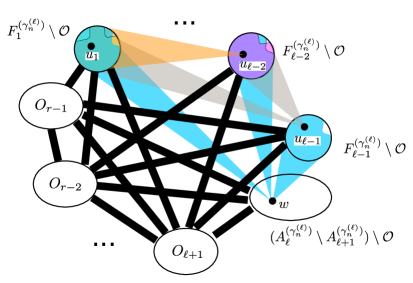
Figure 5.1. The black complete bipartite graphs are forced by Claim 5.15. The almost complete connections depicted with colours follow from the fact that the respective vertices lie in the sets $A_{j}^{\left(\gamma_{n}^{(\ell)}\right)}$ ($j=\ell,\ell-1,\ldots,2)$, and thus are well-connected to the sets $F_{t}^{\left(\gamma_{n}^{(\ell)}\right)}$ (for each $t\in[j-1]$).

We can refine this construction to find a positive $\nu^{r}$-measure of $K_{r}$-cliques as follows. First we take $w_{P}\in P$ and $w_{Q}\in Q$ such that $W(w_{P},w_{Q})>0$ (we have a $\nu^{2}$-positive measure of such choices). Then we sequentially find vertices

$$u_{\ell-1}\in F_{\ell-1}^{\left(\gamma_{n}^{(\ell)}\right)}\setminus\mathcal{O},\ldots,u_{1}\in F_{1}^{\left(\gamma_{n}^{(\ell)}\right)}\setminus\mathcal{O}$$

that are neighbors of $w_{P}$, $w_{Q}$ and the vertices fixed in the previous rounds. Having chosen the $K_{\ell+1}$-clique $w_{P}w_{Q}u_{\ell-1}u_{\ell-2}\ldots u_{1}$, Claim 5.8 tells us that $O_{\ell+1},O_{\ell+2},\ldots,O_{r-1}$ are disjoint, then together with Claim 5.15 we know that padding arbitrary elements from $O_{\ell+1},O_{\ell+2},\ldots,O_{r-1}$ yields a copy of $K_{r}$. Since all these sets have positive measure, we get a contradiction to (5.27). ∎

Proof of Claim 5.13.

Recall that $O_{\ell}$ arises from the weak* limit of the sets $A_{\ell}^{\left(\gamma_{n}^{(\ell)}\right)}\setminus A_{\ell+1}^{\left(\gamma_{n}^{(\ell)}\right)}$. Claims 5.8 and 5.9 tell us that $O_{\ell}$ can also be seen as the weak^∗ limit of the sets

$$\left(A_{\ell}^{\left(\gamma_{n}^{(\ell)}\right)}\setminus A_{\ell+1}^{\left(\gamma_{n}^{(\ell)}\right)}\right)\setminus\left(O_{\ell+1}\cup O_{\ell+2}\cup\ldots\cup O_{r-1}\cup\mathrm{supp\>}\mathfrak{c}\right)\;.$$

Thus the claim follows by combining Claim 5.12 and Lemma 2.4. ∎

Proof of Claim 5.14.

The fact that $\left(\chi_{\ell}\right)_{\Omega\setminus O_{\ell}}=0$ follows simply because $O_{\ell}$ is the indicator of $\mathrm{supp\>}\chi_{\ell}$. Suppose now for contradiction that $\left(\chi_{\ell}\right)_{O_{\ell}}$ is less than 1 on a set of positive measure. Combining this with (5.22) gives that $\nu(O_{\ell})>1-\delta$. This, however cannot be the case since $\delta(W)\geq\delta$ and $O_{\ell}$ is an independent set by Claim 5.13. ∎

Proof of Claim 5.15.

This follows by combining Claim 5.7, Claim 5.13, and the fact that the minimum degree of $W$ is at least $\delta$. ∎

6. Comparing the proofs

If not counting preparations related to the Regularity method, then the heart of Komlós’s proof of Theorem 1.2 in [10] is a less than three pages long calculation. In comparison, the corresponding part of our proof in Section 5.2 has circa four pages. So, our proof is not shorter, but it is conceptually much simpler. Indeed, Komlós’s proof proceeds by an ingenious iterative regularization of the host graph, a technique which was novel at that time and which is rare even today (apart from proofs of variants of Komlós’s Theorem, such as [19, 7]).

Our graphon formalism, on the other hand, allows us to proceed with the most pedestrian thinkable proof strategy. That is, to show using relatively straightforward calculations that no small fractional $H$-covers exist.

Let us note that our proof can be de-graphonized as follows. Consider a graph $G$ satisfying the minimum-degree condition as in (1.3). Apply the min-degree form of the Regularity lemma, thus arriving to a cluster graph $R$. Now, the calculations from Section 5.2 can be used mutatis mutandis to prove that $R$ contains no small fractional $H$-cover. Thus, by LP duality, the cluster graph $R$ contains a large fractional $H$-tiling. This fractional $H$-tiling in $R$ can be pulled back to a proportionally sized integral $H$-tiling in $G$ by Blow-up lemma type techniques. The advantage of this approach is that it allows the above mentioned argument “take a vertex which has the smallest value of $\mathfrak{c}$ and consider its neighborhood” (on the level of the cluster graph), but this is compensated by the usual technical difficulties like irregular or low density pairs.

7. Further possible applications

While Komlós’s Theorem provides a complete answer (at least asymptotically) for lower-bounding $\mathsf{til}(H,G)$ in terms of the minimum degree of $G$, the average degree version of the problem is much less understood. Apart from the Erdős–Gallai Theorem ($H=K_{2}$) mentioned in Section 1, the only other known graphs for which the asymptotic $F$-tiling thresholds have been determined are all bipartite graphs, [7] and $K_{3}$, [1]. The current graphon formalism may be of help in finding further density thresholds.

After this paper was made public, Piguet and Saumell [15, 14] used a similar approach (with the de-graphonized formalism, as described in Section 6) to obtain a strengthening of Komlós’s Theorem. In that strengthening, the lower-bound (1.3) is not required for all vertices but rather only for a certain (and optimal) proportion (which depends on $x$ and the graph $H$) of them.

Let us remark that in [4], the authors provide a graphon proof of the Erdős–Gallai Theorem. The key tool to this end is to establish the half-integrality property of the fractional vertex cover “polyton”. These objects are defined in analogy to fractional vertex cover potypes of graphs, but for graphons (hence the “-on” ending). This half-integrality property is a direct counterpart to the well-known statement about fractional vertex cover polytopes of finite graphs.

8. Acknowledgments

JH would like thank Dan Král and András Máthé for useful discussions that preceded this project. He would also like to thank Martin Doležal for the discussions they have had regarding functional analysis. We thank the referees for their helpful comments.

Part of this paper was written while JH was participating in the program Measured group theory at The Erwin Schrödinger International Institute for Mathematics and Physics.

The contents of this publication reflects only the authors’ views and not necessarily the views of the European Commission of the European Union. This publication reflects only its authors’ view; the European Research Council Executive Agency is not responsible for any use that may be made of the information it contains.

References

- [1] P. Allen, J. Böttcher, J. Hladký, and D. Piguet. A density Corrádi-Hajnal theorem. Canad. J. Math., 67(4):721–758, 2015.
- [2] C. Borgs, J. T. Chayes, L. Lovász, V. T. Sós, and K. Vesztergombi. Convergent sequences of dense graphs. I. Subgraph frequencies, metric properties and testing. Adv. Math., 219(6):1801–1851, 2008.
- [3] A. Bruckner, J. Bruckner, and B. Thomson. Real Analysis. ClassicalRealAnalysis.com, second edition, 2008.
- [4] M. Doležal and J. Hladký. Matching polytons. arXiv:1606.06958.
- [5] P. Erdős and T. Gallai. On maximal paths and circuits of graphs. Acta Math. Acad. Sci. Hungar, 10:337–356 (unbound insert), 1959.
- [6] P. Erdős and A. H. Stone. On the structure of linear graphs. Bulletin of the American Mathematical Society, 52:1087–1091, 1946.
- [7] C. Grosu and J. Hladký. The extremal function for partial bipartite tilings. European J. Combin., 33(5):807–815, 2012.
- [8] A. Hajnal and E. Szemerédi. Proof of a conjecture of P. Erdős. In Combinatorial theory and its applications, II (Proc. Colloq., Balatonfüred, 1969), pages 601–623. North-Holland, Amsterdam, 1970.
- [9] J. Hladký, P. Hu, and D. Piguet. Tilings in graphons. arXiv:1606.03113.
- [10] J. Komlós. Tiling Turán theorems. Combinatorica, 20(2):203–218, 2000.
- [11] D. Kühn and D. Osthus. The minimum degree threshold for perfect graph packings. Combinatorica, 29(1):65–107, 2009.
- [12] L. Lovász. Large networks and graph limits, volume 60 of American Mathematical Society Colloquium Publications. American Mathematical Society, Providence, RI, 2012.
- [13] L. Lovász and B. Szegedy. Limits of dense graph sequences. J. Combin. Theory Ser. B, 96(6):933–957, 2006.
- [14] D. Piguet and M. Saumell. A median-type condition for graph tiling.
- [15] D. Piguet and M. Saumell. A median-type condition for graph tiling. In European Conference on Combinatorics, Graph Theory and Applications (EuroComb 2017), volume 61 of Electron. Notes Discrete Math., pages 979–985. Elsevier Sci. B. V., Amsterdam, 2017.
- [16] A. A. Razborov. Flag algebras. J. Symbolic Logic, 72(4):1239–1282, 2007.
- [17] M. Simonovits. A method for solving extremal problems in graph theory, stability problems. In Theory of Graphs (Proc. Colloq., Tihany, 1966), pages 279–319. Academic Press, New York, 1968.
- [18] T. Tao. An epsilon of room, I: real analysis, volume 117 of Graduate Studies in Mathematics. American Mathematical Society, Providence, RI, 2010. Pages from year three of a mathematical blog.
- [19] A. Treglown. A degree sequence Hajnal–Szemerédi theorem. J. Combin. Theory Ser. B, 118:13–43, 2016.