Analysis of DIS structure functions of the nucleon within truncated Mellin moments approach[$\star$]t1

Abstract

We present generalized evolution equations and factorization in terms of the truncated Mellin moments (TMM) of the parton distributions and structure functions. We illustrate the $x$ and $Q^{2}$ dependence of TMM in the polarized case. Using the TMM approach we compare the integrals of $g_{1}$ with HERMES and COMPASS data from the limited $x$-ranges.

1 Introduction

Our knowledge of the matter structure and fundamental particle interactions in high energy regimes is mostly provided by deep inelastic scattering (DIS) of leptons on hadrons and hadron-hadron collisions. According to the factorization theorem (for a review see, for instance, Collins:1989gx ), the cross sections for DIS and hadron - hadron collisions can be represented as convolution of short-distance perturbative and long-distance nonperturbative parts. The perturbative part describing partonic cross sections at a sufficiently high scale of the momentum transfer $Q$ is calculable within the perturbative QCD. In turn, the non-perturbative part contains universal process independent parton distribution functions (PDFs) and fragmentation functions (FFs), which can be obtained from experimental data. The evolution of PDFs and FFs with the interaction scale $Q^{2}$ is again described with the use of the perturbative QCD methods. Usually, one uses the standard DGLAP approach Gribov:1972ri , Gribov:1972rt , Dokshitzer:1977sg , Altarelli:1977zs to calculate parton densities at a given scale $Q^{2}$ when these densities are assumed for a certain input scale $Q_{0}^{2}$. Traditionally, in the QCD description of the nucleon structure, the central role is played by the quark and gluon distribution functions and their evolution equations. Then, Mellin moments of the parton distributions and structure functions (SFs), which are essential in testing sum rules, are obtained as integrals of the distribution or structure functions over the Bjorken-$x$ variable. An alternative approach, in which one can study directly the evolution of the truncated moments of the parton distributions was proposed in Forte:1998nw , Forte:2000wh , Piccione:2001vf , Forte:2002us . Later on, we elaborated the exact evolution equations for the truncated moments of the parton densities and structure functions Kotlorz:2006dj , Kotlorz:2011pk , Kotlorz:2014kfa . We found that the $n$th truncated Mellin moment obeys the DGLAP evolution but with the transformed kernel $P(x)^{\prime}=P(x)x^{n}$. Also, the coefficient functions for the truncated moments of the structure functions have a simple rescaled form $C(x)^{\prime}=x^{n}C(x)$. In fact, the TMM approach is a generalization of the well-known DGLAP evolution for PDFs, where one obtains the answer for the generalized TMM which can be one of the many possible constructions, e.g.: PDFs $f(x,Q^{2})$, SFs $F(x,Q^{2}$ themselves, their truncated or untruncated $n$th moments, multi-integrations or multi-differentiations of $f$ Kotlorz:2014fia . The major advantage of the TMM approach is a possibility to adapt theoretical analysis of the nucleon structure functions to the experimentally accessible region as the measurements do not extend to a very large and a very small Bjorken-$x$ variable. Furthermore, solving the evolution equations for truncated moments, one does not need to assume exact forms of the input parametrizations of the parton densities, which like, e.g., polarized gluon distributions, are weakly known. The extraction of the truncated moments of PDFs or SFs from the data carries smaller uncertainties than the extraction of PDFs or SFs themselves. The TMM of the original function $f$ for $n\geq 1$ are less singular in $x$ than $f$ itself and all of the DGLAP evolution and convolution Wilson kernels, which simply rescale to $x^{n}P(x)$, $x^{n}C(x)$, are also less singular than $P$ and $C$, respectively. Hence, numerical analysis based directly on the evolution of truncated moments is faster, more stable and accurate in comparison with the traditional approach based on PDFs. These advantages make the TMM approach a promising tool in QCD studies, providing direct methods to test different unpolarized and polarized sum rules in each order of perturbation expansion. This is crucial for instance, in finding out how the nucleon spin is distributed among its constituents: quarks and gluons. A number of important problems in particle physics, e.g., solving of the mentioned above ‘nucleon spin puzzle’, quark - hadron duality or higher twist contributions to the structure functions refers directly to moments. These issues initiate a large number of experimental and theoretical studies as well. The TMM approach can be very helpful in these projects.

The aim of this paper is to acquaint the Reader with the TMM approach and encourage Her/Him to take it into account in Her/His own studies. The content of this paper is as follows. In the next section, we present the main results of the TMM approach for PDFs and SFs. In Sec. 3, we illustrate the $Q^{2}$ evolution of the polarized PDFs and SFs in terms of the TMM. We also compare the predictions for contributions to the first moment of the structure function $g_{1}$ with HERMES and COMPASS data from the limited $x$-ranges.

2 Generalized evolution for TMM of the parton distributions and structure functions

As it has already been mentioned in the Introduction, the truncated moments of the original function $f$ in their general form may assume many different constructions, useful in analysis of the nucleon structure functions. Each of these TMM obeys the DGLAP evolution with a very simply rescaled kernel $P_{ij}(x)$. The Reader can find the summarized results in the Appendix A and more details on this subject in Kotlorz:2014fia , Strozik-Kotlorz:2015gka , Strozik-Kotlorz:2015iqr . We also proposed there the generalized Bjorken sum rule as an example of application of the TMM. Here, in this paper we shall focus on the original version of the evolution equations for the TMM Kotlorz:2006dj . We shall present the suitable evolution equations and relations for the TMM of the parton distribution functions in Sec. 2.1 and structure functions in Sec. 2.2.

2.1 Evolution of the PDFs and their TMM

In the TMM approach to the DGLAP evolution the main role is played by the truncated integrals of the original functions $f(x)$,

$$f^{n}(x)\equiv\int\limits_{x}^{1}dz\,z^{n-1}\,f(z),$$ (1)

where $f(x)$ can be any unpolarized $q$ or polarized $\Delta q$ parton distribution function and $f^{n}(x)$ defines its $n$th moment truncated at $x$.

Throughout this paper, we use the following notation: $q(x,Q^{2})$, $\bar{q}(x,Q^{2})$, $G(x,Q^{2})$, $\Delta q(x,Q^{2})$, $\Delta\bar{q}(x,Q^{2})$, $\Delta G(x,Q^{2})$ denote PDFs, while $q^{n}(x,Q^{2})$, $\bar{q}^{n}(x,Q^{2})$, $G^{n}(x,Q^{2})$, $\Delta q^{n}(x,Q^{2})$, $\Delta\bar{q}^{n}(x,Q^{2})$, $\Delta G^{n}(x,Q^{2})$ are their TMM, defined as in Eq. (1), respectively.

The well-known DGLAP evolution equations for the nonsinglet distributions $q_{NS}$ take the form

$$\frac{\partial}{\partial\ln Q^{2}}q_{NS}(x,Q^{2})=\frac{\alpha_{s}(Q^{2})}{2\pi}\;(P_{qq}\ast q_{NS})(x,Q^{2})$$ (2)

and for the singlet $q_{S}$ and gluon distributions $G$ they are the matrix equation,

$$\frac{\partial}{\partial\ln Q^{2}}\begin{pmatrix}q_{S}(x,Q^{2})\\ G(x,Q^{2})\end{pmatrix}=$$

$$\frac{\alpha_{s}(Q^{2})}{2\pi}\left(\begin{pmatrix}P_{qq}&P_{qG}\\ P_{Gq}&P_{GG}\end{pmatrix}\ast\begin{pmatrix}q_{S}\\ G\end{pmatrix}\right)(x,Q^{2}).$$ (3)

In the above equations, $\ast$ denotes the Mellin convolution,

$$(P\ast q)(x,Q^{2})\equiv\int\limits_{x}^{1}\frac{dz}{z}\;P\left(\frac{x}{z}\right)q(z,Q^{2}).$$ (4)

Each splitting function $P_{ij}$ is calculable as a power series in the strong coupling constant $\alpha_{s}$,

$$P_{ij}(x,\alpha_{s})=\left[\,P_{ij}^{(0)}(x)+\frac{\alpha_{s}(Q^{2})}{2\pi}P_{ij}^{(1)}(x)+\cdots\,\right].$$ (5)

For the polarized parton densities $\Delta q_{i}(x,Q^{2})$, $\Delta G(x,Q^{2})$ the evolution equations have the same form, Eqs. (2), (2.1), but with the polarized splitting functions $\Delta P_{ij}(x,\alpha_{s})$, respectively.

Taking into account the properties of the Mellin convolution and the basic physical condition that parton densities disappear for $x>1$, we found in Kotlorz:2006dj that the truncated moments of the parton distributions defined in Eq. (1) also obey the DGLAP evolution equations with slightly modified evolution kernels, namely

$$\frac{\partial}{\partial\ln Q^{2}}q^{n}_{NS}(x,Q^{2})=\frac{\alpha_{s}(Q^{2})}{2\pi}\;(P^{\prime}_{qq}\ast q^{n}_{NS})(x,Q^{2}),$$ (6)

$$\frac{\partial}{\partial\ln Q^{2}}\begin{pmatrix}q^{n}_{S}(x,Q^{2})\\ G^{n}(x,Q^{2})\end{pmatrix}=$$

$$\frac{\alpha_{s}(Q^{2})}{2\pi}\left(\begin{pmatrix}P^{\prime}_{qq}&P^{\prime}_{qG}\\ P^{\prime}_{Gq}&P^{\prime}_{GG}\end{pmatrix}\ast\begin{pmatrix}q^{n}_{S}\\ G^{n}\end{pmatrix}\right)(x,Q^{2}),$$ (7)

where

$$P^{\prime}_{ij}(x,\alpha_{s})=x^{n}P_{ij}(x,\alpha_{s}).$$ (8)

Similar equations hold in the polarized case:

$$\frac{\partial}{\partial\ln Q^{2}}\Delta q^{n}_{NS}(x,Q^{2})=\frac{\alpha_{s}(Q^{2})}{2\pi}\;(\Delta P^{\prime}_{qq}\ast\Delta q^{n}_{NS})(x,Q^{2}),$$ (9)

$$\frac{\partial}{\partial\ln Q^{2}}\begin{pmatrix}\Delta q^{n}_{S}(x,Q^{2})\\ \Delta G^{n}(x,Q^{2})\end{pmatrix}=$$

$$\frac{\alpha_{s}(Q^{2})}{2\pi}\left(\begin{pmatrix}\Delta P^{\prime}_{qq}&\Delta P^{\prime}_{qG}\\ \Delta P^{\prime}_{Gq}&\Delta P^{\prime}_{GG}\end{pmatrix}\ast\begin{pmatrix}\Delta q^{n}_{S}\\ \Delta G^{n}\end{pmatrix}\right)(x,Q^{2}),$$ (10)

where again as in Eq. (8)

$$\Delta P^{\prime}_{ij}(x,\alpha_{s})=x^{n}\Delta P_{ij}(x,\alpha_{s}).$$ (11)

Since existing measurements cover only a restricted range in $x$, $x_{min}\leq x\leq x_{max}$, it is useful to consider the double truncated Mellin moments of PDFs which are defined by:

$$f^{n}(x_{1},x_{2})=\int\limits_{x_{1}}^{x_{2}}dx\;x^{n-1}\,f(x).$$ (12)

It is straightforward to show that the double truncated moments, Eq. (12), being a subtraction of two single truncated ones,

$$f^{n}(x_{1},x_{2})=f^{n}(x_{1})-f^{n}(x_{2}),$$ (13)

also fulfill the analogical DGLAP equations Psaker:2008ju , Kotlorz:2011pk :

$$\frac{\partial}{\partial t}q^{n}_{NS}(x_{1},x_{2},Q^{2})=$$

$$\frac{\alpha_{s}(Q^{2})}{2\pi}\;\int\limits_{x_{1}}^{1}\frac{dz}{z}\;P^{\prime}(z)\;q^{n}_{NS}\left(\frac{x_{1}}{z},\frac{x_{2}}{z},Q^{2}\right).$$ (14)

Notice that the evolution equations for the double truncated moments Eq. (2.1) are in fact a generalization of those for the single truncated and untruncated ones. Setting $x_{2}=1$ one obtains Eq. (6), while setting $x_{1}=0$ and $x_{2}=1$ one obtains the well-known renormalization group equations for the untruncated moments:

$$\frac{\partial}{\partial\ln Q^{2}}q^{n}_{NS}(Q^{2})=\frac{\alpha_{s}(Q^{2})}{2\pi}\,\gamma^{n}_{qq}(Q^{2})q^{n}_{NS}(Q^{2}).$$ (15)

2.2 Evolution of SFs and their TMM

Similarly to the evolution of the TMM of PDFs, where the splitting functions have a simply modified form, Eq. (8), the coefficient functions of the $n$th truncated moments for structure functions are changed in the same manner Kotlorz:2014kfa . Namely, if $F$ denotes SF

$$F(x)=(C*f)(x),$$ (16)

then the TMM of $F$,

$$F^{n}(x)\equiv\int\limits_{x}^{1}z^{n-1}F(z)\,dz$$ (17)

takes the form

$$F^{n}(x)=(C^{\prime}*f^{n})(x),$$ (18)

where $f^{n}$ is the TMM of PDF $f$ defined in Eq. (1) and $C^{\prime}$ is the new coefficient function

$$C^{\prime}(x)=x^{n}C(x).$$ (19)

Let us demonstrate this for a case of the polarized structure function $g_{1}$.

In the NLO approximation within the ${\bar{M}S}$ scheme $g_{1}(x,Q^{2})$ is given by

$$g_{1}(x,Q^{2}) = \frac{1}{2}\sum_{q}e_{q}^{2}\Big{[}\Delta q(x,Q^{2})+\Delta\bar{q}(x,Q^{2})$$ (20)

$$+ \frac{\alpha_{s}(Q^{2})}{2\pi}\Big{(}(\Delta C_{q}*(\Delta q+\Delta\bar{q}))(x,Q^{2})$$

$$+ (2\Delta C_{G}*\Delta G)(x,Q^{2})\Big{)}\Big{]},$$

where $\Delta C_{i}$ denotes the spin dependent coefficient functions and $\Delta\bar{q}$ is the antiquark polarized PDF. According to Eqs. (16)–(19), the $n$th TMM of $g_{1}$,

$$g_{1}^{n}(x,Q^{2})=\int\limits_{x}^{1}z^{n-1}g_{1}(z,Q^{2})\,dz$$ (21)

obtains the following form:

$$g_{1}^{n}(x,Q^{2}) = \frac{1}{2}\sum_{q}e_{q}^{2}\Big{[}\Delta q^{n}(x,Q^{2})+\Delta\bar{q}^{n}(x,Q^{2})$$ (22)

$$+ \frac{\alpha_{s}(Q^{2})}{2\pi}\Big{(}(\Delta C^{\prime}_{q}*(\Delta q^{n}+\Delta\bar{q}^{n}))(x,Q^{2})$$

$$+ (2\Delta C^{\prime}_{G}*\Delta G^{n})(x,Q^{2})\Big{)}\Big{]}$$

where

$$\Delta C^{\prime}_{q,G}(x)=x^{n}\Delta C_{q,G}(x).$$ (23)

Finally, we also would like to mention some results for the function $g_{2}$, implied by the TMM approach.

In Kotlorz:2011pk , we derived the Wandzura-Wilczek (WW) relation Wandzura:1977qf for the TMM, and found partial contributions to the Burkhardt-Cottingham (BC) Burkhardt:1970ti sum rule. Namely, the WW relation in terms of the TMM reads

$$g_{2}^{n}(x,Q^{2})=\frac{1-n}{n}\>g_{1}^{n}(x,Q^{2})-\frac{x^{n}}{n}\>g_{1}^{0}(x,Q^{2}),$$ (24)

where

$$g_{1,2}^{n}(x,Q^{2})=\int\limits_{x}^{1}dz\,z^{n-1}\,g_{1,2}(z,Q^{2}).$$ (25)

In a case of the first moment ($n=1$), from Eq. (24) one gets

$$\int\limits_{x_{1}}^{x_{2}}dx\,g_{2}^{WW}(x,Q^{2})=$$

$$-x_{1}\int\limits_{x_{1}}^{x_{2}}\frac{dz}{z}\,g_{1}(z,Q^{2})+(x_{2}-x_{1})\int\limits_{x_{2}}^{1}\frac{dz}{z}\,g_{1}(z,Q^{2}).$$ (26)

The above equations can be used to testing the BC sum rule and other TMM of $g_{2}$.

The advantage of the TMM approach is the possibility to have a convenient procedure that combines direct evolution of important physical quantities with factorization in a smaller number of steps than the widely-known approach based on PDFs. Furthermore, since the suitable functions in the TMM approach are mostly more regular (less singular for very small $x$) than in the case of PDFs, the numerical procedures used in the TMM approach are more stable than those for the standard PDFs approach.

3 TMM results for the spin PDFs and SFs

One of the most important goals in the recent studies of QCD is understanding of the nucleon spin structure and determination of the individual partonic contributions to the helicity of the nucleon,

$$\Delta q(Q^{2})=\int\limits_{0}^{1}dx\,\Delta q(x,Q^{2}).$$ (27)

Measurements of the spin structure functions $g_{1}$ and $g_{2}$, which parametrize the cross section of polarized inclusive DIS, are always performed in the restricted $x$-range. This limitation provides results, which are the partial (truncated) moments of the parton helicity distributions,

$$\Delta q(x_{1},x_{2},Q^{2})=\int\limits_{x_{1}}^{x_{2}}dx\,\Delta q(x,Q^{2}),$$ (28)

instead of the full moments, Eq. (27). Thus, the TMM, and especially the first TMM of the polarized PDFs and SFs, are quantities of large importance. The approach, presented here, allows one a direct study of these quantities.

Here we present the numerical results for evolution of the TMM. In Figs. 1–10, we illustrate the $x$ and $Q^{2}$ dependence of the TMM of the polarized PDFs and SFs in LO and NLO. We solve the evolution Eqs. (9)–(11) in the $x$-space and also use the factorization formula for SF $g_{1}$, Eqs. (22)–(23) (for more details, see Appendix B). Finally, in Table 1, we present a comparison with HERMES Airapetian:2006vy and COMPASS Adolph:2015saz data on the first TMM of the spin SF $g_{1}$. We show results for the partial contributions to the integrals of $g_{1}$,

$$\Gamma_{1}(x_{1},x_{2},Q^{2})=\int\limits_{x_{1}}^{x_{2}}dx\,g_{1}(x,Q^{2}),$$ (29)

for the proton, neutron, deuteron, nucleon and the nonsinglet part. The truncated contribution to the nonsinglet SF,

$$\int\limits_{x_{1}}^{x_{2}}dx\,g_{1,NS}(x,Q^{2})=\int\limits_{x_{1}}^{x_{2}}dx\,(g_{1,p}-g_{1,n})(x,Q^{2})$$ (30)

is crucial in determination of the Bjorken Sum Rule (BSR) Bjorken:1966jh , Bjorken:1969mm .

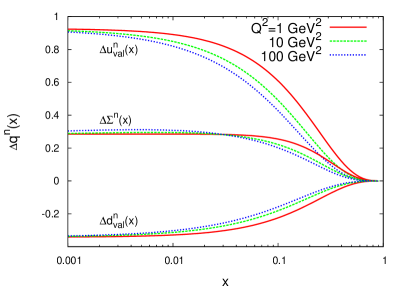
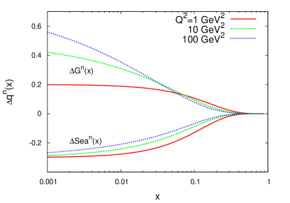
Figure 1: The first TMM ($n=1$) of the polarized PDFs, $\int\limits_{x}^{1}dz\,\Delta q(z,Q^{2})$, as a function of the low-$x$ limit of integration, at different $Q^{2}$, in NLO.

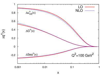
Figure 2: A comparison of LO and NLO evolution of the first TMM of $\Delta u_{val}$, $\Delta Sea$, $\Delta G$, vs the low-$x$ limit of integration, at $Q^{2}=100\;\rm{GeV}^{2}$.

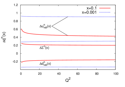
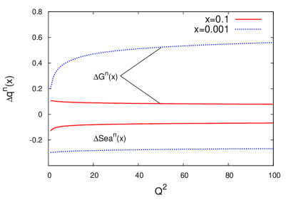
Figure 3: The first TMM of the polarized PDFs, as a function of $Q^{2}$, for two low-$x$ limits of integration, in NLO.

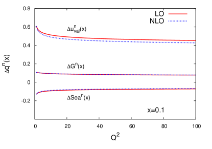
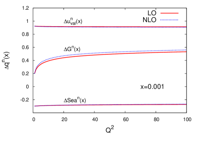
Figure 4: A comparison of LO and NLO evolution of the first TMM of $\Delta u_{val}$, $\Delta Sea$ and $\Delta G$, vs $Q^{2}$, at two low-$x$ limits of integration.

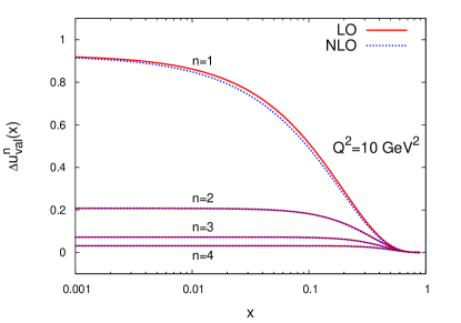
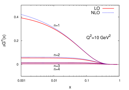
Figure 5: A comparison of LO and NLO evolution of four TMMs ($n=1,\,2,\,3,\,4$) of $\Delta u_{val}$ and $\Delta G$, vs low-$x$ limit of integration, at $Q^{2}=10\;\rm{GeV}^{2}$.

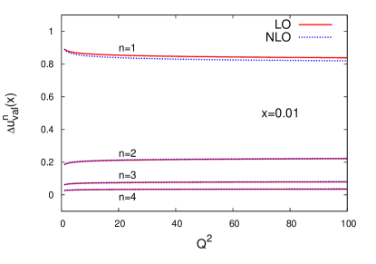
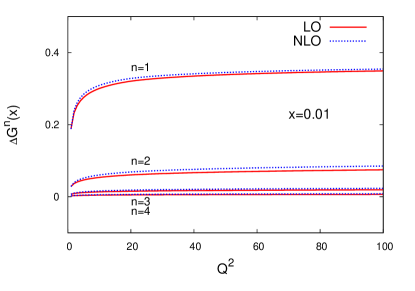
Figure 6: A comparison of LO and NLO evolution of four TMMs ($n=1,\,2,\,3,\,4$) of $\Delta u_{val}$ and $\Delta G$, vs $Q^{2}$, at low-$x$ limit of integration 0.01.

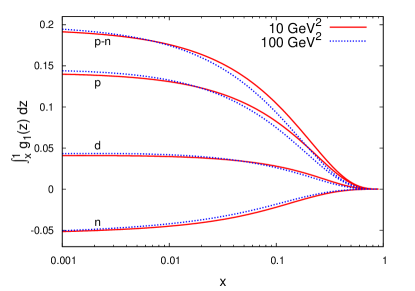
Figure 7: The first TMM of the polarized SF $g_{1}$, for the proton ($p$), deuteron ($d$), neutron ($n$) and the nonsinglet part ($NS=p-n$), $\int\limits_{x}^{1}dz\,g_{1}(z,Q^{2})$, as a function of the low-$x$ limit of integration, for two values of $Q^{2}$, in NLO.

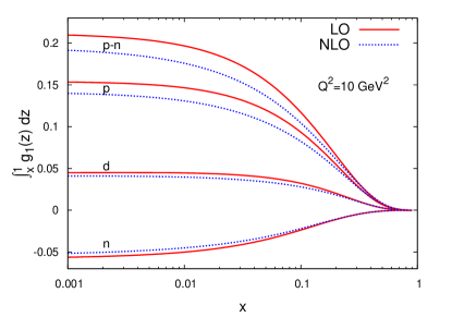
Figure 8: A comparison of LO and NLO evolution of the first TMM of $g_{1}$, for the proton, deuteron, neutron and the nonsinglet part, as a function of the low-$x$ limit of integration, at $Q^{2}=10\;\rm{GeV}^{2}$.

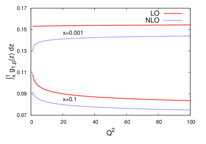
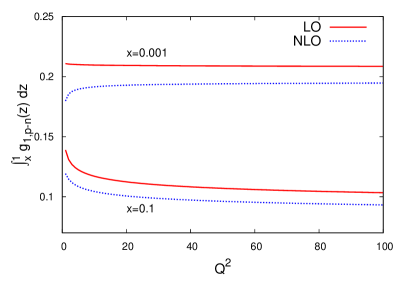
Figure 9: A comparison of LO and NLO evolution of the first TMM of $g_{1}$, for the proton and the nonsinglet part (p-n), vs $Q^{2}$, for two low-$x$ limits of integration.

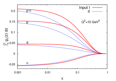
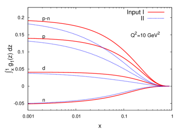
Figure 10: A comparison of the impact of the different small-$x$ behaviour of the polarized nonsinglet PDFs on the LO (left) and NLO (right) evolution of the first TMM of $g_{1}$. The details on Input I and Input II are given in Appendix B.

Table 1: First TMM of $g_{1}$ in NLO. Comparison with HERMES Airapetian:2006vy and COMPASS Adolph:2015saz data. $g_{1,N}=\frac{1}{2}(g_{1,p}+g_{1,n})$.

Experiment	Type	Exp. value	Input I	Input II
HERMES	proton	$0.1211\pm 0.0025\pm 0.0068$	0.1220	0.09513
$Q^{2}=5\;\rm{GeV}^{2}$	deuteron	$0.0436\pm 0.0012\pm 0.0018$	0.03724	0.02651
$x$-range: 0.021 – 0.9	p-n	$0.1479\pm 0.0055\pm 0.0142$	0.1635	0.1329
COMPASS	proton	$0.134\pm 0.003$	0.1334	0.1229
$Q^{2}=3\;\rm{GeV}^{2}$	N	$0.047\pm 0.003$	0.04186	0.03737
$x$-range: 0.0025 – 0.7	p-n	$0.170\pm 0.008$	0.1832	0.1710

4 Summary

Our goal in this paper was to present the TMM approach as a convenient tool in QCD analysis that combines direct evolution of important physical quantities with factorization in a smaller number of steps than the standard approach based on PDFs. Splitting functions $P^{\prime}$ and coefficient functions $C^{\prime}$ for the TMM have simple forms $P^{\prime}=x^{n}P$ and $C^{\prime}=x^{n}C$, which enables one to use the standard methods of solving the DGLAP equations only with tiny modifications. From the technical point of view, the TMM less suffer from experimental uncertainties, and also the numerical procedures involved into the TMM approach are more stable than those for PDFs. The TMM approach is, on the one hand, a generalization of the DGLAP evolution and, on the other hand, allows a better fit of the theoretical methods to the limitations of experimental measurements on the kinematic variables $x$ and $Q^{2}$. The perturbative QCD itself explores truncated evolution in $Q^{2}>\mu^{2}$; also the Bjorken variable $x\rightarrow 0$ has no physical meaning (it means infinite energy). Hence, the use of the methods, which incorporate these limitations in a natural way is very advantageous.

Appendix A Generalized evolution DGLAP

The TMM of the parton densities, Eq. (1), and also the generalized truncated moments obtained by multiple integrations as well as multiple differentiations of the original parton distribution satisfy the DGLAP equations with the simply transformed evolution kernel Kotlorz:2006dj , Kotlorz:2011pk , Kotlorz:2014kfa , Kotlorz:2014fia . In Table 2, we summarize the generalized TMM together with the correspondingly transformed DGLAP evolution kernels.

Table 2: TMM and the corresponding evolution kernels

Description	Generalized form	DGLAP evolution kernel ${\cal P}$
Original PDF	$f(x)$	$P(y)$
$n$th TMM of PDF	$\int\limits_{z}^{1}x^{n-1}\,f(x)\,dx$	$P(y)\cdot y^{n}$
Multiple integration	$\int\limits_{z}^{1}z_{k}^{n_{k}-1}dz_{k}\>...\int\limits_{z_{2}}^{1}z_{1}^{n_{1}-1}\;f(z_{1})\;dz_{1}$	$P(y)\cdot y^{n_{1}+n_{2}+...+n_{k}}$
Multiple differentiation	$\left(-\frac{d}{dx}\right)^{k}\left[x^{n}f(x)\right]$	$P(y)\cdot y^{n-k}$
Convolution with
normalized function $\omega(x)$,	$\omega\ast fx^{n}\equiv\int\limits_{z}^{1}x^{n-1}\,\omega\left(z/x\right)\,f(x)\,dx$	$P(y)\cdot y^{n}$
$\int\limits_{0}^{1}\omega(t)\,dt=1$

Appendix B The direct solving of the evolution equations for TMM

For a fixed $n$, the truncated moment of $f$ Eq. (1) is, like the $f$ itself, a function of two variables: $x$ - the lower limit of the integration and $Q^{2}$. The similarity of the evolution equations for the TMM, Eqs. (6)–(8), to the ordinary DGLAP for PDFs, Eqs. (2)–(4), enables one to use the same methods of solving in both the cases. In literature, there are two basic methods of solving the DGLAP evolution equations for the function $f$: in the $x$ space with the help of the polynomial expansions of $f$, (see e.g. Kumano:2004dw ), or in the moment space. The use of the moment space gives the possibility to get analytical solutions for the moments and then, the function $f$ can be obtained via the inverse Mellin transform. Solving the evolution equation for the TMM in the $n$ space, one encounters the objects ‘moment of moment’ and the problem how to deal with them. In Kotlorz:2011pk , we derived for this aim useful relations between untruncated and truncated Mellin moments.

In many our previous TMM analyses we used the Chebyshev polynomials expansion which is one of the methods of solving the DGLAP equations in the $x$ space, reducing the former differentio-integral equations to a system of linear differential ones El-gendi:1969 . In this work, for carrying out the DGLAP evolution for the TMM in the $x$-space we adapted the Hoppet package Salam:2008qg , which we appropriately changed. As an example, we solve the polarized case of evolution, Eqs. (9)–(11), with input truncated moments at $Q_{0}^{2}=1\rm{GeV}^{2}$,

$$\Delta q^{n}(x,Q_{0}^{2})\equiv\int\limits_{x}^{1}dz\,z^{n-1}\,\Delta q(z,Q_{0}^{2}).$$ (31)

We assume distributions $\Delta q(z,Q_{0}^{2})$ in the form

$$\Delta q_{i}(x,Q_{0}^{2})=\frac{N_{i}x^{a_{i}}(1-x)^{b_{i}}}{\int\limits_{0}^{1}x^{a_{i}}(1-x)^{b_{i}}\,dx}\,,$$ (32)

where $a_{\bar{s}}=a_{G}=0$, $b_{uval}=b_{dval}=3$, $b_{\bar{s}}=7$, $b_{G}=5$. In Input I, we also assume $a_{uval}=a_{dval}=0$, while in Input II, $a_{uval}=a_{dval}=-0.4$, that results from theoretical studies on the small-$x$ behaviour of the nonsinglet polarized PDFs Kwiecinski:1995rm , Bartels:1995iu . The normalization factors $N_{i}$ reflect the experimental data on the proton spin contributions: $N_{uval}+N_{dval}=0.585$, $N_{uval}-N_{dval}=1.270$, $2N_{\bar{s}}=-0.10$, $N_{G}=0.2$.

Instead of the the functional form of input PDFs in order to create the initial TMM, Eq. (31), one can represent directly the TMM on a $x$-space grid.

References

- (1) J.C. Collins, D.E. Soper, G.F. Sterman, Adv. Ser. Direct. High Energy Phys. 5, 1 (1989). DOI 10.1142/9789814503266-0001
- (2) V.N. Gribov, L.N. Lipatov, Sov. J. Nucl. Phys. 15, 438 (1972). [Yad. Fiz.15,781(1972)]
- (3) V.N. Gribov, L.N. Lipatov, Sov. J. Nucl. Phys. 15, 675 (1972). [Yad. Fiz.15,1218(1972)]
- (4) Y.L. Dokshitzer, Sov. Phys. JETP 46, 641 (1977). [Zh. Eksp. Teor. Fiz.73,1216(1977)]
- (5) G. Altarelli, G. Parisi, Nucl. Phys. B126, 298 (1977). DOI 10.1016/0550-3213(77)90384-4
- (6) S. Forte, L. Magnea, Phys. Lett. B448, 295 (1999). DOI 10.1016/S0370-2693(99)00065-9
- (7) S. Forte, L. Magnea, A. Piccione, G. Ridolfi, Nucl. Phys. B594, 46 (2001). DOI 10.1016/S0550-3213(00)00670-2
- (8) A. Piccione, Phys. Lett. B518, 207 (2001). DOI 10.1016/S0370-2693(01)01059-0
- (9) S. Forte, J.I. Latorre, L. Magnea, A. Piccione, Nucl. Phys. B643, 477 (2002). DOI 10.1016/S0550-3213(02)00688-0
- (10) D. Kotlorz, A. Kotlorz, Phys. Lett. B644, 284 (2007). DOI 10.1016/j.physletb.2006.11.054
- (11) D. Kotlorz, A. Kotlorz, Acta Phys. Polon. B42, 1231 (2011). DOI 10.5506/APhysPolB.42.1231
- (12) D. Kotlorz, A. Kotlorz, Phys. Part. Nucl. Lett. 11, 357 (2014). DOI 10.1134/S1547477114040153
- (13) D. Kotlorz, S.V. Mikhailov, JHEP 06, 065 (2014). DOI 10.1007/JHEP06(2014)065
- (14) D. Strozik-Kotlorz, S.V. Mikhailov, O.V. Teryaev, PoS BaldinISHEPPXXII, 033 (2015)
- (15) D. Strozik-Kotlorz, S.V. Mikhailov, O.V. Teryaev, J. Phys. Conf. Ser. 678(1), 012017 (2016). DOI 10.1088/1742-6596/678/1/012017
- (16) A. Psaker, W. Melnitchouk, M.E. Christy, C. Keppel, Phys. Rev. C78, 025206 (2008). DOI 10.1103/PhysRevC.78.025206
- (17) S. Wandzura, F. Wilczek, Phys. Lett. B72, 195 (1977). DOI 10.1016/0370-2693(77)90700-6
- (18) H. Burkhardt, W.N. Cottingham, Annals Phys. 56, 453 (1970). DOI 10.1016/0003-4916(70)90025-4
- (19) A. Airapetian, et al., Phys. Rev. D75, 012007 (2007). DOI 10.1103/PhysRevD.75.012007
- (20) C. Adolph, et al., Phys. Lett. B753, 18 (2016). DOI 10.1016/j.physletb.2015.11.064
- (21) J.D. Bjorken, Phys. Rev. 148, 1467 (1966). DOI 10.1103/PhysRev.148.1467
- (22) J.D. Bjorken, Phys. Rev. D1, 1376 (1970). DOI 10.1103/PhysRevD.1.1376
- (23) S. Kumano, T.H. Nagai, J. Comput. Phys. 201, 651 (2004). DOI 10.1016/j.jcp.2004.05.021
- (24) S.E. El-gendi, Comput. J. 12, 282 (1969). DOI 10.1093/comjnl/12.3.282
- (25) G.P. Salam, J. Rojo, Comput. Phys. Commun. 180, 120 (2009). DOI 10.1016/j.cpc.2008.08.010
- (26) J. Kwiecinski, Acta Phys. Polon. B27, 893 (1996)
- (27) J. Bartels, B.I. Ermolaev, M.G. Ryskin, Z. Phys. C70, 273 (1996)